Exact results for a toy model exhibiting dynamic criticality

Abstract

In this article we discuss an exactly solvable, one-dimensional, periodic toy charge density wave model introduced in [D.C. Kaspar, M. Mungan, EPL 103, 46002 (2013)]. In particular, driving the system with a uniform force, we show that the depinning threshold configuration is an explicit function of the underlying disorder, as is the evolution from the negative threshold to the positive threshold, the latter admitting a description in terms of record sequences. This evolution is described by an avalanche algorithm, which identifies a sequence of static configurations that are stable at successively stronger forcing, and is useful both for analysis and simulation. We focus in particular on the behavior of the polarization $P$, which is related to the cumulative avalanche size, as a function of the threshold force minus the current force $(F_{\mathrm{th}}-F)$, as this has been the focus of several prior numerical and analytical studies of CDW systems. The results presented are rigorous, with exceptions explicitly indicated, and show that the depinning transition in this model is indeed a dynamic critical phenomenon.

1 Introduction

We consider an infinite chain of particles connected by springs, where each particle is exposed to an external potential. The potentials are identical except for quenched random phase shifts. Such systems originally served as phenomenological models for charge density waves, a quantum phenomenon observed in certain materials at low temperature [1], but are now considered model problems in the study of the behavior of elastic manifolds in disordered media; see [2, 3, 4] for reviews.

Under the influence of an external driving force, the particles move, perhaps within a single well of the substrate, or from one well to another. If the external force is not too strong, the chain will, after some change in shape, come to rest; in this situation we say that the system is pinned, as there are positions for the particles on the substrate which prevent the force from advancing it further. If, on the other hand, the force is very strong, no arrangement of the particles on the substrate is sufficient to arrest its progress, and we have entered the sliding regime. The transition from one regime to the other occurs at a critical value of the driving force, known as the threshold force $F_{\mathrm{th}}$. The behavior of the system near threshold, and in particular the transition from static to dynamic states, has been a subject of interest in diverse areas, such as flux line lattices in type II superconductors [5], fluid invasion in porous media [6], propagation of cracks [7, 8], as well as models of friction and earthquakes [9].

Fisher [10, 11] has argued that this depinning transition is an example of a dynamic critical phenomenon, a phase transition with the external force as the control parameter. There is evidence to support this claim:

• analysis [12, 13] of a different simplified model [14] for sliding particles with random friction, showing the divergence of strains at the depinning threshold,

• functional renormalization group calculations [15, 16, 17], and

• extensive numerical simulation in dimensions $d=1,2,3$. [18, 19, 20, 21, 22, 23, 24]

show or strongly suggest that certain properties of the system near threshold exhibit scaling behavior. On the other hand, there are few rigorous results to rely upon.

In a short paper [25], the authors introduced a toy version of a CDW model in one dimension which is exactly solvable: the threshold state is an explicit function of the underlying disorder, as is the externally forced evolution to threshold through intermediate static configurations. This permits a precise examination of certain observables, particularly the cumulative avalanche size, which is related to the CDW polarization, and here we find the tell-tale signs of a critical phenomenon. In this article we provide the proofs and further details of the results stated in [25].

The paper is organized as follows. In Section 2 we describe the Fukuyama-Lee-Rice model for CDWs, and the toy model approximation that results from truncating the range of interactions. We introduce also the observables we study as the configurations in these systems are driven to threshold. Next, in Section 3 we formalize the process of evolving a given configuration to threshold, through a sequence of static configurations, as the avalanche algorithm. A number of associated results hold for both the toy model and the untruncated version. Section 4 presents additional observations for the toy model, which take particular advantage of the explicit description of the threshold state available in this case. Both Sections 3 and 4 concern statements which hold almost surely with respect to the underlying disorder; in Section 5 we turn to statistics. Remarks regarding numerics are found in Section 6. To develop the preceding material free from distraction, we defer all proofs to Section 7. Lastly, in Section 8 we discuss our work and its context in the existing literature, and indicate remaining questions for future work.

2 Preliminaries

The Fukuyama-Lee-Rice [26, 27] description of CDWs is analogous to a bi-infinite chain of particles connected by springs, where each particle is subject to a randomly shifted potential. We assume also the presence of an external force acting uniformly on all the particles. A formal Hamiltonian for such a system is

$$\mathcal{H}(\{y_{i}\})=\sum_{i\in\mathbb{Z}}\frac{1}{2}(y_{i}-y_{i-1}-\mu)^{2}+V(y_{i}-\alpha_{i})-Fy_{i}.$$ (2.1)

Each particle $i$ is constrained to move in only one direction; we call its location along this line $y_{i}$. We have assumed the springs are Hookean with equilibrium length $\mu$, and normalized their common stiffness. The potential $V$ is 1-periodic, and each particle sees a different random translate of it. $F$ is the driving force applied uniformly to all the particles. Particular choices are suitable for deriving exact formulas:

• Let $\alpha_{i}$ be i.i.d. uniform $(-\frac{1}{2},+\frac{1}{2})$. As $V$ is 1-periodic, we may as well regard our random shifts as elements of the circle, where the Lebesgue measure is a natural choice.

• As in [28, 15], we select the potential $V$ as

  $$V(x)=\frac{\lambda}{2}(x-\llbracket x\rrbracket)^{2},$$ (2.2)

  $\llbracket x\rrbracket$ denoting the integer nearest to $x$. The parameter $\lambda>0$ reflects the relative strength of the potential $V$ and the springs.

Figure 1 illustrates the situation.

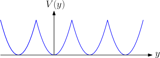
(a)

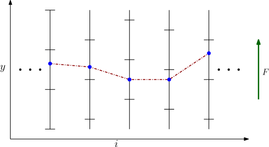
(b)

Figure 1: (color online) Illustration (a) shows the shape of the potential $V(x)$, while (b) visualizes a portion of the bi-infinite chain of particles. In (b) the particles are marked with blue dots and the “springs” connecting them are dashed red lines. The vertical black lines show the sequence of potential wells seen by particle $i$, with horizontal markings to indicate the cusps of $V$. An arrow indicates the direction of the external force $F$ exerted on the particles.

It is possible to study the dynamics of such a system, under a time-varying force, with a system of ODEs for inertialess particles under relaxational dynamics: other authors such as [27, 18, 23, 20, 19] have pursued this approach. Instead we will assume that the time scale at which the external force is changing is much larger than that associated with the relaxation of the particles, and therefore consider the approach to threshold through intermediate static configurations. Lemma 3.4 and its analogue in the dynamic case, the no passing rule of [23], indicate some manner of equivalence between these approaches.

Static configurations are those for which $\partial_{y_{i}}\mathcal{H}=0$ for all $i$:

$$-\Delta y_{i}+V^{\prime}(y_{i}-\alpha_{i})-F=0.$$ (2.3)

Here $\Delta$ denotes the discrete Laplace operator on sequences given by $\Delta y_{i}=y_{i-1}-2y_{i}+y_{i+1}$. When using the potential (2.2) it is convenient to introduce the notation

$$m_{i} \equiv\llbracket y_{i}-\alpha_{i}\rrbracket\in\mathbb{Z}$$ (2.4a)

$$\tilde{y}_{i} \equiv y_{i}-\alpha_{i}-m_{i}\in\left(-\textstyle\frac{1}{2},+\textstyle\frac{1}{2}\right];$$ (2.4b)

we refer to these as the well number and well coordinate of $y_{i}$, the former indicating which parabolic well contains the particle and the latter the displacement of the particle from the center of its well. Then (2.3) can be re-expressed as

$$(\lambda-\Delta)\bm{y}=\lambda(\bm{m}+\bm{\alpha}+F/\lambda).$$ (2.5)

As in [28], we may treat $\bm{m}$ and $\bm{\alpha}$ as given and solve this linear equation for $\bm{y}$. It is important to note, however, that the nonlinearity of this system has not disappeared, but rather it becomes a consistency condition: after computing $\bm{y}$ from $\bm{m}$, we must have $m_{i}=\llbracket y_{i}-\alpha_{i}\rrbracket$ for all $i$.

Elementary techniques for linear recurrences applied to (2.5) give a formula for $\bm{y}$:

$$y_{i}=\frac{1-\eta}{1+\eta}\sum_{j\in\mathbb{Z}}\eta^{|i-j|}(m_{j}+\alpha_{j})+\frac{F}{\lambda},$$ (2.6)

where

$$\eta=\frac{2}{2+\lambda+\sqrt{\lambda^{2}+4\lambda}}\in(0,1).$$ (2.7)

This is the unique choice for which $y_{i}$ does not grow geometrically as $|i|\to\infty$ even if $\bm{m}+\bm{\alpha}$ is bounded. Noting that $\lambda\bm{\tilde{y}}=\Delta\bm{y}+F$ from (2.5), it follows also that

$$\tilde{y}_{i}=\frac{\eta}{1-\eta^{2}}\sum_{j\in\mathbb{Z}}\eta^{|i-j|}(\Delta m_{j}+\Delta\alpha_{j})+\frac{F}{\lambda}.$$ (2.8)

Momentarily ignoring the relationship between $\bm{y}$ and $\bm{m}$, observe that increasing or decreasing the driving force $F$ affects the configuration by rigid translation. This, and the explicit formulas (2.6) and (2.8), are the advantages of the parabolic potential.

Taking a configuration (with $F=0$, for example) and increasing $F$ causes the chain of particles to rigidly translate until for some $i$ we have $\tilde{y}_{i}=\frac{1}{2}$; any further increase causes this particle to topple into the next well. See Figure 2 for illustration. For instance, if a jump occurs at site $j$, the resulting change in well coordinates is

$$\tilde{y}_{i}\to\tilde{y}_{i}-\delta_{ij}+\frac{1-\eta}{1+\eta}\eta^{|i-j|}$$ (2.9)

provided that $\tilde{y}_{i}<\frac{1}{2}$ for all $i$ after the change; otherwise, other particles will be pulled forward into their next wells. This process may terminate, resulting in a new static configuration, or continue forever, in which case we understand the configuration is no longer pinned and has entered the sliding regime.

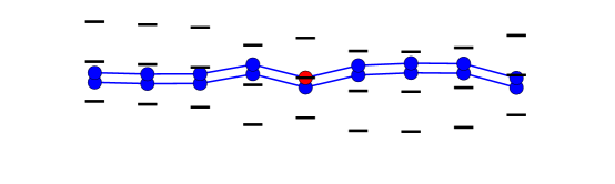
(a)

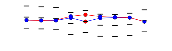
(b)

Figure 2: The configuration is (a) rigidly translated until a particle reaches the edge of its well (red) and then (b) this particle jumps into the next well, pulling all the other particles forward by an amount that decays geometrically moving away from the site that jumped.

For this model we are interested in answering the following questions:

• At what $F$ does the system depin and enter the sliding regime? We call this $F$ the threshold force and denote it $F_{\mathrm{th}}$.

• What is the shape of the configuration just before it begins to slide? As $|y_{i}-m_{i}|<1$ for all $i$ by definition, the well numbers we observe just before the threshold, $\bm{m^{+}}$, sufficiently describe the large-scale shape.

• How do various observables behave in terms of $F_{\mathrm{th}}-F$? We are particularly interested in the polarization, which is the spatial average (i.e. average over $i$) of the change in $m_{i}$ as we evolve from some initial configuration to the first configuration we encounter that is stable at the current force $F$.

In subsequent sections we present theoretical and numerical results for a finite version of this system with periodic boundary conditions. For a system with $L$ particles, we take the well numbers $m_{i}$ and the disorder $\alpha_{i}$ to be $L$-periodic sequences, the latter still i.i.d. within a single period. Our most detailed results are for an approximation we call the toy model [25]. For a strong potential, $\lambda$ is large and $\eta$ is very small, and we have

$$\tilde{y}_{i}=\eta(\Delta m_{i}+\Delta\alpha_{i})+F/\lambda+O(\eta^{2}).$$ (2.10)

Dropping the $O(\eta^{2})$ portion reduces the range of direct interactions to nearest neighbors only. In this case we can answer very explicitly all the questions posed above.

3 The avalanche algorithm

Our basic tool for both simulation and the derivation of rigorous results is the avalanche algorithm. This takes as input a static configuration, and produces a new static configuration which is stable at higher force, if possible, in a manner intended to mimic the result of increasing the force and finding the long time limiting arrangement of the particles with an inertialess dynamics. For the $L$-periodic chain in both the toy model and the model with long-range interaction, we describe this procedure in terms of the well numbers $\bm{m}$ and well coordinates $\tilde{\bm{y}}$ from (2.4a) and (2.4b).

Algorithm 3.1 (avalanche with force).

Given a valid configuration $\bm{m}$ in the environment specified by $\bm{\alpha}$ and $F$, we produce a new configuration $\bm{m}^{*}$ valid at a new $F^{*}\geq F$:

• Start with the current configuration: let $\bm{m}^{*}=\bm{m}$ (and correspondingly $\tilde{\bm{y}}^{*}=\tilde{\bm{y}}$) initially.

• Record the maximum well coordinate $\tilde{y}_{\max}=\max_{i}\tilde{y}_{i}$.

• Increase the force to $F^{*}=F+\lambda(\frac{1}{2}-\tilde{y}_{\max})$, and correspondingly adjust the well coordinates $\tilde{y}^{*}_{i}\to\tilde{y}^{*}_{i}+(\frac{1}{2}-\tilde{y}_{\max})$, bringing exactly one particle (in each period) to the cusp of the next well.

• Let $j=\operatorname*{arg\,max}_{i}\tilde{y}^{*}_{i}$ and jump particle $j$ (and its periodic equivalents) by incrementing $m^{*}_{j}\to m^{*}_{j}+1$ and suitably adjusting $\bm{\tilde{y}}^{*}$: for the full model,

  $$\tilde{y}^{*}_{i}\to\tilde{y}^{*}_{i}+\begin{cases}\displaystyle\frac{-2\eta}{1+\eta}+\frac{1-\eta}{1+\eta}\frac{2\eta^{L}}{1-\eta^{L}}&\text{for }i=j\\ \\ \displaystyle\frac{1-\eta}{1+\eta}\frac{\eta^{|i-j|}+\eta^{L-|i-j|}}{1-\eta^{L}}&\text{for }j<i<j+L\end{cases}$$ (3.1)

  and for the toy model,

  $$\tilde{y}^{*}_{i}\to\tilde{y}^{*}_{i}+\begin{cases}+1\eta&\text{for }i=j\pm 1\\ -2\eta&\text{for }i=j,\end{cases}$$ (3.2)

  and extending these periodically.

• If $\tilde{y}^{*}_{i}>1/2$ for any $i$, goto (A4).

Remark.

The formula (3.1) for updating $\tilde{\bm{y}}$ has been adapted from (2.8) to respect the periodicity. For simulation purposes we might use (2.8) unaltered, summing only over nearest periodic representatives, at the cost of an $O(\eta^{L})$ error.

For this algorithm to be well-defined, we must verify that it does, in fact, terminate. The following result indicates that it does, and gives the maximum number of jumps (A4) we might expect. It also establishes a useful property which will allow us to give a centered version of the algorithm, which is better numerically, requiring fewer floating point operations, and better theoretically, allowing us to recast the evolution in terms of a variational problem.

Proposition 3.2.

The avalanche algorithm 3.1 has the following properties:

• It terminates after finitely many steps.

• All particles jump at most once: $\bm{m}^{*}\leq\bm{m}+\bm{1}$, the inequality holding componentwise.

• If $F\geq 0$ and $\eta<1/3$, then for all $i$ the resulting configuration has

  $$\tilde{y}^{*}_{i}>-\frac{1}{2}+\frac{F^{*}-F}{\lambda}.$$ (3.3)

Property (i) is immediate from (ii), which itself follows from a consideration of (3.1) or (3.2): a particle $i$ which jumps once, decreasing $\tilde{y}_{i}$, will not see sufficient increase in $\tilde{y}_{i}$ to exceed its original height, even if all the other particles jump. Property (iii) tells us that the configuration $\bm{m}^{*}$ at force $F^{*}$ produced by the algorithm remains a valid configuration—that is, has all its well coordinates in $(-\frac{1}{2},+\frac{1}{2}]$—at the original force $F$. This illustrates that the models under consideration exhibit both reversible and irreversible behavior: increasing the force from $0$ to some $F>0$ may cause jumps, which are not undone if we reduce the force back to $0$; on the other hand, the new configuration we obtain reacts to values of the force in $[0,F]$ moving by rigid translation only, i.e. reversibly. It also allows us to write a simpler algorithm which will produce the exact same sequence of configurations.

Algorithm 3.3 (zero-force avalanche).

Given a configuration $\bm{m}$ in an environment specified by $\bm{\alpha}$ with $F=0$, produce a new configuration $\bm{m}^{*}$ valid at $F^{*}=0$:

• Let $\bm{m}^{*}=\bm{m}$.

• Record $\tilde{y}_{\max}=\max_{i}\tilde{y}_{i}$.

• Let $j=\operatorname*{arg\,max}_{i}\tilde{y}^{*}_{i}$ and jump particle $j$ (and its periodic equivalents) by incrementing $m^{*}_{j}\to m^{*}_{j}+1$ and correspondingly adjusting $\bm{\tilde{y}}^{*}$ as in (3.1) or (3.2).

• If $\tilde{y}^{*}_{i}>\tilde{y}_{\max}$ for any $i$, goto (ZFA3).

For brevity we refer to this algorithm as the ZFA. Note that the result has $\max_{i}\tilde{y}^{*}_{i}=\tilde{y}^{*}_{\max}\leq\tilde{y}_{\max}$.

Middleton’s no passing rule [23] is a monotonicity property of the inertialess ODE system used to study CDWs from a dynamic perspective: if $\bm{y}^{1}(t)$ and $\bm{y}^{2}(t)$ are two solutions to $\dot{\bm{y}}=-\nabla\mathcal{H}(\bm{y})$ where $\bm{y}^{1}(t_{0})\leq\bm{y}^{2}(t_{0})$, then $\bm{y}^{1}(t)\leq\bm{y}^{2}(t)$ for $t\geq t_{0}$. Monotonicity results are an essential tool for studying arrangements of chains of particles, even in a purely static setting. Consider, for example, the Aubry-Mather treatment of the similar Frenkel-Kontorova model, explained very nicely by Bangert [29]. That the ZFA has such a property is necessary for our subsequent observations.

Lemma 3.4 (ZFA noncrossing).

Let $\bm{m}^{1}\leq\bm{m}^{2}$ be two configurations for either the full or toy model sharing the same environment $\bm{\alpha}$, and let $\bm{m}^{1*}$ and $\bm{m}^{2*}$ be the results of applying the ZFA to each of these.

• If $\max_{i}\tilde{y}^{1}_{i}>\max_{i}\tilde{y}^{2}_{i}$, then $\bm{m}^{1*}\leq\bm{m}^{2}$.

• If $\max_{i}\tilde{y}^{1}_{i}=\max_{i}\tilde{y}^{2}_{i}$ and $m^{1}_{j}<m^{2}_{j}$ for $j=\operatorname*{arg\,max}_{i}\tilde{y}^{1}_{i}$, then $\bm{m}^{1*}\leq\bm{m}^{2}$.

• If $\max_{i}\tilde{y}^{1}\geq\max_{i}\tilde{y}^{2}_{i}$, then $\bm{m}^{1*}\leq\bm{m}^{2*}$.

In each case above, the stated conditions give a bound on the well coordinates of any particle $i$ for which $m^{1}_{i}=m^{2}_{i}$, which prevents particle $i$ from jumping in cases (i) and (ii), or shows that particle $i$ jumps for configuration 1 only if it jumps for configuration 2. The argument is very much the same as for the dynamic version [23].

We now define the threshold states for the full and toy models. Considering the above noncrossing result, the threshold configuration should be that which minimizes $\max_{i}\tilde{y}_{i}$: another configuration could not depin without first crossing this one.

Definition 3.5.

In either the full model or the toy model, for a given environment $\bm{\alpha}$, a threshold configuration is specified by well numbers $\bm{m}^{+}$ achieving

$$\min_{\bm{m}}\max_{i}\tilde{y}_{i}$$ (3.4)

where $\tilde{\bm{y}}$ is the vector of well coordinates corresponding to $\bm{m}$ at $F=0$. The threshold force is

$$F_{\mathrm{th}}=\lambda\left(\frac{1}{2}-\min_{\bm{m}}\max_{i}\tilde{y}_{i}\right).$$ (3.5)

Note that $F_{\mathrm{th}}$ is exactly the force required to bring one particle in the threshold configuration to the upper edge of its well. Here and in the sequel, we compute well coordinates from well numbers at $F=0$.

Remark.

With standard Frenkel-Kontorova, one is interested in configurations which minimize energy, which consists (in the case of Hookean springs) of an $\ell^{2}$-difference of $\bm{y}$ and its translate by one, and the terms coming from the substrate potential. Here, when considering a similar system in the presence of an increasing driving force, the relevant functional is of $\ell^{\infty}$-type.

Our next result illustrates the utility of the ZFA as we try to understand threshold behavior.

Proposition 3.6.

For both the full model and the toy model:

• The threshold configuration $\bm{m}^{+}$ exists and is almost surely unique, up to translating all components of $\bm{m}^{+}$ by the same integer.

• Starting from $\bm{m}=\bm{0}$, the ZFA finds $\bm{m}^{+}$ in finitely many steps.

• The ZFA applied to $\bm{m}^{+}$ produces $\bm{m}^{+}+\bm{1}$, and this property is unique to the family $\bm{m}^{+}+\mathbb{Z}\bm{1}$.

Existence of a minimizer in (3.4) is easy: (2.3) and periodicity can be used to bound $\max_{i}|\Delta m_{i}|$, allowing us to exclude all but a finite set of $\bm{m}$ (modulo uniform translation by integers). Uniqueness is also relatively routine, after using the noncrossing property of the ZFA to reduce possible nonuniqueness to configurations which are ordered and have well numbers differing by at most one. Noncrossing gives (ii), and the uniqueness, together with the fact that the ZFA can never increase $\max_{i}\tilde{y}_{i}$, implies (iii).

We thus have a tool, the ZFA, for both the full and toy models, which produces the threshold configuration that precedes the depinning transition. It achieves this by way of a sequence of physically meaningful intermediate states, according to an algorithm which is straightforward to implement and apply to generate numerical results. In the next section we specialize to the toy model, where more can be said.

4 The toy model: explicit formulas

In the case of the toy model we find it convenient to introduce rescaled well coordinates $\bm{z}$ defined by

$$\eta z_{i}=\tilde{y}_{i}.$$ (4.1)

As in the previous section, we fix the external force $F=0$. In this case, a jump at site $j$ as in step (iii) of Algorithm 3.3 results in

$$m_{j}\to m_{j}+1,\quad z_{j}\to z_{j}-2,\quad z_{j\pm 1}\to z_{j\pm 1}+1.$$ (4.2)

Here we find a strong similarity between the toy model and sandpile models (see [30] for an introduction), as already noted by other authors working on similar CDW systems [31, 20, 24]. Indeed, for one-dimensional sandpile models, the change to $\bm{z}$ in (4.2) is precisely the result of toppling at site $j$. The existing literature on sandpiles is extensive; see [32] for a survey, and note that models with continuous heights have been considered previously [33]. However, the authors are unable to find an exact match for the toy model in prior work. As noted in [25], the toy model has periodic boundary, conserves the sum of $\bm{z}$, evolves deterministically, changes by integers only, and preserves the fractional part of the $\Delta\bm{\alpha}$. We discuss this connection further in Section 5.

For now, the similarity between the two is a sign to expect that the toy model will permit exact results: the set of recurrent states of a standard one-dimensional sandpile is rather trivial, and one might hope that the toy model’s persistent disorder does not introduce so much complexity that things become intractable. The primary result of this section confirms this: the solution of the optimization problem posed in Definition 3.5 can be expressed explicitly.

Theorem 4.1.

Let $S=\sum_{i=0}^{L-1}\llbracket\Delta\alpha_{i}\rrbracket$. The a.s. unique threshold configuration for the toy model $\bm{m}^{+}$ satisfies

$$\Delta m^{+}_{i}=-\llbracket\Delta\alpha_{i}\rrbracket+J_{i}-\delta_{ik^{+}}$$ (4.3)

where $\bm{J}$ is an integer vector selected as follows:

• Case $S\geq 0$. $J_{i}=1$ for the $S+1$ positions $i$ which have smallest $\Delta\alpha_{i}-\llbracket\Delta\alpha_{i}\rrbracket$ and $J_{i}=0$ otherwise.

• Case $S<0$. $J_{i}=-1$ for the $|S|-1$ positions $i$ which have largest $\Delta\alpha_{i}-\llbracket\Delta\alpha_{i}\rrbracket$ and $J_{i}=0$ otherwise.

and $k^{+}$ is an index defined by

$$k^{+}=\sum_{i=0}^{L-1}i(-\llbracket\Delta\alpha_{i}\rrbracket+J_{i})\pmod{L}.$$ (4.4)

The proof is given in Section 7, and, due to Proposition 3.6, amounts to checking that $\bm{m}^{+}$ is mapped to $\bm{m}^{+}+\bm{1}$ by the ZFA. To explore the consequences of this explicit description, we first require some notation. Let

$$\epsilon_{i}=\Delta m_{i}+\llbracket\Delta\alpha_{i}\rrbracket,$$ (4.5)

and refer to those sites where $\epsilon_{i}\neq 0$ as defects with charge $\epsilon_{i}$. Write

$$\omega_{i}=\Delta\alpha_{i}-\llbracket\Delta\alpha_{i}\rrbracket$$ (4.6)

for the fractional part of $\Delta\alpha_{i}$, and let $\sigma$ be the permutation of $\{0,1,\ldots,L-1\}$ which orders $\bm{\omega}$:

$$\omega_{\sigma(0)}<\omega_{\sigma(1)}<\cdots<\omega_{\sigma(L-1)}.$$ (4.7)

Using this terminology, Theorem 4.1 gives the threshold force explicitly.

Corollary 4.2.

For the toy model, the maximum $z^{+}_{\max}$ of the rescaled well coordinates (see (4.1)) of the threshold configuration is

$$z^{+}_{\max}=\begin{cases}\omega_{\sigma(S)}+1&\text{if }S\geq 0\text{ and }k^{+}\neq\sigma(S)\\ \omega_{\sigma(S-1)}+1&\text{if }S>0\text{ and }k^{+}=\sigma(S)\\ \omega_{\sigma(L-1)}&\text{if }S=0\text{ and }k^{+}=\sigma(0)\\ \omega_{\sigma(L-|S|)}&\text{if }S<0\text{ and }k^{+}\neq\sigma(L-|S|)\\ \omega_{\sigma(L-|S|-1)}&\text{if }S<0\text{ and }k^{+}=\sigma(L-|S|),\end{cases}$$ (4.8)

and the corresponding threshold force $F_{\mathrm{th}}$ is

$$F_{\mathrm{th}}=\lambda\left(\frac{1}{2}-\eta z^{+}_{\max}\right).$$ (4.9)

Remark.

As we will see in Section 5, the cases $k^{+}\in\{\sigma(S),\sigma(L-|S|)\}$ have probability tending to 0 as the system size $L\to\infty$.

We wish to understand not only the threshold configuration but the behavior of the system as we approach it. The noncrossing property Lemma 3.4 of the ZFA implies that we may take any valid configuration and, by repeated application of this algorithm, arrive at the threshold state. During this process, we track certain quantities associated with the system’s evolution.

Of particular interest is the observable known as polarization, as this has been the subject of several previous studies in CDW and related models [15, 20, 24]. Given an initial state corresponding to some well numbers $\bm{m}^{0}$, applying the ZFA produces a sequence of configurations (essentially) terminating with $\bm{m}^{+}$. Suppose that we record these configurations, calling them $\bm{m}(\tau)$ for $\tau$ in some index set $T$. Then the polarization is the function of $\tau$ given by

$$P(\tau)\equiv\frac{1}{L}\sum_{j=0}^{L-1}(m_{j}(\tau)-m^{0}_{j}).$$ (4.10)

We write also $\Sigma(\tau)=LP(\tau)$, and call $\Sigma(\tau)$ the cumulative avalanche size. In either case, the quantity under consideration is the total number of particle jumps which have occurred in the process of evolving from the initial state $\bm{m}^{0}$ to the current state $\bm{m}(\tau)$.

Among all possible initial conditions $\bm{m}^{0}$, two seem particularly natural from a macroscopic perspective: we might begin with flat well numbers, $m^{0}_{i}=0$ for all $i$, or we might take the negative threshold configuration, $\bm{m}^{0}=\bm{m}^{-}$, defined precisely below. In the flat case we have only statistics for the complete evolution without intermediate configurations, which we discuss in Section 5. For the threshold-to-threshold evolution, on the other hand, there is a nice interpretation, in terms of record sequences, for each step of the evolution, which we develop in the remainder of this section.

For both the toy model and the full model, given a realization $\bm{\alpha}$, write $\bm{m}^{+}$ for a threshold configuration as previously defined, and call it a $(+)$-threshold configuration. Define also a $(-)$-threshold configuration $\bm{m}^{-}$, which achieves

$$\max_{\bm{m}}\min_{i}\tilde{y}_{i}$$ (4.11)

for $\tilde{y}_{i}$ the well coordinates corresponding to $\bm{m}$. (Note that this can be obtained from the $(+)$-threshold configuration with $\bm{\alpha}$ replaced with $-\bm{\alpha}$.) We can adapt (4.3) to produce the negative threshold configuration of the toy model, which maximizes $\min_{i}z_{i}$. Define $J^{-}$ and $k^{-}$ as follows:

• Case $S>0$. $J^{-}_{i}=1$ for the $S-1$ positions $i$ which have smallest $\omega_{i}$, $J^{-}_{i}=0$ otherwise;

• Case $S\leq 0$. $J^{-}_{i}=-1$ for the $|S|+1$ positions $i$ which have largest $\omega_{i}$, $J^{-}_{i}=0$ otherwise;

and $k^{-}$ is given in terms of $J^{-}$ by analogy with (4.4).

In the toy model, several successive applications of the ZFA may have initial jumps occurring at the same site. This behavior will be especially prevalent for the threshold-to-threshold evolution. It will be useful both intuitively and technically to view these transitions in aggregate. For a given non-threshold configuration $(\bm{m},\bm{z})$ with $i=\operatorname*{arg\,max}_{k}z_{k}$, let $i_{L}$ and $i_{R}$ be the indices of sites closest to $i$ on the left and right, respectively, for which

$$z_{i_{L}}+1\leq z_{i}\qquad\text{and}\qquad z_{i_{R}}+1\leq z_{i}.$$ (4.12)

Define sets of indices $W_{1},\ldots,W_{\ell}$ for $\ell=(i-i_{L})\wedge(i_{R}-i)$, by

$$W_{k}=[i_{L}+k,i_{R}-k].$$ (4.13)

Proposition 4.3.

The first $\ell$ iterations of the ZFA applied to $(\bm{m},\bm{z})$ as above cause jumps at sites with indices in $W_{1},\ldots,W_{\ell}$, respectively. We call this sequence an avalanche, the individual iterations avalanche waves, and $i_{L},i_{R}$ the left and right extents of the avalanche. (The wave terminology has been borrowed from sandpile models [34].) Throughout this process, site $i$ remains the location of the maximum, and the original $z_{i}$ the maximum value, at least until after the $\ell^{\mathrm{th}}$ iteration. It follows that

• The total number of jumps in the avalanche is $(i-i_{L})(i_{R}-i)$.

• The resulting changes in the configuration $(\bm{m},\bm{z})$ are:

  $$z_{i_{L}} \to z_{i_{L}}+1$$ (4.14a)

  $$z_{i_{R}} \to z_{i_{R}}+1$$ (4.14b)

  $$z_{i} \to z_{i}-1$$ (4.14c)

  $$z_{i_{L}+i_{R}-i} \to z_{i_{L}+i_{R}-i}-1$$ (4.14d)

  and

  $$m_{j}\to m_{j}+(j-i_{L})_{+}-(j-i)_{+}-(j-i-i_{R}+i_{L})_{+}+(j-i_{R})_{+}.$$ (4.14e)

  In the case where $i-i_{L}=i_{R}-i$, the transition at $i$ is $z_{i}\to z_{i}-2$.

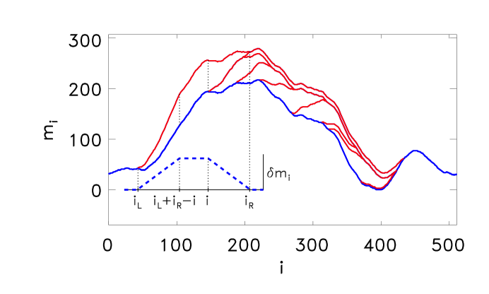
Figure 3: Evolution of $\bm{m}$ under the ZFA starting from the negative threshold configuration (blue). The sequence of intermediate configurations reached by triggering of avalanches is shown in red. The topmost configuration is the positive threshold configuration. The inset displays the trapezoidal change resulting from one of the avalanches.

Note the change $\delta\bm{m}$ in $\bm{m}$ shown in (4.14e) is trapezoidal. Figure 3 displays the changes resulting from several avalanches. To illustrate the threshold-to-threshold evolution for the toy model, it is convenient to introduce

$$\zeta_{i}=\omega_{i}+J^{-}_{i}$$ (4.15)

and the permutation $\pi$ that orders $\zeta$:

$$\zeta_{\pi(0)}<\zeta_{\pi(1)}<\cdots<\zeta_{\pi(L-1)}.$$ (4.16)

Note $\zeta_{\pi(L-1)}-\zeta_{\pi(0)}<1$. The $(\pm)$-threshold configurations have

$$z^{-}_{i} =\zeta_{i}+\delta_{ik^{-}}$$ (4.17)

$$z^{+}_{i} =\zeta_{i}+\delta_{i\pi(0)}+\delta_{i\pi(1)}-\delta_{ik^{+}},$$ (4.18)

and, using the divisibility condition (4.4), $k^{\pm}$ are related by

$$k^{+}=\pi(0)+\pi(1)-k^{-}.$$ (4.19)

Observe that the ranks $\pi^{-1}$ of the $\bm{\zeta}$ suffice to determine an avalanche’s initial site and extents. We represent a given configuration $z_{j}$ by displaying the rank $\pi^{-1}(j)$ of $\zeta_{j}$ and using over- or underlines to indicate additions by $\pm 1$ which are acquired as a result of jumps:

$$\overline{s} \leftrightarrow z_{\pi(s)}=\zeta_{\pi(s)}+1,$$ (4.20)

$$\underline{s} \leftrightarrow z_{\pi(s)}=\zeta_{\pi(s)}-1.$$

As in [25], an example clarifies things. Suppose that $z^{-}$ has the rank representation

$$\begin{array}[]{cccccccccccc}\ldots&0&10&12&17&\overline{15}&16&18&11&13&1&\ldots\end{array}$$

so that $k^{-}=\pi(15)$. The extents of the first avalanche are $k^{-}-i_{L}=2,i_{R}-k^{-}=3$ and after the sites bracketed below have jumped, the resulting configuration is

$$\begin{array}[]{cccccccccccc}\ldots&0&10&\overline{12}&[\underline{17}&\overline{15}&16&\underline{18}]&\overline{11}&13&1&\ldots.\end{array}$$

In the second wave, $k^{-}$ and $k^{-}+1$ jump again, yielding

$$\begin{array}[]{cccccccccccc}\ldots&0&10&\overline{12}&17&[15&\underline{16}]&18&\overline{11}&13&1&\ldots,\end{array}$$

and the avalanche is complete. The remaining avalanches begin at the sites ranked $12$, $11$, and $10$; the result is the positive threshold configuration.

This example illustrates that the important sites in the threshold-to-threshold evolution are the lower records [35, 36]: given a sequence of values $X_{1},X_{2},\ldots$, we say that $X_{i}$ is a lower record if $X_{i}=\min\{X_{j}:j\leq i\}$. Using (4.12) and Proposition 4.3 we see that avalanches are determined by the locations of the lower records of the sequences

$$\mathcal{J}_{L} =\zeta_{k^{-}},\zeta_{k^{-}-1},\zeta_{k^{-}-2},\ldots,\zeta_{\pi_{L}},$$ (4.21)

$$\text{and}\quad\mathcal{J}_{R} =\zeta_{k^{-}},\zeta_{k^{-}+1},\zeta_{k^{-}+2},\ldots,\zeta_{\pi_{R}},$$ (4.22)

where $\{\pi_{L},\pi_{R}\}=\{\pi(0),\pi(1)\}$ are the termination sites. The evolution from negative to positive threshold terminates when the avalanches reach $\pi_{L}$ and $\pi_{R}$.

We are most interested in the dependence of the polarization on $F_{\mathrm{th}}-F$, the difference between the current force and that at $(+)$-threshold. For the zero-force description, the quantity that serves this purpose is $X\equiv z_{\max}-z^{+}_{\max}$, the maximum height of the current configuration minus that of the $(+)$-threshold configuration. We parametrize the configurations we see in the threshold-to-threshold evolution by a nonnegative real quantity $x$: $\bm{m}(x)$ is the first configuration we see for which $X\leq x$. Note that this has the effect of skipping over the results of the individual avalanche waves, because only complete avalanches give a strict decrease in $X$.

By shifting indices, we can make $k^{-}=0$; let $j_{L}(x)$ and $j_{R}(x)$ be the (noninclusive) left and right extents of the interval of sites which have jumped in order to achieve $X\leq x$. We select

$$-L+j_{R}(x)<j_{L}(x)\leq 0\leq j_{R}(x)<j_{L}(x)+L.$$ (4.23)

Note that $j_{L}(x)$ and $j_{R}(x)$ are indices of the lower records from the sequences (4.21) and (4.22), respectively. In the threshold-to-threshold evolution, $j_{L}(x)$ and $j_{R}(x)$ are sufficient to characterize the shape of $\bm{m}(x)-\bm{m}^{0}$, because this remains trapezoidal. This follows because

• the result of any complete avalanche is a trapezoidal change, and

• for the threshold-to-threshold evolution, starting with an overall trapezoidal change, the next avalanche is initiated at one of its convex corners, and terminates on one side at one of the concave corners.

Then the corresponding cumulative avalanche size $\Sigma(x)$ and polarization $P(x)$ are

$$\Sigma(x) =-j_{L}(x)j_{R}(x)$$ (4.24)

$$P(x) =\frac{\Sigma(x)}{L}.$$ (4.25)

To understand the threshold-to-threshold polarization as a function of $F_{\mathrm{th}}-F$ amounts to understanding the statistics of the pair $j_{L},j_{R}$. This and other probabilistic questions are addressed in the next section.

5 Statistical results

We begin by characterizing the variates $\omega_{i}=\Delta\alpha_{i}-\llbracket\Delta\alpha_{i}\rrbracket$ introduced previously, as the $(\pm)$-threshold configurations are explicit functions of these. The following proposition is not interesting itself, but gives some indication how the choice we have made for the disorder enables the subsequent results.

Proposition 5.1.

The variates $\omega_{i}=\Delta\alpha_{i}-\llbracket\Delta\alpha_{i}\rrbracket$, $i=0,\ldots,L-1$, have the joint distribution that results from taking i.i.d. uniform $(-\frac{1}{2},+\frac{1}{2})$ variates and conditioning them to sum to an integer; by this we mean $\bm{\omega}$ is distributed according to the (normalized) surface measure on the intersection of the cube $(-\frac{1}{2},+\frac{1}{2})^{L}$ with the family of planes $x_{0}+x_{1}+\cdots+x_{L-1}\in\mathbb{Z}$.

Using the above it is easy to check that the one-dimensional marginals are uniform $(-\frac{1}{2},+\frac{1}{2})$, and while $\{\omega_{i}\}_{i=0}^{L-1}$ are dependent, removing just one of these is enough to restore independence. We apply the central limit theorem for $L-1$ of these, and note that the variate omitted can alter the sum by at most $\frac{1}{2}$.

Corollary 5.2.

The sum $S=\sum_{i=0}^{L-1}\llbracket\Delta\alpha_{i}\rrbracket$, and hence the number of topological defects, behave as follows as $L\to\infty$.

• As $L\to\infty$,

  $$L^{-1/2}S=L^{-1/2}\sum_{i=0}^{L-1}\llbracket\Delta\alpha_{i}\rrbracket$$ (5.1)

  converges in distribution to a normal random variable with mean 0 and variance $1/12$.

• The typical number of topological defects (sites where $\epsilon_{i}=\Delta m_{i}+\llbracket\Delta\alpha_{i}\rrbracket\neq 0$) scales like $L^{1/2}$.

We observe also numerically that as $L\to\infty$, $\mathbb{E}F_{\mathrm{th}}\to\frac{\lambda}{2}(1-\eta)$ and $L^{1/2}(F_{\mathrm{th}}-\mathbb{E}F_{\mathrm{th}})$ converges in distribution to a Gaussian with mean 0 and variance $(12L)^{-1}$

The rescaled well coordinates $\bm{z}^{+}$ at threshold are obtained by the modification of $\bm{\omega}$ described in (4.3) and (4.4). This modification does not preserve all the properties of $\bm{\omega}$, but a particularly important one is left intact.

Theorem 5.3.

The components $z^{+}_{i}$ of the vector $\bm{z}^{+}$ of centered, rescaled well-coordinates at threshold are exchangeable.

This leads quickly to a nice macroscopic description of the threshold configurations as $L\rightarrow\infty$. First, some physical motivation: the strains, which are the magnitudes of the forces exerted by springs connecting the particles, are expected to diverge at threshold [12, 13] in CDW systems. This is possible because we have assumed that the interaction between the particles can survive any stress applied to it. This is of course unphysical and one expects that beyond a certain strain, plastic effects become dominant. In the case of CDW systems, this plasticity gives rise to phase slips: the springs yield once the strain reaches a certain value. If we intend to use the toy model to better understand such behavior, we need to understand how the strains build up as a function of the external force. At present, we can at least characterize the strains at threshold in a precise way.

Write $s_{i}=m_{i+1}-m_{i}$, $i=0,\ldots,L-1$, for the strains in the configuration indicated by $\bm{m}$. Also let

$$s^{(L)}(t)\equiv(12/L)^{1/2}s_{\lfloor Lt\rfloor}\quad(0\leq t\leq 1)$$ (5.2)

be the càdlàg process obtained from $\bm{s}$ after central limit rescaling. A well known limit theorem for exchangeable variates (found for instance in [37]) gives the distributional limit of the processes $s^{(L)}$.

Corollary 5.4.

With $\bm{m}=\bm{m}^{+}$ and the corresponding threshold strains $\bm{s}$, as $L\to\infty$ the processes $s^{(L)}$ converge distributionally in the Skorokhod space $\mathcal{D}([0,1])$ (equipped with the $J_{1}$-topology) to a periodic Brownian motion with zero integral:

$$B_{0}(t)\equiv B(t)-\int_{0}^{1}B(r)\,dr\quad(0\leq t\leq 1),$$ (5.3)

where $B(t)$ is a standard Brownian bridge. The process $B_{0}$ is Gaussian with zero mean, stationary under periodic translations of the interval $[0,1]$, with covariance given by

$$\mathbb{E}B_{0}(0)B_{0}(t)=\frac{1}{12}(1-6t+6t^{2})\qquad(0\leq t\leq 1).$$ (5.4)

Simulations of full CDW systems [15, 24] suggest that the total threshold-to-threshold polarization scales like $P\sim L^{3/2}$. The scaling limit of Corollary 5.4 allows us to deduce this scaling for the total polarization from flat initial condition to threshold. We compute

$$P=\frac{1}{L}\sum_{i=0}^{L-1}m^{+}_{i} =\int_{0}^{1}m^{+}_{\lfloor Lt\rfloor}\,dt=\int_{0}^{1}\left\{\sum_{i=0}^{\lfloor Lt\rfloor}s_{i}-\min_{0\leq r\leq 1}\sum_{i=0}^{\lfloor Lr\rfloor}s_{i}\right\}\,dt$$

$$=L\int_{0}^{1}\left\{\int_{0}^{t}s_{\lfloor Lu\rfloor}\,du-\min_{0\leq r\leq 1}\int_{0}^{r}s_{\lfloor Lu\rfloor}\,du\right\}\,dt$$

$$=L^{3/2}\left\{\int_{0}^{1}\int_{0}^{t}L^{-1/2}s_{\lfloor Lu\rfloor}\,du\,dt-\min_{0\leq r\leq 1}\int_{0}^{r}L^{-1/2}s_{\lfloor Lu\rfloor}\,du\right\}$$

$$=\frac{L^{3/2}}{\sqrt{12}}\left\{\int_{0}^{1}s^{(L)}(t)(1-t)\,dt-\min_{0\leq r\leq 1}\int_{0}^{r}s^{(L)}(t)\,dt\right\}$$

The functional on $\mathcal{D}([0,1])$ given by

$$\psi(t)\mapsto\int_{0}^{1}\psi(t)(1-t)\,dt-\min_{0\leq r\leq 1}\int_{0}^{r}\psi(t)\,dt$$ (5.5)

is continuous, so this yields a distributional limit for $L^{-3/2}P$.

The distributional limit for $\sqrt{12/L^{3}}P$ can be re-expressed in terms of Brownian bridge:

$$\int_{0}^{1}B_{0}(t)(1-t)\,dt-\min_{0\leq r\leq 1}\int_{0}^{r}B_{0}(t)\,dt=\max_{0\leq r\leq 1}\int_{0}^{1}B(t)(\textstyle\frac{1}{2}-(t-r)-\mathbf{1}_{(0,r)}(t))\,dt.$$ (5.6)

Writing $\phi(t)=\frac{1}{2}-t$ for $0\leq t\leq 1$, and extending so that $\phi$ is $1$-periodic, the desired distribution is that of

$$\max_{0\leq r\leq 1}\int_{0}^{1}B(t)\phi(t-r)\,dt=\max_{0\leq r\leq 1}\int_{0}^{1}B(t+r)\phi(t)\,dt,$$ (5.7)

extending $B(t)$ to be $1$-periodic. Noting that $B(\cdot+r)-B(r)$ has the same distribution as $B(\cdot)$, and that $\phi(t)$ is orthogonal to constant functions, we find that

$$G(r)=\int_{0}^{1}B(t)\phi(t-r)\,dt$$ (5.8)

is a mean zero, stationary Gaussian process. A straightforward calculation gives

$$\mathbb{E}G(0)G(r)=\frac{1}{720}(1-30r^{2}+60r^{3}-30r^{4})\qquad(0\leq r\leq 1).$$ (5.9)

In particular, $\mathbb{E}(G(r)-G(0))^{2}\sim r^{2}$ as $r\to 0$, and a result of Weber [38] applies to show there exists a constant $c>0$ so that

$$c^{-1}t\sqrt{720}\Psi(t\sqrt{720})\leq\mathbb{P}\left\{\max_{0\leq r\leq 1}G(r)>t\right\}\leq ct\sqrt{720}\Psi(t\sqrt{720})$$ (5.10)

for all $t\geq 0$. Here $\Psi(x)$ is the probability that a standard normal random variable exceeds $x$. It follows that the distributional limit of $L^{-3/2}P$ has sub-Gaussian tail. We are unable to describe the distribution more precisely, and in general distributions of maxima of Gaussian processes are known explicitly in only a handful of cases [39]. See Figure 4 for simulation results.

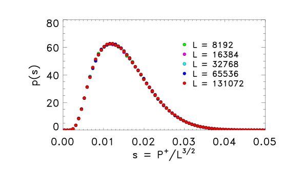
Figure 4: Simulated distribution for the flat-to-threshold polarization, rescaled by $L^{-3/2}$, for various $L$. The distributions were obtained from $10^{6}$ random realizations for each size.

For the threshold-to-threshold polarization in the toy model, our description is considerably more detailed: instead of a single quantity $P$, we have a function $P(x)$ defined in (4.25) with a parameter $x$ indicating how close we are to the threshold ($x=0$). Interestingly, the threshold-to-threshold polarization $P(0)\sim L$, not $L^{3/2}$.

Relating the following proposition to the genuine $P(x)$ requires an approximation which remains, at the moment, unjustified, but the result seems reasonable and matches very well our simulations.

Proposition 5.5.

Approximate $\mathcal{J}_{L}$ and $\mathcal{J}_{R}$ from (4.21) and (4.22) with i.i.d. uniform $(-\frac{1}{2},+\frac{1}{2})$ variates sharing their first elements. Writing $x=u/L$, we obtain the finite-size scaling function $\Phi(u)$ for the cumulative avalanche size:

$$\Phi(u)\equiv\lim_{L\to\infty}L^{-2}\mathbb{E}[\Sigma(u/L)]=\frac{6-4u+u^{2}-6e^{-u}-2ue^{-u}}{u^{4}}.$$ (5.11)

This is the result of averaging the distributional limit $\varsigma(u)\equiv\lim_{L\to\infty}\Sigma(u/L)/L^{2}$, which has density $p_{u}(s)=\mathbb{P}(\varsigma(u)\in ds)/ds$ given by

$$p_{u}(s)=\int_{2\sqrt{s}}^{1}dz\,e^{-zu}\frac{4+8u(1-z)+2u^{2}(1-z)^{2}}{(z^{2}-4s)^{1/2}},$$ (5.12)

with support on the interval $[0,\frac{1}{4}]$.

Some remarks are needed to interpret this result. First note that there is no singularity in (5.11): writing series for the exponentials,

$$\Phi(u)=\frac{1}{12}-\frac{u}{30}+\frac{u^{2}}{120}-\frac{u^{3}}{105}+O(u^{4})$$ (5.13)

for $0<u\ll 1$. For $u\gg 1$ we have

$$\Phi(u)\sim u^{-2}.$$ (5.14)

Noting the definition (5.11), this shows that $\Sigma$ (and not $P$, [25]) exhibits finite size scaling behavior: i.e. the graphs of $L^{-2}\mathbb{E}[\Sigma]$ vs. $u=XL$ for various $L$ asymptotically collapse to the graph of a the scaling function $\Phi(u)$ and moreover, in the scaling regime $u\gg 1$, the dependence on $L$ drops out. This is indeed confirmed by the results of numerical simulations shown in Figure 5. The finite size scaling behavior implies that the correlation length $\xi$ scales as

$$\xi=X^{-1}.$$ (5.15)

In terms of the underlying record process we can motivate this as follows. Given a current record $X$, the next record will occur on average after $1/X$ sites. Since all sites within this range are forced to jump once the current record site initiates the next avalanche, this defines the correlation length $\xi\sim X^{-\nu}$, with exponent $\nu=1$. The crossover to the saturated regime occurs when $\xi$ is comparable to $L$, namely $u=XL\sim L/\xi\sim 1$. From (4.24), the cumulative avalanche size is the product of the left and right extents of sites which have jumped, and thus scales as $X^{-2}$. This exponent is traditionally denoted as $-\gamma+1$ [11, 24], so that $\gamma=3$. The crossover behavior is clearly seen in Figure 5.

Figure 5: Numerical results for the expected cumulative jump size $\Sigma(X)$ vs. the reduced and rescaled force, $u=XL$, in the evolution from the negative to positive threshold configuration. Symbol colors refer to different system sizes $L$, as indicated in the legend, with accompanying numbers of realizations in parentheses. The blue dashed line indicates a power-law with exponent $-2$, while the black line is the horizontal asymptote $\mathbb{E}({\Sigma})L^{-2}=1/12$. The solid line is the theoretical finite-size scaling function, $\Phi(u)$, (5.11).

Two observations can be made about the distribution of $\varsigma(u)$. We first identify a rescaling demonstrating its scale-free behavior within the scaling regime, and then simplify (5.12) in the case $u=0$. In each case, the results take familiar forms. Making a change of variable

$$t=uz-2u\sqrt{s},$$

the integral (5.12) becomes

$$p_{u}(s)=e^{-2u\sqrt{s}}\,\int_{0}^{u(1-2\sqrt{s})}dt\,e^{-t}\,\frac{4+8(u-t-2u\sqrt{s})+2(u-t-2u\sqrt{s})^{2}}{\sqrt{t(t+4u\sqrt{s})}}.$$ (5.16)

Scaling $\varsigma(u)$ such that

$$\lim_{u\rightarrow\infty}u^{2}\varsigma(u)\equiv\mathfrak{a},$$ (5.17)

the right endpoint of the interval of integration in (5.16) tends to $\infty$, and the numerator of the fraction in the integrand is $2u^{2}$ to leading order. By dominated convergence as $u\to\infty$, the density $p(a)=\mathbb{P}(\mathfrak{a}\in da)$ of the rescaled avalanche size $\mathfrak{a}$ is

$$p(a)=2\,e^{-2\sqrt{a}}\,\int_{0}^{\infty}dt\,\frac{e^{-t}}{\sqrt{t(t+4\sqrt{a})}}=2{\rm K_{o}}(2\sqrt{a}),$$ (5.18)

where ${\rm K_{o}}$ is the modified Bessel Function, which decays at large values of its argument as $e^{-2\sqrt{a}}/(2\sqrt{a})^{1/2}$. For the $u$-values shown in Figure 6, the asymptotic form (5.18) is indistinguishable from the exact result (5.12), explaining the collapse of the data. The form of the scaling variable $a$ can be understood by noting that $a=u^{2}s=X^{2}\Sigma=\Sigma/\xi^{2}$; thus the avalanche sizes are measured in units of $\xi^{2}$.

Figure 6: Numerical cumulative avalanche size distribution for various $L$ and $u$. For large $u$, the distributions collapse when avalanche sizes are scaled as $a=u^{2}s$. The solid line is (5.12). Symbol colors refer to different $L$, as indicated in the legend and the numbers of realizations are shown in parentheses. Symbol shapes refer to the different values of $u$ chosen.

Next, the density $p_{0}(s)$ for the complete threshold-to-threshold polarization simplifies,

$$p_{0}(s)=2\ln\frac{1+\sqrt{1-4s}}{1-\sqrt{1-4s}}.$$ (5.19)

The distribution (5.19) matches exactly the avalanche size distribution of Dhar’s Abelian sandpile model in 1d [40, 41, 42]. This is not a coincidence, as we now explain.

In the sandpile model, the height parameter $h_{i}$ can take only nonnegative integer values, and is stable only if $h_{i}\in\{0,1\}$ for all $i$. Given a 1d sandpile of length $\mathcal{L}$ with sites labeled $1$ to $\mathcal{L}$ and some stable initial configuration, a site $i$ is selected at random and a grain of sand is added so that $h_{i}\rightarrow h_{i}+1$. The toppling rules of the model are as follows:

• Find any $j$ such that $h_{j}\geq 2$, set $h_{j}\to h_{j}-2$, and $h_{j\pm 1}\to h_{j\pm 1}+1$.

• If $h_{i}\geq 2$ for some $i$, goto (i).

It is useful to add pockets, sites $i=0$ and $i=\mathcal{L}+1$, which we do not consider as part of the sandpile. One of the grains which topples from site $1$ or $\mathcal{L}$ will fall into a pocket and is lost. We fix $h_{0}=h_{\mathcal{L}+1}=0$.

The set of recurrent states $\mathcal{R}$ consists of the $\mathcal{L}+1$ configurations which have $h_{i}=1$ for all but at most one site (where it is $0$). It can be shown [40, 41, 30] that:

• Starting with any configuration in $\mathcal{R}$ and adding $1$ at any site, the sandpile algorithm produces a result in $\mathcal{R}$.

• Under dynamics which consist of adding $1$ at a site chosen uniformly at random and stabilizing, the uniform distribution on $\mathcal{R}$ is invariant.

• Starting with a recurrent state and adding at site $k$ with $h_{k}=1$, the active region where topplings occur is the interval containing $k$ bounded by the closest sites $i$, possibly pockets, to the left and right of $k$ at which $h_{i}=0$. As the boundaries $\sigma_{L},\sigma_{R}$ are excluded from the interval for the toy model, so are the boundaries where $h_{i}=0$ excluded from the active region.

As we have seen in the previous sections, the evolution under the ZFA is a dynamics of moving over- or underlines in the rank diagram. In the negative threshold configuration of the toy model we encounter three types of sites, those with an overbar (corresponding to $h=2$ sites), those without a bar ($h=1$ sites), and those with an underbar ($h=0$ sites). After aligning the active regions of both models, which have identical size if we set $\mathcal{L}=L-2$, we obtain a correspondence between a negative threshold configuration of the toy model and a recurrent state of the sandpile.

We observe also the equivalence of the total threshold-to-threshold evolution of the toy model and the stabilization of a recurrent sandpile configuration when a single grain is added. The key point is that the totality of the iterated ZFA evolution is Abelian [25]. If we set $z^{+}_{\rm max}=\max_{j}z^{+}_{j}$, the maximum height of the positive threshold configuration, and then jump all sites which have $z_{j}>z^{+}_{\rm max}$, then:

• all particles in the active region will be forced to jump at least once,

• the order in which those sites with $z_{j}>z^{+}_{\max}$ are jumped is immaterial if we are concerned only with the final result, and

• the positive threshold configuration is ultimately reached.

This is equivalent to running the BTW/Dhar sandpile algorithm on the sites with overbars, which preserves the correspondence between sandpile and toy model configurations. However, this map discards the ordering and values of the well coordinates $z_{i}$, which in turn drive the evolution towards threshold in the ZFA and thereby give rise to a family of distributions (5.12).

6 Numerics

The toy model ZFA has a very fast numerical implementation which we now describe. For the threshold-to-threshold evolution, the negative threshold configurations are generated following (4.11), and the random permutation $\pi$ from (4.16) is obtained. The evolution proceeds in units of avalanches using Proposition 4.3(iii) and the rank representation of configurations, as outlined in the discussion following the proposition. We therefore only have to keep track of the locations of the over- and underlines which involves simple integer arithmetic. This implementation is fast, since instead of individual jumps we deal with avalanches and the expected number of avalanches occurring during threshold-to-threshold evolution turns out to scale as $\ln L$, which is what one expects, since a record breaking process underlies the evolution from negative to positive threshold. An explicit formula for the distribution of the number of steps can be derived [43].

At the end of each avalanche we record various statistics, such as the maximum of $z_{i}$, the cumulative number of jumps that have occurred at a given site, and the size of the current avalanche. All numerical results presented here were obtained without parallelization on single processors of an HP Z800 workstation. The longest run of about 262000 realizations of a size $L=131072$ system took 4 hours.

The control parameter for the approach to threshold is the difference between the sample-dependent threshold force $F_{\rm th}$ and the current force $F$. For the ZFA, which holds the force fixed at 0, the appropriate parameter is

$$X=\max_{i}z_{i}-\max_{i}z^{+}_{i}=\max_{i}z_{i}-\zeta_{\pi(1)},$$ (6.1)

where the last equality follows from (4.18).

The values of $X$ are recorded at the end of each avalanche. In the course of threshold-to-threshold evolution, we obtain a decreasing sequence $X_{\tau}$ of $X$ values, where $\tau$ indexes the avalanches. Following the definition of the corresponding processes, (7.59b), if we want to obtain statistics for a particular value $x$, the contributing avalanches $\tau$ will be those which satisfy $X_{\tau}\leq x<X_{\tau-1}$, since the corresponding configuration driven under an external force could have been translated by this amount $x$ without incurring any particle jumps. This is how the $x$-dependent avalanche size distributions and their expectation values have been obtained in Figures 5 and 6.

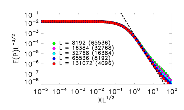
Figure 7: Numerical results for the expected cumulative jump size $P(X)$ vs. the reduced and rescaled force $u=XL$ in the evolution to threshold, starting from flat initial conditions, $\bm{m}=\bm{0}$. Colors refer to different system sizes $L$, as indicated in the legend, with accompanying numbers of realizations in parentheses. The dashed line is a power law with exponent $-3$.

We have also simulated the evolution from a flat initial configuration, $\bm{m}=\bm{0}$, to positive threshold. The evolution proceeds again by avalanches and Figure 7 shows our numerical results. The curves for different system sizes collapse for values of $u=XL<10$ under the scaling of the axes as indicated in the figure. The scaling of $P$ with $L^{-3/2}$ at $u=0$ is in agreement with the prediction following Corollary 5.4. The scaling of the abscissa as $XL^{1/2}$ suggests that the correlation lengths $\xi$ scales now as $\xi\sim X^{-2}$. We return to a discussion of this result in the conclusion.

7 Proofs

In this section we provide proofs for the results stated in the preceding text, in order of appearance.

Proposition 3.2.

That (i) the number of jumps is finite, and in fact bounded by $L$, is immediate from (ii) $\bm{m}^{*}\leq\bm{m}+1$, so we proceed to the latter. We argue inductively: suppose that after some execution of (A4) we have well numbers $\bm{m}^{\prime}$ and well coordinates $\bm{\tilde{y}}^{\prime}$, and that $\bm{m}^{\prime}\leq\bm{m}+1$. If $\max_{i}\tilde{y}^{\prime}_{i}\leq 1/2$ we are done, so suppose that $\tilde{y}^{\prime}_{k}>1/2$ for some index $k$. We claim $m^{\prime}_{k}=m_{k}$, i.e. site $k$ has not yet jumped. For the full model, observe that the jump response (3.1) has

$$\left[\frac{-2\eta}{1+\eta}+\frac{1-\eta}{1+\eta}\frac{2\eta^{L}}{1-\eta^{L}}\right]+\sum_{i=1}^{L-1}\left[\frac{1-\eta}{1+\eta}\frac{\eta^{i}+\eta^{L-i}}{1-\eta^{L}}\right]=0.$$ (7.1)

It follows that any particle which has jumped has well coordinate at most what it was after (A3), namely $1/2$. For the toy model, a site which has jumped once with neighbors which have each jumped at most once has no increase beyond its value after (A3). In either case, $m^{\prime}_{k}=m_{k}$ follows, and $\bm{m}^{\prime}+\bm{\delta}_{k}\leq\bm{m}+1$.

For (iii), if a given site $i$ has not jumped, then $\tilde{y}^{*}_{i}$ is obtained from $\tilde{y}_{i}>-1/2$ by translating upward $(F^{*}-F)/\lambda$ and then adding the (positive) effects of jumps at the other sites. So there is nothing to check unless the site $i$ has jumped. In this case,

$$\tilde{y}_{i}+\frac{F^{*}-F}{\lambda}+a>+\frac{1}{2}$$ (7.2)

with $a$ the (positive) effect of the jumps at other sites which have preceded the jump at $i$, and

$$\tilde{y}^{*}_{i} =\tilde{y}_{i}+\frac{F^{*}-F}{\lambda}+a-\left(\frac{2\eta}{1+\eta}-O(\eta^{L})\right)$$

$$>\frac{1}{2}-\frac{2\eta}{1+\eta}$$

$$=\frac{F^{*}-F}{\lambda}+\frac{1}{2}-\frac{F^{*}-F}{\lambda}-\frac{2\eta}{1+\eta}.$$

So we require

$$\frac{F^{*}-F}{\lambda}+\frac{2\eta}{1+\eta}<1.$$ (7.3)

Since $F\geq 0$, one can easily verify from (2.8) that the sum of the well coordinates $\tilde{y}_{i}$ is nonnegative regardless of $\bm{m}$. Thus values of $F^{*}$ with $(F^{*}-F)/\lambda>1/2$ can correspond only to the sliding state, and (as the avalanche algorithm produces only static configurations) we may restrict ourselves to $(F^{*}-F)/\lambda\leq 1/2$. The choice $\eta<1/3$ makes $2\eta/(1+\eta)<1/2$. The desired inequality follows. ∎

Lemma 3.4.

Suppose we are applying ZFA to $\bm{m}^{1}$ and that $\bm{m}^{\prime}$ is either equal to $\bm{m}^{1}$ or an intermediate configuration obtained after some execution of (ZFA3) for which $\bm{m}^{1}\leq\bm{m}^{\prime}\leq\bm{m}^{2}$. For any $j$ such that $m^{\prime}_{j}=m^{2}_{j}$,

$$\tilde{y}^{\prime}_{j} =\frac{1-\eta}{1+\eta}\sum_{i\in\mathbb{Z}}\eta^{|i-j|}(m^{\prime}_{i}-m^{\prime}_{j}+\alpha_{i}-\alpha_{j})$$

$$\leq\frac{1-\eta}{1+\eta}\sum_{i\in\mathbb{Z}}\eta^{|i-j|}(m^{2}_{i}-m^{2}_{j}+\alpha_{i}-\alpha_{j})=\tilde{y}^{2}_{j}$$

in the case of the full model, and

$$\tilde{y}^{\prime}_{j} =\eta(m^{\prime}_{j-1}-2m^{\prime}_{j}+m^{\prime}_{j+1})$$

$$\leq\eta(m^{2}_{j-1}-2m^{2}_{j}+m^{2}_{j+1})=\tilde{y}^{2}_{j}$$

for the toy model.

If (i) $\max_{i}\tilde{y}^{1}_{i}>\max_{i}\tilde{y}^{2}_{i}$, then $\tilde{y}^{\prime}_{j}<\max_{i}\tilde{y}^{1}_{i}$, and site $j$ will not jump. Thus the next iteration of (ZFA3), if any, will produce $\bm{m}^{\prime\prime}$ which still has $\bm{m}^{\prime\prime}\leq\bm{m}^{2}$.

If (ii) $\max_{i}\tilde{y}^{1}_{i}=\max_{i}\tilde{y}^{2}_{i}$, then $\tilde{y}^{\prime}_{j}\leq\max\tilde{y}^{1}_{i}$ and site $j$ will only jump if $\bm{m}^{\prime}=\bm{m}^{1}$, i.e. in (ZFA1), and $j=\operatorname*{arg\,max}_{i}\tilde{y}^{1}_{i}$. If $m^{1}_{j}<m^{2}_{j}$, this jump does not cause a crossing.

Since $\bm{m}^{2}\leq\bm{m}^{2*}$ and $\max_{i}\tilde{y}^{2}_{i}\geq\tilde{y}^{2*}_{i}$ trivially, and having established (i) and (ii), for (iii) we need only consider the case where

$$\max_{i}\tilde{y}^{1}_{i}=\max_{i}\tilde{y}^{2*}_{i}=\max_{i}\tilde{y}^{2}_{i}$$ (7.4)

and $m^{1}_{j}=m^{2}_{j}$ for $j=\operatorname*{arg\,max}_{i}\tilde{y}^{1}_{i}$. As in the proof of (i), we find $\tilde{y}^{1}_{j}\leq\tilde{y}^{2}_{j}$, so $j=\operatorname*{arg\,max}_{i}\tilde{y}^{2}_{i}$ as well, so that $m^{2*}_{j}=m^{2}_{j}+1>m^{1}_{j}$. Invoking (ii), we are done. ∎

Proposition 3.6.

(i) For existence, recall from (2.8) that the well coordinates can be expressed in terms of the Laplacians $\Delta\bm{m}$ and $\Delta\bm{\alpha}$. We know that $\sum_{i=0}^{L-1}\Delta m_{i}=0$, so large negative values of $\Delta m_{i}$ will require also large positive values elsewhere. The equation (2.3) (at $F=0$) can be rewritten as

$$\lambda\tilde{y}_{i}=\Delta m_{i}+\Delta\alpha_{i}+\Delta\tilde{y}_{i}.$$ (7.5)

Noting that $|\Delta\alpha_{i}|$ and $|\Delta\tilde{y}_{i}|$ are bounded by $2$, we see that large positive values of $\Delta m_{i}$ will cause large positive values of $\tilde{y}_{i}$. We may therefore optimize over $\Delta\bm{m}$ uniformly bounded above by $8$ (since anything above this is guaranteed to be worse than taking $\bm{m}=0$) and thus below by $8L$, and there are only finitely many possibilities. Existence is immediate.

Uniqueness requires separate arguments for the full model and the toy model. For the full model, suppose we have $\bm{m}^{1}$ and $\bm{m}^{2}$ threshold configurations which do not differ by simple translation. Since overall translation does not affect Laplacians, it doesn’t affect well coordinates, so we may as well assume $\min_{i}m^{2}_{i}-m^{1}_{i}=0$ and $\bm{m}^{1}\neq\bm{m}^{2}$.

We first argue that it suffices to consider $\bm{m}^{2}\leq\bm{m}^{1}+\bm{1}$. Apply the ZFA to $\bm{m}^{1}$, producing $\bm{m}^{1*}$, also a threshold configuration, and $\bm{m}^{1*}\leq\bm{m}^{1}+\bm{1}$. Write $j_{1}=\operatorname*{arg\,max}_{i}\tilde{y}^{1}_{i}$. If $m^{1}_{j}<m^{2}_{j}$, we have $\bm{m}^{1*}\leq\bm{m}^{2}$ by Lemma 3.4. We rule out $m^{1}_{j}=m^{2}_{j}$ because it forces

$$\tilde{y}^{2}_{j}>\tilde{y}^{1}_{j}=\max_{i}\tilde{y}^{1}_{i},$$ (7.6)

in which case $\bm{m}^{2}$ is not a threshold configuration. Thus $\bm{m}^{1*}$ is a threshold configuration which has $\bm{m}^{1}\leq\bm{m}^{1*}\leq\bm{m}^{1}+\bm{1}$ and $m^{1}_{j_{1}}<m^{1*}_{j_{1}}$. We may as well assume that $\bm{m}^{2}$ has these properties.

Let $j_{2}=\operatorname*{arg\,max}_{i}\tilde{y}^{2}_{i}$. Since $m^{1}_{j_{1}}<m^{2}_{j_{1}}$ and $\bm{m}^{2}\leq\bm{m}^{1}+\bm{1}$, we have $\tilde{y}^{1}_{j_{1}}>\tilde{y}^{2}_{j_{1}}$, so $j_{2}\neq j_{1}$. Now consider the underlying randomness $\bm{\alpha}$: for $\tilde{y}^{1}_{j_{1}}=\tilde{y}^{2}_{j_{2}}$ we must have, using (2.8),

$$\sum_{i\in\mathbb{Z}}(\eta^{|i-j_{2}|}-\eta^{|i-j_{1}|})\Delta\alpha_{i}=\sum_{i\in\mathbb{Z}}\eta^{|i-j_{1}|}\Delta m^{1}_{i}-\eta^{|i-j_{2}|}\Delta m^{2}_{i}.$$ (7.7)

Recalling that we’re dealing with a periodic system, so that the above may be replaced with a finite sum, and that for threshold configurations the number of possible values for $\Delta\bm{m}$ is finite, we see that $\tilde{y}^{1}_{j_{1}}=\tilde{y}^{2}_{j_{2}}$ requires that a nondegenerate linear functional of $\bm{\alpha}$ takes one of finitely many values, which happens with probability zero.

We turn to uniqueness for the toy model. Again take threshold configurations $\bm{m}^{1}$ and $\bm{m}^{2}$ with $\bm{m}^{1}\neq\bm{m}^{2}$ and $\min_{i}m^{2}_{i}-m^{1}_{i}=0$. As we did for the full model, we begin by reducing the class of $\bm{m}^{2}$ we must consider. Write $\bm{m}^{1*}$ for the result of the ZFA applied to $\bm{m}^{1}$. If $m^{1}_{j}<m^{2}_{j}$, then $\bm{m}^{1*}\leq\bm{m}^{2}$, as desired. On the other hand, $m^{1}_{j}=m^{2}_{j}$ leads to a contradiction: let $\ell$ and $r$ be the first indices to the left and right, respectively, of $j$ for which $m^{2}_{\ell}>m^{1}_{\ell}$ and $m^{2}_{r}>m^{1}_{r}$. Using the formula $z_{i}=\Delta m_{i}+\Delta\alpha_{i}$, we see that

$$z^{2}_{\ell+1}\geq z^{1}_{\ell+1}+1\quad\text{and}\quad z^{2}_{r-1}\geq z^{1}_{r-1}+1,$$ (7.8)

and it follows that $z^{1}_{\ell+1}+1$ and $z^{1}_{r-1}+1$ are both less than $\max_{i}z^{1}_{i}$. For reasons as in the uniqueness argument for the full model, this inequality is almost surely strict. Define $\bm{m}^{\prime}$ by

$$m^{\prime}_{i}=m^{1}_{i}+(i-\ell-1)_{+}-(i-j)_{+}-(i-j+r-\ell)_{+}+(i-r-1)_{+}.$$ (7.9)

Then $\bm{z}^{\prime}$ differs from $\bm{z}^{1}$ in only four locations, $\ell+1$, $j$, $j+r-\ell$, and $r-1$, with $z^{\prime}_{i}-z^{1}_{i}$ having values $+1$, $-1$, $-1$, and $+1$, respectively. Then $\max_{i}z^{\prime}_{i}<\max_{i}z^{1}_{i}$ follows from (7.8), which is a contradiction.

Thus it suffices to take $\bm{m}^{2}=\bm{m}^{1*}$, and show that the assumption $\min_{i}m^{1*}_{i}-m^{1}_{i}=0$ leads to a contradiction. When we apply the ZFA to $\bm{m}^{1}$, the site $j=\operatorname*{arg\,max}_{i}m^{1}_{i}$ will jump. If $\min_{i}m^{1*}_{i}-m^{1}_{i}=0$, not all sites jump. Letting $\ell$ and $r$ be as above, we can again construct $\bm{m}^{\prime}$ with $\max_{i}z^{\prime}_{i}<\max_{i}z^{1}_{i}$, contradicting optimality and finishing the proof of uniqueness.

For (ii), take a threshold configuration $\bm{m}^{+}$ and translate it so that $\min_{i}m^{+}_{i}=0$. Starting with $\bm{m}=0$, repeatedly apply ZFA. By Lemma 3.4, the sequence of $\bm{m}$ produced cannot cross $\bm{m}^{+}$ unless we obtain $\bm{m}$ so that $\max_{i}\tilde{y}_{i}=\max_{i}\tilde{y}^{+}_{i}$, that is, another threshold configuration. On the other hand, we must jump at least once with each ZFA application, so crossing $\bm{m}^{+}$ after finitely many steps is unavoidable.

Part (iii) is immediate from (i) and Proposition 3.2. ∎

To verify that the description of the threshold configuration given by (4.3) in Theorem 4.1 gives a legitimate vector $\bm{m}^{+}$ of well numbers, we require the following elementary lemma.

Lemma 7.1.

A vector $\bm{\ell}\in\mathbb{Z}^{L}$ is equal to $\Delta\bm{m}$ for some $\bm{m}\in\mathbb{Z}^{L}$ if and only if both of the following hold:

• $\sum_{i=0}^{L-1}\ell_{i}=0$

• $\sum_{i=0}^{L-1}i\ell_{i}\equiv 0\pmod{L}$

Proof.

That $\Delta$ on $\mathbb{Q}^{L}$ with periodic boundary is self-adjoint, together with standard linear algebra (namely the identification of the cokernel with the orthogonal complement of the range) shows that condition (i) is necessary and sufficient for $\Delta\bm{m}=\bm{\ell}$ to have a solution $\bm{m}\in\mathbb{Q}^{L}$. The only question is whether there is a solution with integer entries. For this it is necessary and sufficient that a solution $\bm{m}\in\mathbb{Q}^{L}$ have $m_{1}-m_{0}\in\mathbb{Z}$. Necessity is obvious and sufficiency follows if we set $m_{0}=0$, $m_{1}$ according to the known difference $m_{1}-m_{0}$, and repeatedly use $m_{i+1}=-m_{i-1}+2m_{i}+\ell_{i}$ to obtain the other entries, which will be integers.

An easy induction shows that for $k\geq 2$,

$$m_{k}=-(k-1)m_{0}+km_{1}+\sum_{i=1}^{k}(k-i)\ell_{i}.$$ (7.10)

Setting $k=L$ in the above, recalling $m_{0}=m_{L}$, and rearranging we find

$$L(m_{0}-m_{1})=\sum_{i=1}^{L}(L-i)\ell_{i}.$$ (7.11)

From this, we see $m_{0}-m_{1}\in\mathbb{Z}$ if and only if $\sum_{i=1}^{L}(L-i)\ell_{i}$ is a multiple of $L$, which is easily shown to be equivalent to (ii). ∎

Theorem 4.1.

Lemma 7.1 guarantees that the specification given for $\Delta\bm{m}^{+}$ is admissible, i.e. can be inverted to obtain $\bm{m}^{+}\in\mathbb{Z}^{L}$. To verify the optimality of $\bm{m}^{+}$, we invoke Proposition 3.6, claiming that the ZFA applied to $\bm{m}^{+}$ produces $\bm{m}^{+}+\bm{1}$.

We claim that $z^{+}_{i}+1>z^{+}_{\max}$ for all $i\neq k^{+}$ and $z^{+}_{k^{+}}+2>z^{+}_{\max}$. Since a jump at site $i$ increases $z_{i\pm 1}$ by $1$, each jump that occurs, starting at $\operatorname*{arg\,max}_{i}z^{+}_{i}$, causes both its neighbors to jump except possibly if one of those neighbors is site $k^{+}$. Due to periodicity, both $k^{+}\pm 1$ will jump, increasing $z^{+}_{k^{+}}$ by $2$, and it must jump as well. Verifying the claim will prove the theorem.

Using the notation of (4.6),

$$z^{+}_{i}=\omega_{i}+\begin{cases}\sum_{j=0}^{S}\delta_{i\sigma(j)}-\delta_{ik^{+}}&\text{if }S\geq 0\\ \\ -\sum_{j=1}^{|S|-1}\delta_{i\sigma(L-j)}-\delta_{ik^{+}}&\text{if }S<0\end{cases}$$ (7.12)

with all $\omega_{i}\in(-\frac{1}{2},+\frac{1}{2})$. Suppose $S>0$. If $i\in\{\sigma(0),\ldots,\sigma(S)\}\setminus\{k^{+}\}$, then

$$z^{+}_{i}+1=(\omega_{i}+1)+1>z^{+}_{\max},$$ (7.13)

and if $i\in\{\sigma(S+1),\ldots,\sigma(L-1)\}\setminus\{k^{+}\}$, then

$$z^{+}_{i}+1=\omega_{i}+1>z^{+}_{\sigma(S-1)}\vee z^{+}_{\sigma(S)}=z^{+}_{\max}.$$ (7.14)

If $k^{+}\in\{\sigma(0),\ldots,\sigma(S)\}$ then

$$z^{+}_{k^{+}}+2=\omega_{k^{+}}+2>z^{+}_{\sigma(S-1)}\vee z^{+}_{\sigma(S)}=z^{+}_{\max},$$ (7.15)

but if $k^{+}\in\{\sigma(S+1),\ldots,\sigma(L-1)\}$ then

$$z^{+}_{k^{+}}+2=\omega_{k^{+}}+1>z^{+}_{\sigma(S-1)}\vee z^{+}_{\sigma(S)}=z^{+}_{\max}.$$ (7.16)

We omit the verification in the cases $S=0$ and $S<0$, these being similar exercises in checking cases. ∎

Proposition 4.3.

Note first that (4.14e) follows once we’ve established the corresponding changes to $\bm{z}$, as the change in $\bm{m}$ has the correct Laplacian, and minimum $0$.

We argue by induction on $\ell$. When $\ell=1$, we are only characterizing the result of a single iteration of the ZFA. It is straightforward to verify that the set of sites that jumps is $W_{1}$: the site $i$ itself makes the first jump, increasing the height of each neighbor $i\pm 1$ by one, these will jump if and only if $z_{i\pm 1}+1>z_{i}$. This outward moving wave terminates when the sites $i_{L}+1$ and $i_{R}-1$ have jumped, as the additions to their neighbors to the left and right, respectively, are by definition not sufficient to be force these to jump. We see immediately that the number of jumps is

$$(i_{R}-1)-(i_{L}+1)+1=i_{R}-i_{L}-1.$$

Since $\ell=1$, we know that either $i-i_{L}=1$ or $i_{R}-i=1$; by symmetry, we may as well assume the former. Then

$$(i-i_{L})(i_{R}-i)=i_{R}-i=i_{R}-(i_{L}+1),$$

and (i) is satisfied. For (ii), we observe that the result of an interval of sites jumping is as follows:

$$\begin{array}[]{lrrcrrrrrrcrr}&&&i_{L}&&&&&&&i_{R}\\ \hline\cr\text{jumps}:&\cdots&0&0&1&1&1&\cdots&1&1&0&0&\cdots\\ \text{change in $\bm{z}$}:&\cdots&0&1&-1&0&0&\cdots&0&-1&1&0&\cdots\end{array}$$

We see that $z_{i_{L}}\to z_{i_{L}}+1$ and $z_{i_{R}}\to z_{i_{R}}+1$, as needed. Again assuming that $i-i_{L}=1$, we find $z_{i}\to z_{i}-1$. Since we have

$$i_{L}+i_{R}-i=i_{R}-1,$$

so $z_{i_{L}+i_{R}-i}\to z_{i_{L}+i_{R}-i}-1$.

Now consider general $\ell>1$, assuming the result holds for smaller values. Following the same reasoning as above, the sites $W_{1}$ jump in the first application of the ZFA, but now $i-i_{L}>1$ and $i_{R}-i>1$, so both $i\pm 1$ jump, and the value of $z_{i}$ is unchanged, hence still the maximum. Regarding the configuration after jumping sites $W_{1}$ as the new starting point, we have the same $i$ and $z_{i}$, and $i_{L}^{\prime}=i_{L}+1$ and $i_{R}^{\prime}=i_{R}-1$. Applying the inductive hypothesis, we know the effect of iterations $2,\ldots,\ell$. The number of jumps is therefore

$$[(i_{R}-1)-(i_{L}+1)+1]+(i-i_{L}^{\prime})(i_{R}^{\prime}-i)=(i-i_{L})(i_{R}-i).$$

The changes in $\bm{z}$ for iteration $1$ consist of

$$z_{i_{L}} \to z_{i_{L}}+1 z_{i_{R}} \to z_{i_{R}}+1$$ (7.17)

$$z_{i_{L}+1} \to z_{i_{L}+1}-1 z_{i_{R}-1} \to z_{i_{R}-1}-1.$$ (7.18)

The changes due to iterations $2,\ldots,\ell$ are

$$z_{i_{L}+1} \to z_{i_{L}+1}+1 z_{i_{R}-1} \to z_{i_{R}-1}+1$$ (7.19)

$$z_{i} \to z_{i}-1 z_{i_{L}^{\prime}+i_{R}^{\prime}-i} \to z_{i_{L}^{\prime}+i_{R}^{\prime}-i}-1.$$ (7.20)

Noting $i_{L}^{\prime}+i_{R}^{\prime}-i=i_{L}+i_{R}-i$, we see that (7.17) and (7.20) are the desired changes and that (7.18) and (7.19) cancel. ∎

Proposition 5.1.

We begin by describing the distribution claimed for $\bm{\omega}$ in greater detail. For the uniform surface measure on the intersection of the cube $(-\frac{1}{2},+\frac{1}{2})^{L}$ with the planes $\sum_{n=0}^{L-1}b_{n}\in\mathbb{Z}$, a consequence of $|b_{n}|<\frac{1}{2}$ is that this surface can be recognized as the graph of a function:

$$b_{L-1}=g(b_{0},\ldots,b_{L-2})\equiv\left\llbracket\textstyle\sum_{n=0}^{L-2}b_{n}\right\rrbracket-\textstyle\sum_{n=0}^{L-2}b_{n}$$ (7.21)

is immediate from $b_{L-1}+\sum_{n=0}^{L-2}b_{n}=\left\llbracket\sum_{n=0}^{L-2}b_{n}\right\rrbracket$, which is forced since the left-hand side is exactly an integer, and since $|b_{L-1}|<\frac{1}{2}$, it must be the integer nearest $\sum_{n=0}^{L-2}b_{n}$. The function $g$ has constant gradient $(-1,\ldots,-1)$ where the gradient exists, and it fails to exist only on the $(L-2)$-dimensional set

$$\left\{(b_{0},\ldots,b_{L-2}):\sum_{n=0}^{L-2}b_{n}\in\frac{1}{2}+\mathbb{Z}\right\}.$$

We therefore recognize the law of $\{\beta_{n}\}_{n=0}^{L-1}$ as the result of taking $\{\beta_{n}\}_{n=0}^{L-2}$ to be i.i.d. uniform and pushing this measure forward onto the graph of $g$. This facilitates the following calculation, for trigonometric polynomials $f_{n}(t)=\sum_{|k|\leq K}\hat{f}_{n}(k)\exp(2\pi ikt)$, $K$ an arbitrary positive integer:

$$\mathbb{E}\prod_{n=0}^{L-1}f_{n}(\beta_{n})=\sum_{|k_{n}|\leq K}\left(\prod_{n=0}^{L-1}\hat{f}_{n}(k_{n})\right)\mathbb{E}\exp[2\pi ik\cdot\beta],$$ (7.22)

and

$$\mathbb{E} \exp[2\pi ik\cdot\beta]$$

$$=\int_{(-\frac{1}{2},+\frac{1}{2})^{L-1}}\exp\left\{2\pi i\left[\sum_{n=0}^{L-2}k_{n}b_{n}+k_{L-1}\left(\llbracket\sum_{n=0}^{L-2}b_{n}\rrbracket-\sum_{n=0}^{L-2}b_{n}\right)\right]\right\}\,db_{0}\cdots db_{L-2}$$

$$=\int_{(-\frac{1}{2},+\frac{1}{2})^{L-1}}\exp\left\{2\pi i\left[\sum_{n=0}^{L-2}(k_{n}-k_{L-1})b_{n}+k_{L-1}\llbracket\sum_{n=0}^{L-2}b_{n}\rrbracket\right]\right\}\,db_{0}\cdots db_{L-2}$$

$$=\int_{(-\frac{1}{2},+\frac{1}{2})^{L-1}}\exp\left\{2\pi i\left[\sum_{n=0}^{L-2}(k_{n}-k_{L-1})b_{n}\right]\right\}\,db_{0}\cdots db_{L-2}$$

$$=\mathbf{1}(k_{0}=\cdots=k_{L-1}).$$

Recall that $\omega_{i}$ is the representative in $\left(-\frac{1}{2},+\frac{1}{2}\right)$ of the equivalence class of $\Delta\alpha_{i}\pmod{1}$, so it will suffice to understand the law of 1-periodic functions of $\{\Delta\alpha_{i}\}$. With trigonometric polynomials $f_{n}$ as before, we compute

$$\mathbb{E}\prod_{n=0}^{L-1}f_{n}(\Delta\alpha_{n})=\sum_{|k_{n}|\leq K}\left(\prod_{n=0}^{L-1}\hat{f}_{n}(k_{n})\right)\mathbb{E}\exp[2\pi ik\cdot\Delta\alpha],$$ (7.23)

the summation over integer vectors $\bm{k}$ with all components bounded by $K$, and

$$\mathbb{E}\exp[2\pi ik\cdot\Delta\alpha] =\mathbb{E}\exp[2\pi i\Delta k\cdot\alpha]=\prod_{n=0}^{L-1}\mathbb{E}\exp[2\pi i\Delta k_{n}\alpha_{n}]$$

$$=\mathbf{1}(\Delta k=0)=\mathbf{1}(k_{0}=\cdots=k_{L-1}),$$

since the kernel of the periodic Laplacian consists of constant vectors. Then (7.23) simplifies as

$$\mathbb{E}\prod_{n=0}^{L-1}f_{n}(\Delta\alpha_{n})=\sum_{|k|\leq K}\prod_{n=0}^{L-1}\hat{f}_{n}(k)$$ (7.24)

where $k$ is now a single integer (corresponding to a vector with components $k_{n}$ which are identical).

Thus

$$\mathbb{E}\prod_{n=0}^{L-1}f_{n}(\beta_{n})=\sum_{|k|\leq K}\prod_{n=0}^{L-1}\hat{f}_{n}(k)=\mathbb{E}\prod_{n=0}^{L-1}f_{n}(\Delta\alpha_{n}),$$ (7.25)

and by Stone-Weierstrass we extend to general $1$-periodic functions $f_{n}$ as needed to verify the proposition. ∎

Corollary 5.2.

Using Proposition 5.1, we have

$$S=\sum_{i=0}^{L-1}\llbracket\Delta\alpha_{i}\rrbracket=\sum_{i=0}^{L-1}\Delta\alpha_{i}-\omega_{i}=-\sum_{i=0}^{L-1}\omega_{i}$$ (7.26)

for $\omega_{0},\ldots,\omega_{L-2}$ i.i.d. with mean 0 and variance $\frac{1}{12}$ and $|\omega_{L-1}|<\frac{1}{2}$. The standard central limit theorem then gives (i). The number of topological defects is one of $|S|$ or $|S|+2$, and (ii) is immediate. ∎

The exchangeability claimed in Theorem 5.3 requires a more detailed examination of the threshold configuration. We begin by noting the formula for $\Delta\bm{m}$ at $(\pm)$-threshold (4.3) can be viewed as a result of applying two corrections to the $-\llbracket\Delta\bm{\alpha}\rrbracket$ sequence:

$$\Delta m_{i}=-\llbracket\Delta\alpha_{i}\rrbracket+J^{\prime}_{i}+(\delta_{i\ell^{+}}-\delta_{i\ell^{-}}),$$ (7.27)

where

$$J^{\prime}_{i}=\begin{cases}-\mathbf{1}(i\in\sigma\{L-|S|,\ldots,L-1\})&\text{if }S<0\\ 0&\text{if }S=0\\ \mathbf{1}(i\in\sigma\{0,\ldots,S-1\})&\text{if }S>0\end{cases}$$ (7.28)

and $\ell^{\pm}$ are selected as follows: for the $(+)$-threshold configuration, we set

$$\ell^{+} =\begin{cases}\sigma(L-|S|)&\text{if }S<0\\ \sigma(0)&\text{if }S=0\\ \sigma(S)&\text{if }S>0\end{cases}$$ (7.29)

and for the $$(-)$$-threshold configuration, we set

$$\ell^{-} =\begin{cases}\sigma(L-|S|-1)&\text{if }S<0\\ \sigma(L-1)&\text{if }S=0\\ \sigma(S-1)&\text{if }S>0.\end{cases}$$ (7.30)

In both cases, the choice of $\ell^{\pm}$ dictates a corresponding $\ell^{\mp}$ via the $L$-divisibility condition of Lemma 7.1. We thus view the $(\pm)$-threshold configurations as “one up, one down” perturbations of $-\llbracket\Delta\alpha\rrbracket+J^{\prime}$, with the same spacing

$$d\equiv\ell^{+}-\ell^{-}\pmod{L}=\sum_{i=0}^{L-1}i(\llbracket\Delta\alpha_{i}\rrbracket-J^{\prime}_{i})\pmod{L}$$ (7.31)

between the $\pm 1$, and we insist on choosing $\ell^{\pm}$ for the $(\pm)$-threshold, respectively.

The location of the negative defect in the $(-)$-threshold is important for the threshold-to-threshold evolution, and, in light of the above, this amounts to understanding $d$ and $\sigma$. For this, and the exchangeability result Theorem 5.3, we need to understand the relationship between $d$ and $\bm{\omega}$. Fortunately these interact as nicely as one could hope.

Lemma 7.2.

The difference $d$ between $\ell^{\pm}$ defined by (7.31) is uniform on $\{0,\ldots,L-1\}$ and independent of $\bm{\omega}$.

Proof.

We begin with the part of $d$ which depends on $\llbracket\Delta\bm{\alpha}\rrbracket$, claiming that

$$\sum_{i=0}^{L-1}i\llbracket\Delta\alpha_{i}\rrbracket\pmod{L}$$ (7.32)

is uniform on $\{0,\ldots,L-1\}$ and independent of $\bm{\omega}$.

For independence from $\bm{\omega}$, it is sufficient to consider $\{\omega_{i}\}_{i=1}^{L-1}$, since $\omega_{0}$ is a function of these. We have

$$\sum_{i=0}^{L-1}i\llbracket\Delta\alpha_{i}\rrbracket=\sum_{i=0}^{L-1}i(\Delta\alpha_{i}-\omega_{i})=L(\alpha_{0}-\alpha_{L-1})-\sum_{i=0}^{L-1}i\omega_{i},$$ (7.33)

and claim that $\{\alpha_{0}-\alpha_{L-1}\mod{1},\omega_{1},\ldots,\omega_{L-1}\}$ are distributed as i.i.d. uniform (mod 1) variates conditioned to have

$$L(\alpha_{0}-\alpha_{L-1})-\sum_{i=1}^{L-1}i\omega_{i}\in\mathbb{Z}.$$ (7.34)

We calculate in the manner of Proposition 5.1. For $f_{n}(t)=\sum_{|k|\leq K}\hat{f}_{n}(k)\exp(2\pi ikt)$, consider $\mathbb{E}f_{0}(\alpha_{0}-\alpha_{L-1})\prod_{n=1}^{L-1}f_{n}(\Delta\alpha_{n})$:

$$\sum_{|k_{n}|\leq K}\prod_{n=0}^{L-1}\hat{f}_{n}(k_{n})\mathbb{E}\exp[2\pi ik\cdot(\alpha_{0}-\alpha_{L-1},\Delta\alpha_{1},\ldots,\Delta\alpha_{L-1})].$$ (7.35)

Write $A$ for the matrix mapping $(\alpha_{0},\ldots,\alpha_{L-1})\mapsto(\alpha_{0}-\alpha_{L-1},\Delta\alpha_{1},\ldots,\Delta\alpha_{L-1})$. We need to evaluate

$$\mathbb{E}\exp[2\pi i\bm{k}\cdot A\bm{\alpha}]=\mathbb{E}\exp[2\pi iA^{T}\bm{k}\cdot\bm{\alpha}]=\mathbf{1}(A^{T}\bm{k}=0),$$ (7.36)

and therefore require a description of $\ker A^{T}$. We have

$$A=\begin{pmatrix}1&0&0&\cdots&0&-1\\ 1&-2&1&\cdots&0&0\\ 0&1&-2&\cdots&0&0\\ \vdots&\vdots&\vdots&\ddots&\vdots&\vdots\\ 0&0&0&\cdots&-2&1\\ 1&0&0&\cdots&1&-2\end{pmatrix},$$ (7.37)

and see that $A^{T}$ has rows $2$ through $L-2$ (indexing $0$ through $L-1$) in common with the Laplacian; that $(\Delta k_{2},\ldots,\Delta k_{L-2})=\bm{0}$ means $(k_{1},\ldots,k_{L-1})$ is flat, so that

$$(k_{1},\ldots,k_{L-1})=(an+b)_{n=1}^{L-1}$$ (7.38)

for some constants $a$ and $b$. The second row then gives

$$0=-2(1a+b)+1(2a+b)=-b.$$ (7.39)

The first row gives

$$0=k_{0}+1a+(L-1)a=k_{0}+La,$$ (7.40)

and the last

$$0=-(-La)+(L-2)a-2(L-1)a=0$$ (7.41)

imposes no additional constraint. Thus $A^{T}\bm{k}=\bm{0}$ if and only if

$$k=(k_{0},\ldots,k_{L-1})=(-La,1a,2a,\ldots,(L-1)a)$$ (7.42)

for some constant $a$.

Compare this with the following: let $\beta_{1},\ldots,\beta_{L-1}$ be i.i.d. uniform $(-\frac{1}{2},+\frac{1}{2})$, $\theta\in\{0,\ldots,L-1\}$ uniform and independent of the $\beta_{i}$, and

$$\gamma=\frac{1}{L}\left(\theta+\sum_{n=1}^{L-1}n\beta_{n}\right)\pmod{1}.$$ (7.43)

For $f_{0},\ldots,f_{L-1}$ as before, we compute

$$\mathbb{E}f_{0}(\gamma)\prod_{n=1}^{L-1}f_{n}(\beta_{n})=\sum_{|k_{n}|\leq K}\prod_{n=0}^{L-1}\hat{f}_{n}(k_{n})\mathbb{E}\exp[2\pi ik\cdot(\gamma,\beta_{1},\ldots,\beta_{L-1})].$$ (7.44)

Here

$$\mathbb{E}\exp [2\pi ik\cdot(\gamma,\beta_{1},\ldots,\beta_{L-1})]$$

$$=\mathbb{E}\exp\left\{2\pi i\left[\frac{k_{0}}{L}\left(\theta+\sum_{n=1}^{L-1}n\beta_{n}\right)+\sum_{n=1}^{L-1}k_{n}\beta_{n}\right]\right\}$$

$$=\mathbb{E}\exp\left\{2\pi i\left[\frac{k_{0}\theta}{L}+\sum_{n=1}^{L-1}\left(\frac{nk_{0}}{L}+k_{n}\right)\beta_{n}\right]\right\}$$

$$=\left(\frac{1}{L}\sum_{t=0}^{L-1}e^{2\pi ik_{0}t/L}\right)\mathbb{E}\exp\left\{2\pi i\sum_{n=1}^{L-1}\left(\frac{nk_{0}}{L}+k_{n}\right)\beta_{n}\right\}.$$

Note that $e^{2\pi ik_{0}/L}$ is an $L^{\mathrm{th}}$ root of unity, so the left sum above is zero unless $L$ divides $k_{0}$, in which case the sum is $L$. But if $L$ divides $k_{0}$, say $k_{0}=-La$, then

$$\mathbb{E}\exp\left\{2\pi i\sum_{n=1}^{L-1}\left(\frac{nk_{0}}{L}+k_{n}\right)\beta_{n}\right\}=\mathbf{1}\left(k_{n}=\frac{-nk_{0}}{L}\text{ for }n=1,\ldots,L-1\right),$$ (7.45)

which can be nonzero only if $k_{n}=-n(-La)/L=na$ for $n=1,\ldots,L-1$. Thus

$$\{\gamma,\beta_{1},\ldots,\beta_{L-1}\}\stackrel{{\scriptstyle d}}{{=}}\{\alpha_{0}-\alpha_{L-1}\pmod{1},\omega_{1},\ldots,\omega_{L-1}\}.$$ (7.46)

Now that we know $\sum_{i=0}^{L-1}i\llbracket\Delta\alpha_{i}\rrbracket$ is independent of $\bm{\omega}$, and that $\bm{J}^{\prime}$ is a function of $\bm{\omega}$, we use the following elementary fact: if $X$ and $Y$ are independent random variables in $\mathbb{Z}/L\mathbb{Z}$ and $Y$ is uniform, then $X+Y$ is uniform and independent of $X$. Independence of $d$ and $\bm{\omega}$ is immediate. ∎

Theorem 5.3.

Exchangeability of the components $\omega_{i}$ is immediate from Proposition 5.1. We have

$$z^{+}_{i}=\Delta m_{i}+\Delta\alpha_{i}=\omega_{i}+J^{\prime}_{i}+\delta_{i\ell^{+}}-\delta_{i\ell^{-}}.$$ (7.47)

By construction (7.28) and (7.29), $J^{\prime}_{i}$ and $\delta_{i\ell^{+}}$ are functions of the value $\omega_{i}$ and the unordered set of values $\{\omega_{0},\ldots,\omega_{L-1}\}$. Using the preceding Lemma 7.2, we find $\ell^{-}=\ell^{+}-d$ is uniform on $\{0,\ldots,L-1\}$ and independent of $\bm{\omega}$.

We then recognize $z^{+}_{i}$ given by (7.47) as a function of $\omega_{i}$, the set of values $\{\omega_{0},\ldots,\omega_{L-1}\}$, and $\ell^{-}$, the last of which is independent of $\bm{\omega}$. Exchangeability of the components of $\bm{z}^{+}$ follows. ∎

Corollary 5.4.

We first use Theorem 5.3 and a standard result (see for example [44, Thm. 24.2] or [37, Thm. 16.23]) to show that the processes

$$\hat{s}^{(L)}(t)\equiv L^{-1/2}\sum_{i=0}^{\lfloor Lt\rfloor}z_{i}^{+}\qquad(0\leq t\leq 1)$$ (7.48)

converge in distribution in the Skorokhod space $D([0,1])$ to $(12)^{-1/2}B(t)$ where $B(t)$ is standard Brownian bridge. We claim that we have distributional convergence,

$$\left(L^{-1/2}\sum_{i=0}^{L-1}z^{+}_{i},L^{-1}\sum_{i=0}^{L-1}(z^{+}_{i})^{2}\delta_{L^{-1/2}z^{+}_{i}}\right)\stackrel{{\scriptstyle d}}{{\to}}(0,(12L)^{-1}\delta_{0})\in\mathbb{R}\times\mathcal{M}(\mathbb{R}),$$ (7.49)

where $\mathcal{M}(\mathbb{R})$ is the space of locally finite measures on $\mathbb{R}$ equipped with the vague topology. In fact, the first component is exactly equal to 0, so we focus on the second component, which we write as

$$L^{-1}\sum_{i=0}^{L-1}(z^{+}_{i})^{2}\delta_{0}+L^{-1}\sum_{i=0}^{L-1}(z^{+}_{i})^{2}(\delta_{L^{-1/2}z^{+}_{i}}-\delta_{0}).$$ (7.50)

We claim the second sum above can be ignored as $L\to\infty$. Fix a continuous, compactly supported function $f$ on $\mathbb{R}$, and any $\epsilon>0$. Choose $L$ sufficiently large that $|x|<L^{-1/2}$ implies $|f(x)-f(0)|<\epsilon$, and observe that

$$\left|\int f(x)L^{-1}\sum_{i=0}^{L-1}(z^{+}_{i})^{2}(\delta_{L^{-1/2}z^{+}_{i}}-\delta_{0})(dx)\right|\leq\frac{\epsilon}{4}$$ (7.51)

almost surely, since $|z^{+}_{i}|\leq\frac{1}{2}$. Distributional convergence of the first sum of measures in (7.50) amounts to distributional convergence of the coefficient

$$L^{-1}\sum_{i=0}^{L-1}(z^{+}_{i})^{2} =L^{-1}\sum_{i=0}^{L-1}(\omega_{i}+z^{+}_{i}-\omega_{i})^{2}$$

$$=L^{-1}\sum_{i=0}^{L-1}\omega_{i}^{2}+L^{-1}\sum_{i=0}^{L-1}(z^{+}-\omega_{i})(z^{+}_{i}+\omega_{i})\stackrel{{\scriptstyle d}}{{\to}}\frac{1}{12}.$$

Here we have used the (weak) law of large numbers on $\sum_{i=0}^{L-2}\omega_{i}^{2}$, since removing one term restores independence, and

$$\left|L^{-1}\sum_{i=0}^{L-1}(z^{+}-\omega_{i})(z^{+}+\omega_{i})\right| \leq L^{-1}\sum_{i=0}^{L-1}|J^{\prime}_{i}+\delta_{i\ell^{+}}-\delta_{i\ell^{-}}|(2)$$

$$=2L^{-1}\left|\sum_{i=0}^{L-1}\omega_{i}\right|\stackrel{{\scriptstyle d}}{{\to}}0$$

again using law of large numbers. The convergence (7.49) holds, and scaling limit for $\hat{s}^{(L)}(t)$ follows.

We now return to $s^{(L)}(t)$. Writing $\hat{s}_{i}\equiv\sum_{j=0}^{i}z^{+}_{i}$, a routine calculation gives

$$s_{i}-\left(\hat{s}_{i}-\frac{1}{L}\sum_{j=0}^{L-1}\hat{s}_{j}\right)=\alpha_{i}-\alpha_{i+1}.$$ (7.52)

In particular, the difference on the left-hand side is bounded by a constant, and thus disappears in the central limit scaling. Note also that

$$\frac{1}{L}\sum_{j=0}^{L-1}\hat{s}_{j}=\int_{0}^{1}\hat{s}_{\lfloor t/L\rfloor}\,dt,$$ (7.53)

and that integration $\int_{0}^{1}\cdot\,dt$ is a continuous functional on the Skorokhod space $\mathcal{D}([0,1])$. The convergence to the distribution of (5.3) follows.

That $B_{0}(t)$ has mean zero is immediate, and that it is Gaussian follows from easy arguments. The discrete analogue, a Gaussian vector with its sum subtracted from each component, is of course standard, since (possibly degenerate) Gaussian distributions are preserved under affine maps. Working on the level of continuous processes, we can fix some $0=t_{0}<t_{1}<\cdots<t_{n-1}<t_{n}=1$ and observe using standard properties of Brownian bridge that

$$\int_{0}^{1}B(r)\,dr-\sum_{i=1}^{n}\frac{1}{2}[B(t_{i-1})+B(t_{i})](t_{i}-t_{i-1})$$ (7.54)

is Gaussian and independent of $(B(t_{0}),\ldots,B(t_{n}))$.

Stationarity can be deduced from that of the sequence of strains $s_{i}$, or from computing the covariance $\mathbb{E}B_{0}(t)B_{0}(t^{\prime})$ for some $t,t^{\prime}\in[0,1]$ and recognizing this as a function of the difference $t^{\prime}-t$; recall that wide-sense stationarity and stationarity are equivalent for Gaussian processes. The formula (5.4) is obtained using Fubini’s theorem and calculus. ∎

Proposition 5.5.

By the apparent exchangeability of the components of $\bm{\zeta}$, the unordered pair $\{\pi_{L},\pi_{R}\}$ is uniformly distributed over all pairs of (mod $L$ equivalence classes) of indices. Using Lemma 7.2 as in the proof of Theorem 5.3, we find that $k^{-}$ ranges over all indices and independent of $\bm{\zeta}$, and thus also independent of $\{\pi_{L},\pi_{R}\}$.

As in the discussion surrounding (4.23), we may by translation assume that $k^{-}=0$, and select the representatives of $\pi_{L}$ and $\pi_{R}$ which satisfy

$$\pi_{R}-L<\pi_{L}\leq 0\leq\pi_{R}<\pi_{L}+L.$$ (7.55)

By the discussion above, we find $(\pi_{L},\pi_{R})$ is uniformly distributed over the set

$$\{(i,j)\in\mathbb{Z}^{2}:i\leq 0,j\geq 0,i\neq j,|i|+j<L\},$$ (7.56)

and independent of the unordered set of values $\{\omega_{0},\ldots,\omega_{L-1}\}$ or $\{\zeta_{0},\ldots,\zeta_{L-1}\}$. The set in (7.56) has cardinality $(L+2)(L-1)/2$.

We observe that if either $\pi_{L}=0$ or $\pi_{R}=0$, the threshold-to-threshold polarization is zero because the $(\pm)$-threshold configurations are the same. This follows using (4.19), which says that if $k^{-}$ is one of $\pi_{L}$ or $\pi_{R}$, then $k^{+}$ is the other, and the formulas (4.17) and (4.18) match. Note that these cases contribute a bounded (in fact, zero) quantity to the polarization, and occur with probability only of order $O(L^{-1})$. In the limit as $L\to\infty$, this can be ignored. We replace (7.56) with

$$\{(i,j)\in\mathbb{Z}^{2}:i\leq-1,j\geq 1,|i|+j<L\},$$ (7.57)

which has cardinality $\binom{L}{2}$.

As stated, we will now make the assumption that the genuine situation can be approximated by $\zeta_{\pi(0)}=\zeta_{\pi(1)}=-1/2$ and that the sequences $\mathcal{J}_{L}$ and $\mathcal{J}_{R}$ of (4.21) and (4.22) can be approximated by i.i.d. uniform $(-\frac{1}{2},+\frac{1}{2})$ variables independent of $\pi(0)$ and $\pi(L)$. Following this assumption, the calculation is exact. Subtracting $-1/2$ from all of these, we obtain i.i.d. uniform $(0,1)$ variables

$$X_{\pi_{L}+1},\ldots,X_{0},\ldots,X_{\pi_{R}-1}.$$ (7.58)

We might extend this to a bi-infinite sequence of i.i.d. uniform $(0,1)$ variates, and then define for $0\leq x\leq 1$

$$j_{L}^{\prime}(x) =\max\{i\leq 0:X_{i}\leq x\} j_{R}^{\prime}(x) =\min\{j\geq 0:X_{j}\leq x\}$$ (7.59a)

$$j_{L}(x) =j_{L}^{\prime}(x)\vee\pi_{L} j_{R}(x) =j_{R}^{\prime}(x)\wedge\pi_{R}.$$ (7.59b)

Recalling the cumulative avalanche size $\Sigma(x)$ and polarization $P(x)$ are given by $LP(x)=\Sigma(x)=-j_{L}(x)j_{R}(x)$, we wish to characterize the distribution of the pair $(j_{L}(x),j_{R}(x))$.

The distribution of $(j_{L}(x),j_{R}(x))$ can be computed precisely on the discrete level, but since we are interested in the behavior as $L\to\infty$, we may as well rescale and pass to continuous variates. We claim that as $L\to\infty$, for fixed $u\geq 0$,

$$\left(\frac{-j_{L}^{\prime}(u/L)}{L},\frac{j_{R}^{\prime}(u/L)}{L},\frac{-\pi_{L}}{L},\frac{\pi_{R}}{L}\right)\stackrel{{\scriptstyle d}}{{\to}}(\gamma^{\prime}_{L}(u),\gamma^{\prime}_{R}(u),\rho_{L},\rho_{R}),$$ (7.60)

where $\gamma^{\prime}_{L}(u)$ and $\gamma^{\prime}_{R}(u)$ are independent exponential random variables with rate $u$, and are independent from the pair $(\rho_{L},\rho_{R})$, which is uniformly distributed on the triangular region with vertices $(0,0)$, $(1,0)$, and $(0,1)$.

To see this, note first that $j_{L}^{\prime}(x)$ and $j_{R}^{\prime}(x)$ are conditionally independent on the event $j_{R}^{\prime}(x)>0$. For fixed $u$, as $L\to\infty$, the probability that $j_{R}^{\prime}(u/L)=0$ tends to zero. Observe also that for fixed $u$,

$$\mathbb{P}\left(\frac{j_{R}^{\prime}(u/L)}{L}\leq t\right)=\sum_{n=0}^{\lfloor Lt\rfloor}\left(1-\frac{u}{L}\right)^{n}\frac{u}{L}=1-\left(1-\frac{u}{L}\right)^{\lfloor Lt\rfloor+1}\to 1-e^{-ut},$$ (7.61)

pointwise for all $t$. Finally, that $(-\pi_{L}/L,\pi_{R}/L)$ converges distributionally to $(\rho_{L},\rho_{R})$ is immediate, since computing an expectation of some function with respect to the law of $(-\pi_{L}/L,\pi_{R}/L)$ is more or less a Riemann sum for the integral over the triangle.

Since $(a,b,c,d)\mapsto(a\wedge c,b\wedge d)$ is continuous, and distributional convergence is preserved under continuous maps, it follows that

$$\left(\frac{-j_{L}(u/L)}{L},\frac{j_{R}(u/L)}{L}\right)=\left(\frac{-j_{L}^{\prime}(u/L)}{L}\wedge\frac{-\pi_{L}}{L},\frac{j_{R}^{\prime}(u/L)}{L}\wedge\frac{\pi_{R}}{L}\right)\\ \stackrel{{\scriptstyle d}}{{\to}}(\gamma_{L}^{\prime}(u)\wedge\rho_{L},\gamma_{R}^{\prime}(u)\wedge\rho_{R})\equiv(\gamma_{L}(u),\gamma_{R}(u)).$$

We address the limiting statistics of the former using a calculation with the latter, continuous variates.

Rescaling $\Sigma(x)$ as

$$\varsigma(u)\equiv\lim_{L\to\infty}\Sigma(u/L)/L^{2},$$ (7.62)

we obtain the density of $\varsigma(u)$, which we denote $p_{u}(s)=\mathbb{P}(\varsigma(u)\in ds)/ds$,

$$p_{u}(s)=\int_{0}^{1}{\rm d}x\int_{0}^{1-x}{\rm d}y\,\delta(s-xy)e^{-u(x+y)}\left[2+4u(1-x-y)+u^{2}(1-x-y)^{2}\right],$$ (7.63)

where $\delta(x)$ is the Dirac delta. Carrying out next the integration over $y$, making then a change of variable $z=x+s/x$ in the remaining integral, and taking care of the integration boundaries we obtain

$$p_{u}(s)=\int_{2\sqrt{s}}^{1}{\rm d}z\,e^{-zu}\frac{4+8u(1-z)+2u^{2}(1-z)^{2}}{(z^{2}-4s)^{1/2}},$$ (7.64)

which is supported on $[0,\frac{1}{4}]$. This is the formula claimed in (5.12). The expectation value of $\varsigma(u)$, (5.11), then follows from the distribution $p_{u}(s)$ by an exchange of the order of integration and some repeated integration by parts. ∎

8 Conclusions and remaining questions

The CDW toy model introduced in [25] and studied in this article exhibits a critical depinning transition. It retains similarities with the untruncated CDW model, while admitting some explicit formulas which make rigorous analysis possible. However, it does not appear to be completely trivial. Our understanding of the threshold-to-threshold evolution is rather complete, as the changes are confined to a single active region growing in a simple way, but the flat-to-threshold evolution has so far resisted nice analytical characterizations. In simulations we see multiple regions of activity, which grow and merge. This can be understood by noting that the initial well-coordinates are distributed within an interval of width larger than 1. The evolution towards positive threshold via the ZFA, while conserving the fractional part of the well-coordinates, gradually reduces this width by successively pruning the integer parts of the well coordinates. This means that while avalanches terminate at sites with low well-coordinates, these values are often so low, that their increments by $+1$ at the avalanche termination, as prescribed by Proposition 4.3(ii), will not make them avalanche initiation sites for the next avalanche. Rather, there will be other sites with higher $z$-values that serve as avalanche initiators. This situation will continue until such sites have been depleted sufficiently that the termination sites of the previous avalanches do initiate the next avalanche. This is the major difference from the threshold-to-threshold evolution where—due to the nature of the initial configuration—this termination/initiation pattern is observed immediately from the start. It was this observation that allowed for a description in terms of a record-breaking process. The behavior of the evolution starting form a flat initial configuration is more interesting, but also more difficult to describe precisely.

Another set of interesting questions relate to hysteretic behavior as the force is raised and lowered, a feature previously observed in CDW simulations [23]. For his recent master’s thesis, Terzi [43] studied numerically hysteresis in the toy model. In the toy model this occurs when the external force goes through a sequence of force increments and decrements after which it returns to its initial value. In terms of the ZFA evolution this amounts to running this algorithm in the backward direction: Algorithm 3.3 with obvious modifications corresponding to force decrements. Starting from a $(\pm)$-threshold configuration and applying sequences of forward and backwards steps of the ZFA, Terzi finds that the total number of reachable configurations scales like $L^{3/2}$. One might hope that for the toy model, this can be shown analytically, but this is not yet done. Terzi has additionally shown that the hysteretic behavior of the toy model exhibits the return point memory effect. This is a direct consequence of the no crossing property of the evolution [45], which for our model is guaranteed by Lemma 3.4.

The approach to the depinning transition using renormalization group ideas [15, 16, 17] suggests universality of the behavior, near the transition. In particular it is believed that the values of the scaling exponents should depend little on the microscopic details of the underlying model. The toy model serves as a good example to test these assumptions. Here we find that depending on the initial configuration chosen, the evolution to threshold and the corresponding scaling behavior is markedly different. While in the threshold-to-threshold evolution the correlation length near threshold diverges as $\xi\sim X^{-1}$ and the quantity that exhibits scaling is the cumulative avalanche size $\Sigma$ which scales as $\Sigma\sim X^{-2}$, in the evolution from a flat initial condition to threshold we find numerical results consistent with $\xi\sim X^{-2}$ and $P\sim X^{-3}$, which moreover agrees with the renormalization group based prediction of Narayan et al., [15, 24]. The toy model illustrates that the choice of initial condition can result in dramatically different dynamics, leading to these disparate exponents.

Another type of universality is the robustness of our results when we change the law of the underlying disorder. Theorem 4.1 can address immediately any randomness which is mutually absolutely continuous with the $\bm{\alpha}$ considered here and thus one can ask whether scaling still holds, and if so, how the scaling exponents characterizing the correlation length and the cumulative avalanche sizes, depend on the probability laws for the underlying disorder.

Generalization to higher dimensions is a more serious undertaking, as the traditional two-dimensional sandpile is already much more intricate than its one-dimensional relative [30]. On the other hand, the randomness could conceivably be helpful: the size of the set of recurrent sandpile configurations should be smaller if the sites on the lattice are no longer identical. The authors hope to consider this matter, and others mentioned above, in future work.

References

- [1] G. Grüner. The dynamics of charge-density waves. Rev. Mod. Phys., 60:1129–1181, Oct 1988.
- [2] Daniel S. Fisher. Collective transport in random media: from superconductors to earthquakes. Physics Reports, 301(1–3):113 – 150, 1998.
- [3] Thierry Giamarchi. Disordered elastic media. In Robert A. Meyers, editor, Encyclopedia of Complexity and Systems Science, pages 2019–2038. Springer New York.
- [4] Serguei Brazovskii and Thomas Nattermann. Pinning and sliding of driven elastic systems: from domain walls to charge density waves. Advances in Physics, 53(2):177–252, 2004.
- [5] G. Blatter, M. V. Feigel’man, V. B. Geshkenbein, A. I. Larkin, and V. M. Vinokur. Vortices in high-temperature superconductors. Rev. Mod. Phys., 66:1125–1388, Oct 1994.
- [6] D Wilkinson and J F Willemsen. Invasion percolation: a new form of percolation theory. Journal of Physics A: Mathematical and General, 16(14):3365, 1983.
- [7] E. Bouchaud, J.P. Bouchaud, D.S. Fisher, S. Ramanathan, and J.R. Rice. Can crack front waves explain the roughness of cracks? Journal of the Mechanics and Physics of Solids, 50(8):1703–1725, 2002.
- [8] Mikko J. Alava, Phani K. V. V. Nukala, and Stefano Zapperi. Statistical models of fracture. Advances in Physics, 55(3-4):349–476, 2006.
- [9] Hikaru Kawamura, Takahiro Hatano, Naoyuki Kato, Soumyajyoti Biswas, and Bikas K. Chakrabarti. Statistical physics of fracture, friction, and earthquakes. Rev. Mod. Phys., 84:839–884, May 2012.
- [10] Daniel S. Fisher. Threshold behavior of charge-density waves pinned by impurities. Phys. Rev. Lett., 50:1486–1489, May 1983.
- [11] Daniel S. Fisher. Sliding charge-density waves as a dynamic critical phenomenon. Phys. Rev. B, 31:1396–1427, Feb 1985.
- [12] S. N. Coppersmith. Phase slips and the instability of the Fukuyama-Lee-Rice model of charge-density waves. Phys. Rev. Lett., 65:1044–1047, Aug 1990.
- [13] S. N. Coppersmith and A. J. Millis. Diverging strains in the phase-deformation model of sliding charge-density waves. Phys. Rev. B, 44:7799–7807, Oct 1991.
- [14] L. Mihaly, M. Crommie, and G. Gruner. The dynamics of partially pinned random systems: A computer simulation. EPL (Europhysics Letters), 4(1):103, 1987.
- [15] Onuttom Narayan and Daniel S. Fisher. Critical behavior of sliding charge-density waves in 4- dimensions. Phys. Rev. B, 46:11520–11549, Nov 1992.
- [16] Pierre Le Doussal, Kay Jörg Wiese, and Pascal Chauve. Two-loop functional renormalization group theory of the depinning transition. Phys. Rev. B, 66:174201, Nov 2002.
- [17] Deniz Ertaş and Mehran Kardar. Anisotropic scaling in threshold critical dynamics of driven directed lines. Phys. Rev. B, 53:3520–3542, Feb 1996.
- [18] P. B. Littlewood. Sliding charge-density waves: A numerical study. Phys. Rev. B, 33:6694–6708, May 1986.
- [19] A. Erzan, E. Veermans, R. Heijungs, and L. Pietronero. Glassy dynamics of pinned charge-density waves. Phys. Rev. B, 41:11522–11528, Jun 1990.
- [20] Christopher R. Myers and James P. Sethna. Collective dynamics in a model of sliding charge-density waves. i. critical behavior. Phys. Rev. B, 47:11171–11193, May 1993.
- [21] Alberto Rosso and Werner Krauth. Roughness at the depinning threshold for a long-range elastic string. Phys. Rev. E, 65:025101, Jan 2002.
- [22] H J Jensen. The fate of the elastic string: roughening near the depinning threshold. Journal of Physics A: Mathematical and General, 28(7):1861, 1995.
- [23] A. Alan Middleton and Daniel S. Fisher. Critical behavior of charge-density waves below threshold: Numerical and scaling analysis. Phys. Rev. B, 47:3530–3552, Feb 1993.
- [24] Onuttom Narayan and A. Alan Middleton. Avalanches and the renormalization group for pinned charge-density waves. Phys. Rev. B, 49:244–256, Jan 1994.
- [25] D. C. Kaspar and M. Mungan. Subthreshold behavior and avalanches in an exactly solvable charge density wave system. EPL (Europhysics Letters), 103(4):46002, 2013.
- [26] H. Fukuyama and P. A. Lee. Dynamics of the charge-density wave. i. impurity pinning in a single chain. Phys. Rev. B, 17:535, 1978.
- [27] P. A. Lee and T. M. Rice. Electric field depinning of charge density waves. Phys. Rev. B, 19:3970, 1979.
- [28] S Aubry. Exact models with a complete devil’s staircase. Journal of Physics C: Solid State Physics, 16(13):2497, 1983.
- [29] V. Bangert. Mather sets for twist maps and geodesics on tori. volume 1 of Dynamics Reported, pages 1–56. Vieweg+Teubner Verlag, 1988.
- [30] F. Redig. Mathematical aspects of the abelian sandpile model. In A. Bovier, F. Dunlop, A. Van Enter, F. Den Hollander, and J. Dalibard, editors, Mathematical Statistical Physics, Volume LXXXIII: Lecture Notes of the Les Houches Summer School 2005. Elsevier Science, 2006.
- [31] Chao Tang, Kurt Wiesenfeld, Per Bak, Susan Coppersmith, and Peter Littlewood. Phase organization. Phys. Rev. Lett., 58:1161–1164, Mar 1987.
- [32] Donald L Turcotte. Self-organized criticality. Reports on Progress in Physics, 62(10):1377, 1999.
- [33] Yi-Cheng Zhang. Scaling theory of self-organized criticality. Phys. Rev. Lett., 63:470–473, Jul 1989.
- [34] E.V. Ivashkevich, D.V. Ktitarev, and V.B. Priezzhev. Waves of topplings in an abelian sandpile. Physica A, 209(3–4):347 – 360, 1994.
- [35] N. Glick. Breaking records and breaking boards. American Mathematical Monthly, pages 2–26, 1978.
- [36] B.C. Arnold, N. Balakrishnan, and H.N. Nagaraja. Records, volume 768. Wiley, 2011.
- [37] Olav Kallenberg. Foundations of modern probability. Probability and its Applications (New York). Springer-Verlag, New York, second edition, 2002.
- [38] Michel Weber. The supremum of gaussian processes with a constant variance. Probability Theory and Related Fields, 81(4):585–591, 1989.
- [39] Robert J. Adler. An introduction to continuity, extrema, and related topics for general Gaussian processes. Institute of Mathematical Statistics Lecture Notes—Monograph Series, 12. Institute of Mathematical Statistics, Hayward, CA, 1990.
- [40] Deepak Dhar. Self-organized critical state of sandpile automaton models. Phys. Rev. Lett., 64:1613–1616, Apr 1990.
- [41] P Ruelle and S Sen. Toppling distributions in one-dimensional abelian sandpiles. Journal of Physics A: Mathematical and General, 25(22):L1257, 1992.
- [42] G. Pruessner. Self-Organized Criticality - Theory, Models and Characterisation. Cambridge, 2012.
- [43] M.M. Terzi. Hysteretic behaviour of a simple charge density wave system. Master’s thesis, Boğaziçi University, Istanbul, June 2013.
- [44] Patrick Billingsley. Convergence of probability measures. John Wiley & Sons Inc., New York, 1968.
- [45] J.P. Sethna, K. Dahmen, S. Kartha, J.A. Krumhansl, B.W Roberst, and J.D. Shore. Hysteresis and hierarchies: Dynamics of disorder-driven first-order phase transformations. Phys. Rev. Lett., 70:3347, 1993.