Numerical methods for reconstruction of source term of heat equation from the final overdetermination

Abstract

This paper deals with the numerical methods for the reconstruction of source term in linear parabolic equation from final overdetermination. We assume that the source term has the form $f(x)h(t)$ and $h(t)$ is given, which guarantees the uniqueness of the inverse problem of determining the source term $f(x)$ from final overdetermination. We present the regularization methods for reconstruction of the source term in the whole real line and with Neumann boundary conditions. Moreover, we show the connection of the solutions between the problem with Neumann boundary conditions and the problem with no boundary condition (in the whole real line) by using extension method. Numerical experiments are done for the inverse problem with the boundary conditions.
Mathematics subject classification (MSC2000): 35R30, 35C20

1 Introduction

We consider the reconstruction of the source term in the following mathematical model

$$\left\{\begin{array}[]{ll}u_{t}=ku_{xx}+f(x)h(t)&0<x<1,\ \ 0<t\leq T,\\ u(x,0)=\mu_{0}(x)&x\in(0,l),\\ u_{x}(0,t)=u_{x}(1,t)=0&t\in(0,T],\end{array}\right.$$ (1)

where $k$ is the heat conductivity, $f(x)$ and $h(t)$ relate to the source term. $\mu_{0}(x)$ is the initial status. $l$ and $T$ are finite numbers. If all those parameters are given then the direct problem (1) has a unique solution. The inverse problem here is the determination of the source term $f(x)$ from the final state observation $\mu_{T}(x)=u(x,T)$.

The mathematical model (1) arises in various physical and engineering settings, in particular in hydrology Bea:1972 , material sciences RHN:1987 , heat transfer Win:1997 and transport problems ZBe:1995 , etc. The inverse problem in determination of source term has been studied intensively for decades (cf., e.g., CDu:1980 ; CDu:1998 ; Iva:1998 ; LYH:2006 ; ODEK13 ). The identification of an unknown state-dependent source term in a reaction-diffusion equation is considered in CDu:1980 ; CDu:1998 . In Iva:1998 the uniqueness of the inverse source problem with arbitrary boundary conditions has been proved under several additional conditions. In LYH:2006 , the source function $f(x)$ is assumed to be the sum of a known function $f(x)=\sum_{i=1}^{I}\rho(x-a_{i})$ with $I$ different locations and the locations $a_{i}$ are determined by three non-collinear measurement points. On the other hand, the inverse problems for parabolic equations with final overdetermination also have been considered by lots of authors (see IBu:1995 ; Cho:1994 ; CYm:1996 ; Has:2007 and the references there in). However, numerical methods for uniquely solving the inverse source term $f(x)$ in (1) without using further data concerning the solution $u(x,t)$ are seldom. We shall provide the numerical solution for solving the inverse source problem (1) and more importantly, we show the relationship between solution of the boundary problem (1) and its corresponding no boundary problem (in the whole real line). We only consider the one dimensional problem here to simplify our calculation and point out the main idea. The method can in fact be implemented in two dimensional or higher dimensional problem.

In this paper, we shall first consider the heat conduction problem in the whole real line, which is

$$\left\{\begin{array}[]{ll}u_{t}=ku_{xx}+f(x)h(t)&x\in\mathbb{R},\ \ 0<t\leq T,\\ u(x,0)=\mu_{0}(x)&x\in\mathbb{R}.\\ \end{array}\right.$$ (2)

where we suppose $f(x),\mu_{0}(x)\in L^{2}(\mathbb{R})$ and $h(t)\in L^{2}(0,T)$. It is easy to see that the solution of (2) (cf. Eva:1998 ) is

$$u(x,t)=\int_{-\infty}^{\infty}\frac{1}{\sqrt{4k\pi t}}e^{-\frac{(x-y)^{2}}{4kt}}\mu_{0}(y)dy+\int_{0}^{t}\int_{-\infty}^{\infty}\frac{1}{\sqrt{4k\pi(t-s)}}e^{-\frac{(x-y)^{2}}{4k(t-s)}}f(y)h(s)dyds.$$ (3)

By taking the Fourier transform with respect to $x$ we can immediately get

$$\hat{u}_{t}(\xi,t)=-k\xi^{2}\hat{u}(\xi,t)+\hat{f}(\xi)h(t)$$

and by initial condition in (2) there holds

$$\hat{u}(\xi,t)=\hat{\mu}_{0}(\xi)e^{-k\xi^{2}t}+\hat{f}(\xi)\int_{0}^{t}h(s)e^{-k\xi^{2}(t-s)}ds.$$ (4)

For the inverse problem with $\mu_{T}(x)$ being measured, from (4) we have

$$\hat{\mu}_{T}(\xi)=\hat{\mu}_{0}(\xi)e^{-k\xi^{2}T}+\hat{f}(\xi)\int_{0}^{T}h(s)e^{-k\xi^{2}(T-s)}ds,$$

and so

$$\hat{f}(\xi)=\frac{\hat{\mu}_{T}(\xi)-\hat{\mu}_{0}(\xi)e^{-k\xi^{2}T}}{\int_{0}^{T}h(s)e^{-k\xi^{2}(T-s)}ds}.$$ (5)

Furthermore, the solution $u(x,t)$ can also be written as

$$\hat{u}(\xi,t) = \hat{\mu}_{0}(\xi)e^{-k\xi^{2}t}+(\hat{\mu}_{T}(\xi)-\hat{\mu}_{0}(\xi)e^{-k\xi^{2}T})\frac{\int_{0}^{t}h(s)e^{-k\xi^{2}(t-s)}ds}{\int_{0}^{T}h(s)e^{-k\xi^{2}(T-s)}ds}$$ (6)

$$= \hat{\mu}_{0}(\xi)e^{-k\xi^{2}t}\frac{\int_{t}^{T}h(s)e^{k\xi^{2}s}ds}{\int_{0}^{T}h(s)e^{k\xi^{2}s}ds}+\hat{\mu}_{T}(\xi)\frac{\int_{0}^{t}h(s)e^{-k\xi^{2}(t-s)}ds}{\int_{0}^{T}h(s)e^{-k\xi^{2}(T-s)}ds}.$$

The relation (5) tells that if $h(t)$ is appropriately given in $[0,T]$ such that the denominator in (5) is nonzero for every $\xi$ (or be nonzero in the distribution meaning), and $\mu_{0}(x)\in L^{2}(\mathbb{R})$ and $\mu_{T}(x)\in L^{2}(\mathbb{R})$ are given for $x\in\mathbb{R}$, then $\hat{f}(\xi)$ and so $f(x)$ can be reconstructed uniquely. The argument is also suitable for (1) as we shall see.

In this paper, we consider the determination of source term $f(x)$ in both (1) and (2). For the sake of simplicity, we assume that $h(t)$ is identically non-positive or non-negative function in $[0,T]$ and $C_{h}:=\int_{0}^{T}|h(s)|ds>0$. This assumption is quite nature. For example, in the case where the heat is provided by a single kind of radioactive isotope, we can set $h(t)=e^{-\lambda t}$ with a constant $\lambda>0$ (cf. LYH:2006 ). Furthermore, we suppose $f(x)\in H^{p}(\mathbb{R})$, $p\geq 0$, where $\|f\|_{p}$ is defined as the norm of $f(x)$ in $H^{p}(\mathbb{R})$

$$\|f\|_{p}:=(\int_{-\infty}^{\infty}(1+{\xi}^{2})^{p}|\hat{f}(\xi)|^{2}d\xi)^{1/2}.$$ (7)

This paper is organized as follows. In section 2, we analyze the severe ill-posedness of the reconstruction of the source term in (2), then we introduce the iterative method to solve the inverse problem. Convergence rates are given under both a priori and a posteriori stopping rules. In section 3, we use the same fundamental solution method to get the solution of (1), by extending the source term and the initial state to the whole real axis and then show the solution of the Neumann boundary problem is actually another form of the solution to (1) by separating variables method. In fact, the solution to any kind of boundary problem can be got by the method extending the source and initial terms to the whole region other than by separating variables method. We only use the Neumann boundary problem as an example. We then give the frequency cut-off technique to solve the inverse problem. Numerical experiments for boundary problem are done in section 4 and show attractive results.

2 No boundary restriction case

In this section, we discuss the reconstruction of $f(x)$ in $L^{2}(\mathbb{R})$. We shall keep the denotation of norm in $L^{2}(\mathbb{R})$ as $\|\cdot\|$. The direct problem is

$$\left\{\begin{array}[]{ll}u_{t}=ku_{xx}+f(x)h(t)&(x,t)\in\mathbb{R}\times(0,T],\\ u(x,0)=\mu_{0}(x)&x\in\mathbb{R},\\ \end{array}\right.$$ (8)

and the inverse problem is reconstruction of $f(x)$ with final overdetermination $u(x,T)=\mu_{T}(x)$. We have already got $\hat{f}(\xi)$ in (5). However, it is a severely ill-posed problem. In fact, the denominator in (5) decrease to zero exponentially as $\xi\rightarrow\infty$. Thus small perturbations in the measured data $\mu_{T}(x)$ may produce high frequency parts in $\hat{f}(\xi)$ and make the reconstruction quite unstable. Suppose that the measured final overspecified data $\mu_{T}^{\delta}(x)$ satisfies

$$\|\mu_{T}^{\delta}-\mu_{T}\|\leq\delta.$$ (9)

We do not assume measurement error in $\mu_{0}(x)$ because the perturbation of $\mu_{0}(x)$ will affect very little in the reconstruction of $f(x)$ and $u(x,t)$. Denote $v(\xi,t)=e^{-k\xi^{2}t}$ and rewrite (5) as

$$\hat{g}(\xi):=\hat{\mu}_{0}(\xi)+\hat{f}(\xi)\int_{0}^{T}h(s)e^{k\xi^{2}s}ds=\hat{\mu}_{T}(\xi)e^{k\xi^{2}T}=\frac{\hat{\mu}_{T}(\xi)}{v(\xi,T)}.$$ (10)

We can now introduce similar iterative method to DYJ:2009 ; DYJ:2010 for solving $\hat{g}(\xi)$

$$\hat{g}_{n}^{\delta}(\xi)=(1-\lambda)\hat{g}_{n-1}^{\delta}(\xi)+\frac{\lambda}{v(\xi,T)}\chi_{\vartheta_{1}}\hat{\mu}_{T}^{\delta}(\xi)+\lambda(1-\chi_{\vartheta_{1}})\hat{\mu}_{0}(\xi),$$ (11)

where $\lambda=\sqrt[N]{v(\xi,T)}<1$, $N$ is a nature number, $\chi_{\vartheta_{1}}$ denotes the characteristic function of interval $[-\vartheta_{1},\vartheta_{1}]$ and $\vartheta_{1}$ is large enough.

2.1 A priori stopping rule

By using the a priori stopping rule we have the following convergence theorem

Theorem 2.1

Let $u(x,t)$ be the exact temperature history of (8), $h(t)\not\equiv 0$ is identically nonpositive or nonnegative in $[0,T]$ and $\mu_{T}^{\delta}(x)$ be the measured final temperature satisfying (9). $f(x)$ satisfies $\|f\|_{p}\leq M$. Let $\hat{g}_{k}^{\delta}(\xi)$ be the $k$-th iteration solution defined by (11) with $\hat{g}_{0}^{\delta}(\xi)=\hat{\mu}_{0}(\xi)$, where $\vartheta_{1}\sim\sqrt{\frac{1}{(1+\sigma)kT}\left[ln\frac{M}{\delta}(ln\frac{M}{\delta})^{-\frac{1+\sigma}{2}p}\right]}$ , $\sigma\geq 0$. Suppose $u_{n}^{\delta}(x,t)$, $f_{n}^{\delta}(x)$ are solved via (4), (5) and the inverse Fourier transform for every $\hat{g}_{k}^{\delta}$, respectively. If we choose $n\sim\lfloor\sqrt[N]{\frac{M}{\delta}}\rfloor$, then there holds

$${\|f_{n}^{\delta}-f\|}^{2}\leq C(ln\frac{M}{\delta})^{-p}\left(M^{\frac{2}{1+\sigma}}\delta^{\frac{2\sigma}{1+\sigma}}+M^{2}(\frac{ln\frac{M}{\delta}}{ln\frac{M}{\delta}(ln\frac{M}{\delta})^{-\frac{1+\sigma}{2}p}})^{p}\right),$$ (12)

and

$${\|u_{n}^{\delta}(\cdot,t)-u(\cdot,t)\|}^{2}\leq C_{h}(t)(ln\frac{M}{\delta})^{-p}\left(M^{\frac{2}{1+\sigma}}\delta^{\frac{2\sigma}{1+\sigma}}+M^{2}(\frac{ln\frac{M}{\delta}}{ln\frac{M}{\delta}(ln\frac{M}{\delta})^{-\frac{1+\sigma}{2}p}})^{p}\right),$$ (13)

for $\delta\rightarrow 0$, where $C$ is a constant independent of $\delta$ and $M$ and $C_{h}(t)=C(\int_{0}^{t}|h(s)|ds)^{2}$.

Proof. By the iteration (11) we have

$$\hat{g}_{n}^{\delta}(\xi) = (1-\lambda)\hat{g}_{n-1}^{\delta}(\xi)+\frac{\lambda}{v(\xi,T)}\chi_{\vartheta_{1}}\hat{\mu}_{T}^{\delta}(\xi)+\lambda(1-\chi_{\vartheta_{1}})\hat{\mu}_{0}(\xi)$$

$$= (1-\lambda)^{n}\hat{\mu}_{0}(\xi)+\sum_{i=0}^{n-1}(1-\lambda)^{i}\left[\frac{\lambda}{v(\xi,T)}\chi_{\vartheta_{1}}\hat{\mu}_{T}^{\delta}(\xi)+\lambda(1-\chi_{\vartheta_{1}})\hat{\mu}_{0}(\xi)\right]$$

$$= (1-\lambda)^{n}\hat{\mu}_{0}(\xi)+\sum_{i=0}^{n-1}(1-\lambda)^{i}\lambda(1-\chi_{\vartheta_{1}})\hat{\mu}_{0}(\xi)+\sum_{i=0}^{n-1}(1-\lambda)^{i}\frac{\lambda}{v(\xi,T)}\chi_{\vartheta_{1}}\hat{\mu}_{T}^{\delta}(\xi).$$

Set $p_{n}(\lambda)=\sum_{i=0}^{n-1}(1-\lambda)^{i}$, $r_{n}(\lambda)=1-\lambda p_{n}(\lambda)=(1-\lambda)^{n}$, we have the elementary results (cf. VG:1986 )

$$p_{n}(\lambda)\lambda^{\mu}\leq n^{1-\mu},\mbox{for}\ \ \mbox{all}\ \ 0\leq\mu\leq 1,$$

$$r_{n}(\lambda)\lambda^{v}\leq\theta_{v}(n+1)^{-v},$$

where

$$\theta_{v}=\left\{\begin{array}[]{ll}1,&0\leq v\leq 1\\ v^{v},&v>1.\end{array}\right.$$

$$\hat{g}_{n}^{\delta}(\xi)-\hat{g}(\xi) = r_{n}(\lambda)\hat{\mu}_{0}(\xi)+p_{n}(\lambda)\lambda(1-\chi_{\vartheta_{1}})\hat{\mu}_{0}(\xi)+\frac{p_{n}(\lambda)\lambda}{v(\xi,T)}\chi_{\vartheta_{1}}\hat{\mu}_{T}^{\delta}(\xi)-\hat{g}(\xi)$$

$$= \frac{p_{n}(\lambda)\lambda}{v(\xi,T)}[\chi_{\vartheta_{1}}\hat{\mu}_{T}^{\delta}(\xi)-\hat{\mu}_{T}(\xi)+v(\xi,T)(1-\chi_{\vartheta_{1}})\hat{\mu}_{0}(\xi)]-r_{n}(\lambda)[\hat{g}(\xi)-\hat{\mu}_{0}(\xi)]$$

$$= \frac{p_{n}(\lambda)\lambda}{v(\xi,T)}[\chi_{\vartheta_{1}}(\hat{\mu}_{T}^{\delta}(\xi)-\hat{\mu}_{T}(\xi))+v(\xi,T)(1-\chi_{\vartheta_{1}})\hat{f}(\xi)\int_{0}^{T}h(s)e^{k\xi^{2}s}ds]$$

$$-r_{n}(\lambda)\hat{f}(\xi)\int_{0}^{T}h(s)e^{k\xi^{2}s}ds.$$

Thus

$${\|\hat{f}_{n}^{\delta}-\hat{f}\|}^{2} = \int_{-\infty}^{\infty}\left(\frac{\hat{g}^{\delta}_{n}(\xi)-\hat{g}(\xi)}{\int_{0}^{T}h(s)e^{k\xi^{2}s}ds}\right)^{2}d\xi$$

$$\leq 2\int_{-\infty}^{\infty}\left(\frac{\frac{p_{n}(\lambda)\lambda}{v(\xi,T)}[\chi_{\vartheta_{1}}(\hat{\mu}_{T}^{\delta}(\xi)-\hat{\mu}_{T}(\xi))+v(\xi,T)(1-\chi_{\vartheta_{1}})\hat{f}(\xi)\int_{0}^{T}h(s)e^{k\xi^{2}s}ds]}{\int_{0}^{T}h(s)e^{k\xi^{2}s}ds}\right)^{2}d\xi$$

$$+2\int_{-\infty}^{\infty}\left(r_{n}(\lambda)\hat{f}(\xi)\right)^{2}d\xi:=2I_{1}+2I_{2}.$$

Next, we give separated evaluation for $I_{1}$ and $I_{2}$. We have

$$I_{1} = \int_{-\infty}^{\infty}\left(\frac{\frac{p_{n}(\lambda)\lambda}{v(\xi,T)}[\chi_{\vartheta_{1}}(\hat{\mu}_{T}^{\delta}(\xi)-\hat{\mu}_{T}(\xi))+v(\xi,T)(1-\chi_{\vartheta_{1}})\hat{f}(\xi)\int_{0}^{T}h(s)e^{k\xi^{2}s}ds]}{\int_{0}^{T}h(s)e^{k\xi^{2}s}ds}\right)^{2}d\xi$$

$$= \int_{|\xi|\leq\vartheta_{1}}\frac{\left(\frac{p_{n}(\lambda)\lambda}{v(\xi,T)}\left[\chi_{\vartheta_{1}}(\hat{\mu}^{\delta}_{T}(\xi)-\hat{\mu}_{T}(\xi))\right]\right)^{2}}{(\int_{0}^{T}h(s)e^{k\xi^{2}s}ds)^{2}}d\xi+\int_{|\xi|>\vartheta_{1}}(p_{n}(\lambda)\lambda\hat{f}(\xi))^{2}d\xi$$

$$\leq \frac{1}{C_{h}}e^{2k\vartheta_{1}^{2}T}\delta^{2}+\int_{|\xi|>\vartheta_{1}}\hat{f}(\xi)^{2}d\xi$$

$$\leq \frac{1}{C_{h}^{2}}M^{\frac{2}{1+\sigma}}\delta^{\frac{2\sigma}{1+\sigma}}(ln\frac{M}{\delta})^{-p}+\vartheta_{1}^{-2p}M^{2}$$

$$\leq \frac{1}{C_{h}^{2}}M^{\frac{2}{1+\sigma}}\delta^{\frac{2\sigma}{1+\sigma}}(ln\frac{M}{\delta})^{-p}+CM^{2}\left[ln\frac{M}{\delta}(ln\frac{M}{\delta})^{-\frac{1+\sigma}{2}p}\right]^{-p}$$

$$\leq (ln\frac{M}{\delta})^{-p}\left(\frac{1}{C_{h}^{2}}M^{\frac{2}{1+\sigma}}\delta^{\frac{2\sigma}{1+\sigma}}+CM^{2}(\frac{ln\frac{M}{\delta}}{ln\frac{M}{\delta}(ln\frac{M}{\delta})^{-\frac{1+\sigma}{2}p}})^{p}\right)$$

where $C$ is the general constant depending on $k$ and $T$.

$$I_{2} = \int_{-\infty}^{\infty}(r_{n}(\lambda)\hat{f}(\xi))^{2}d\xi$$

$$= \int_{|\xi|\leq\vartheta_{1}}(r_{n}(\lambda)\hat{f}(\xi))^{2}d\xi+\int_{|\xi|>\vartheta_{1}}(r_{n}(\lambda)\hat{f}(\xi))^{2}d\xi$$

$$\leq \int_{|\xi|\leq\vartheta_{1}}(r_{n}(\lambda)\lambda^{N}\frac{\hat{f}(\xi)}{v(\xi,T)})^{2}d\xi+\vartheta_{1}^{-2p}M^{2}$$

$$\leq N^{2N}(n+1)^{-2N}e^{2k\vartheta_{1}^{2}T}M^{2}+\vartheta_{1}^{-2p}M^{2}$$

$$\leq CN^{2N}M^{\frac{2}{1+\sigma}}\delta^{\frac{2\sigma}{1+\sigma}}(ln\frac{M}{\delta})^{-p}+CM^{2}\left[ln\frac{M}{\delta}(ln\frac{M}{\delta})^{-\frac{1+\sigma}{2}p}\right]^{-p}$$

$$\leq (ln\frac{M}{\delta})^{-p}\left(CN^{2N}M^{\frac{2}{1+\sigma}}\delta^{\frac{2\sigma}{1+\sigma}}+CM^{2}(\frac{ln\frac{M}{\delta}}{ln\frac{M}{\delta}(ln\frac{M}{\delta})^{-\frac{1+\sigma}{2}p}})^{p}\right).$$

Finally we have

$${\|\hat{f}_{n}^{\delta}-\hat{f}\|}^{2}\leq C(ln\frac{M}{\delta})^{-p}\left(M^{\frac{2}{1+\sigma}}\delta^{\frac{2\sigma}{1+\sigma}}+M^{2}(\frac{ln\frac{M}{\delta}}{ln\frac{M}{\delta}(ln\frac{M}{\delta})^{-\frac{1+\sigma}{2}p}})^{p}\right)$$

and

$${\|\hat{u}_{n}^{\delta}(\cdot,t)-\hat{u}(\cdot,t)\|}^{2} = \int_{-\infty}^{\infty}\left[(\hat{f}_{n}^{\delta}(\xi)-\hat{f}(\xi))\int_{0}^{t}h(s)e^{-k\xi^{2}(t-s)}ds\right]^{2}d\xi$$

$$\leq (\int_{0}^{t}|h(s)|ds)^{2}(ln\frac{M}{\delta})^{-p}\left(M^{\frac{2}{1+\sigma}}\delta^{\frac{2\sigma}{1+\sigma}}+M^{2}(\frac{ln\frac{M}{\delta}}{ln\frac{M}{\delta}(ln\frac{M}{\delta})^{-\frac{1+\sigma}{2}p}})^{p}\right).$$

The proof is completed by using the Parseval equality. $\Box$

Remark 1

We see in Theorem 1 that if $p=0$ then the second term in (22) and (23) is just a bounded term and does not converge when $\delta\rightarrow 0$. However, the fact that the second term turns to zero when $\delta\rightarrow 0$ if due to that $\int_{|\xi|>\vartheta_{1}}(r_{n}(\lambda)\hat{f}(\xi))^{2}d\xi$ definitely turns to zero (since $\vartheta_{1}\rightarrow\infty$ and $f\in L^{2}(\mathbb{R})$). Thus if $p=0$, which means $f(x)\in L^{2}(\mathbb{R})$ and $f(x)\not\in H^{p}(\mathbb{R}),p>0$, and by choosing $\sigma>0$ then we only obtain the convergence of the solution but with no convergence rate.

2.2 A posteriori stopping rule

We introduce the widely-used ”discrepancy principle” due to Morozov MO:1966 in the following form:

$$\|\frac{\hat{\mu}_{T}^{\delta}-v(\cdot,T)\hat{g}_{n_{*}}^{\delta}}{\varphi}\|\leq\tau\delta^{\frac{1}{1+\sigma}}<\|\frac{\hat{\mu}_{T}^{\delta}-v(\cdot,T)\hat{g}_{n_{*}}^{\delta}}{\varphi}\|,\ \ \mbox{for}\ \ 0\leq n<n_{*},$$ (14)

where $\varphi(\xi)=\int_{0}^{T}h(s)e^{k\xi s}ds$ and $n_{*}$ is the first iteration step which satisfies the left inequality of (14). With the discrepancy principle, we have similar convergence results

Theorem 2.2

Let $u(x,t)$ be the exact temperature history of (8), $h(t)\not\equiv 0$ is identically nonpositive or nonnegative in $[0,T]$ and $\mu_{T}^{\delta}(x)$ be the measured final temperature satisfying (9). $f(x)$ satisfies $\|f\|_{p}\leq M$. Let $\hat{g}_{k}^{\delta}(\xi)$ denote the iterates defined by (11) with $\hat{g}_{0}^{\delta}(\xi)=\hat{\mu}_{0}(\xi)$, where $\vartheta_{1}\sim\sqrt{\frac{1}{(1+\sigma)kT}\left[ln\frac{M}{\delta}(ln\frac{M}{\delta})^{-\frac{1+\sigma}{2}p}\right]}$ . Suppose $u_{n}^{\delta}(x,t)$, $f_{n}^{\delta}(x)$ are solved via (4), (5) and the inverse Fourier transform for every $\hat{g}_{k}^{\delta}$, respectively. If we select (14) as the a posteriori stopping rule, then there holds

$${\|f_{n}^{\delta}-f\|}^{2}\leq C(ln\frac{M}{\delta})^{-p}\left(M^{\frac{2}{1+\sigma}}\delta^{\frac{2\sigma}{1+\sigma}}+M^{2}(\frac{ln\frac{M}{\delta}}{ln\frac{M}{\delta}(ln\frac{M}{\delta})^{-\frac{1+\sigma}{2}p}})^{p}\right),$$ (15)

and

$${\|\hat{u}_{n}^{\delta}(\cdot,t)-\hat{u}(\cdot,t)\|}^{2}\leq C_{h}(t)(ln\frac{M}{\delta})^{-p}\left(M^{\frac{2}{1+\sigma}}\delta^{\frac{2\sigma}{1+\sigma}}+M^{2}(\frac{ln\frac{M}{\delta}}{ln\frac{M}{\delta}(ln\frac{M}{\delta})^{-\frac{1+\sigma}{2}p}})^{p}\right),$$ (16)

for $\delta\rightarrow 0$, where $C$ is a constant independent of $\delta$ and $M$ and $C_{h}(t)=C(\int_{0}^{t}|h(s)|ds)^{2}$.

Proof. It suffices to prove that $n_{*}\sim\lfloor\sqrt[N]{\frac{M}{\delta}}\rfloor$. In fact, by (11) we have

$$\|\frac{v(\cdot,T)\hat{g}_{n}^{\delta}-\hat{\mu}_{T}^{\delta}}{\varphi}\| = \|\frac{(1-\lambda)[v(\cdot,T)\hat{g}_{n-1}^{\delta}-\chi_{\vartheta_{1}}\hat{\mu}_{T}^{\delta}]+\lambda(1-\chi_{\vartheta_{1}})v(\cdot,T)\hat{\mu}_{0}+(1-\chi_{\vartheta_{1}})\hat{\mu}_{T}^{\delta}}{\varphi}\|$$

$$= \|\frac{r_{n}(\lambda)[v(\cdot,T)\hat{\mu}_{0}-\chi_{\vartheta_{1}}\hat{\mu}_{T}^{\delta}]+p_{n}(\lambda)\lambda(1-\chi_{\vartheta_{1}})v(\cdot,T)\hat{\mu}_{0}+(1-\chi_{\vartheta_{1}})\hat{\mu}_{T}^{\delta}}{\varphi}\|$$

$$\leq \|\frac{r_{n}(\lambda)\chi_{\vartheta_{1}}(\hat{\mu}_{T}-\hat{\mu}_{T}^{\delta})+(1-\chi_{\vartheta_{1}})(\hat{\mu}_{T}-\hat{\mu}_{T}^{\delta})}{\varphi}\|$$

$$+\|\frac{r_{n}(\lambda)\chi_{\vartheta_{1}}(\hat{\mu}_{T}-v(\cdot,T)\hat{\mu}_{0})+(1-\chi_{\vartheta_{1}})(\hat{\mu}_{T}-v(\cdot,T)\hat{\mu}_{0})}{\varphi}\|$$

$$\leq \frac{\delta}{C_{h}}+\|r_{n}(\lambda)\chi_{\vartheta_{1}}v(\cdot,T)\hat{f}+(1-\chi_{\vartheta_{1}})v(\cdot,T)\hat{f}\|$$

$$\leq \frac{\delta}{C_{h}}+N^{N}(n+1)^{-N}M+e^{-k\vartheta_{1}^{2}T}\vartheta_{1}^{-p}M$$

$$\leq \frac{\delta}{C_{h}}+N^{N}(n+1)^{-N}M+CM^{\frac{\sigma}{1+\sigma}}\delta^{\frac{1}{1+\sigma}}(\frac{ln\frac{M}{\delta}}{ln\frac{M}{\delta}(ln\frac{M}{\delta})^{-\frac{1+\sigma}{2}p}})^{p}$$

$$= \delta^{\frac{1}{1+\sigma}}(C_{1}M^{\frac{\sigma}{1+\sigma}}+\frac{1}{C_{h}}\delta^{\frac{\sigma}{1+\sigma}})+N^{N}(n+1)^{-N}M,$$

where $C_{1}=(\frac{ln\frac{M}{\delta}}{ln\frac{M}{\delta}(ln\frac{M}{\delta})^{-\frac{1+\sigma}{2}p}})^{p}$ is a bounded term. We come to the conclusion if we choose $\tau=C_{1}M^{\frac{\sigma}{1+\sigma}}+\frac{C_{h}+1}{C_{h}}\delta^{\frac{\sigma}{1+\sigma}}$.

3 Boundary condition case

In this section, we consider the reconstruction of source term $f(x)$ in (1) with final overdetermination $\mu_{T}(x)$. For the sake of simplicity we still use the sign $\|\cdot\|$ for norm in $L^{2}[0,1]$, which we expect it would not cause confusion to the reader. At the beginning, we analyze the solution of direct problem (1). We can actually use the extension method to get the solution of (1). Specifically, it has the solution as follows

$$u(x,t)=\int_{-\infty}^{\infty}\frac{1}{\sqrt{4k\pi t}}e^{-\frac{(x-y)^{2}}{4kt}}\mu_{0}(y)dy+\int_{0}^{t}\int_{-\infty}^{\infty}\frac{1}{\sqrt{4k\pi(t-s)}}e^{-\frac{(x-y)^{2}}{4k(t-s)}}f(y)h(s)dyds,$$ (17)

where $\mu_{0}(x)$ and $f(x)$ are extended to the following form

$$\mu_{0}(x) = \int_{0}^{1}\mu_{0}(y)dy+2\sum_{m=1}^{\infty}\cos(m\pi x)\int_{0}^{1}\mu_{0}(y)\cos(m\pi y)dy,$$

$$f(x) = \int_{0}^{1}f(y)dy+2\sum_{m=1}^{\infty}\cos(m\pi x)\int_{0}^{1}f(y)\cos(m\pi y)dy.$$

It is easy to verify that under the above extensions of $\mu_{0}(x)$ and $f(x)$, the boundary conditions are satisfied. Furthermore the solution (17) is similar to (3). But we can not directly use the iterative method mentioned in section 2 to solve the inverse problem to get $f(x)$ and $u(x,t)$. In order to use the iterative method (11) to solve the inverse problem we need further extend $\mu_{T}(x)$ as

$$\mu_{T}(x)=\int_{0}^{1}\mu_{T}(y)dy+2\sum_{m=1}^{\infty}\cos(m\pi x)\int_{0}^{1}\mu_{T}(y)\cos(m\pi y)dy.$$

However, the extended functions $\mu_{0}(x)$ and $\mu_{T}(x)$ are no longer $L^{2}$ integrable functions in $\mathbb{R}$. Thus some further analysis of (17) is needed.

In fact (17) can be changed into another solution form. To explain this, firstly we give the following lemma.

Lemma 1

There holds the following identity

$$\int_{-\infty}^{\infty}\cos(m\pi y)\frac{1}{\sqrt{4k\pi t}}e^{-\frac{(x-y)^{2}}{4kt}}dy=\cos(m\pi x)e^{-m^{2}\pi^{2}kt}.$$

Proof. First, by Taylor expansion of $\cos(m\pi y)$ we have

$$\int_{-\infty}^{\infty}\cos(m\pi y)\frac{1}{\sqrt{4k\pi t}}e^{-\frac{y^{2}}{4kt}}dy = \int_{-\infty}^{\infty}\sum_{i=0}^{\infty}(-1)^{i}\frac{(m\pi y)^{2i}}{(2i)!}\frac{1}{\sqrt{4k\pi t}}e^{-\frac{y^{2}}{4kt}}dy$$

$$= \sum_{i=0}^{\infty}\frac{(-1)^{i}(m\pi)^{2i}}{(2i)!}\int_{-\infty}^{\infty}y^{2i}\frac{1}{\sqrt{4k\pi t}}e^{-\frac{y^{2}}{4kt}}dy$$

$$= \sum_{i=0}^{\infty}\frac{(-1)^{i}(m\pi)^{2i}}{(2i)!}(4kt)^{i}\prod_{j=1}^{i}\frac{2j-1}{2}$$

$$= \sum_{i=0}^{\infty}\frac{(-1)^{i}(m\pi)^{2i}}{i!}(kt)^{i}=e^{-m^{2}\pi^{2}kt}.$$

Thus we have

$$\int_{-\infty}^{\infty}\cos(m\pi y)\frac{1}{\sqrt{4k\pi t}}e^{-\frac{(x-y)^{2}}{4kt}}dy$$

$$= \int_{-\infty}^{\infty}\cos(m\pi(x-y))\frac{1}{\sqrt{4k\pi t}}e^{-\frac{y^{2}}{4kt}}dy$$

$$= \int_{-\infty}^{\infty}\left[\cos(m\pi x)\cos(m\pi y)+\sin(m\pi x)\sin(m\pi y)\right]\frac{1}{\sqrt{4k\pi t}}e^{-\frac{y^{2}}{4kt}}dy$$

$$= \cos(m\pi x)\int_{-\infty}^{\infty}\cos(m\pi y)\frac{1}{\sqrt{4k\pi t}}e^{-\frac{y^{2}}{4kt}}dy$$

$$= \cos(m\pi x)e^{-m^{2}\pi^{2}kt}.$$

$\Box$
By Lemma 1 and (17) one can easily get another solution form of (1)

$$u(x,t)=\sum_{m=0}^{\infty}\left[e^{-m^{2}\pi^{2}kt}a_{m}\cos(m\pi x)+b_{m}\cos(m\pi x)\int_{0}^{t}h(s)e^{-m^{2}\pi^{2}k(t-s)}ds\right],$$ (18)

where for $m=0$ there hold $a_{0}=\int_{0}^{1}\mu_{0}(x)dx$, $b_{0}=\int_{0}^{1}f(x)dx$, and for $m>0$ there hold $a_{m}=2\int_{0}^{1}\mu_{0}(x)\cos(m\pi x)dx$, $b_{m}=2\int_{0}^{1}f(x)\cos(m\pi x)dx$. By using the final data $\mu_{T}(x)=u(x,T)$ we have

$$\mu_{T}(x)=\sum_{m=0}^{\infty}\left[e^{-m^{2}\pi^{2}kT}a_{n}\cos(m\pi x)+b_{n}\cos(m\pi x)\int_{0}^{T}h(s)e^{-m^{2}\pi^{2}k(T-s)}ds\right].$$

Denoting $c_{0}=\int_{0}^{1}\mu_{T}(x)dx$ and $c_{n}=2\int_{0}^{1}\mu_{T}(x)\cos(m\pi x)dx,m>0$ and integrating both sides of the above equation with $\cos(m\pi x)$ we obtain

$$b_{m}=\frac{e^{m^{2}\pi^{2}kT}c_{m}-a_{m}}{\int_{0}^{T}h(s)e^{m^{2}\pi^{2}ks}ds}.$$ (19)

We can use the singular decomposition to solve $b_{m}$. In fact, if we define linear operator $K$ as

$$Kf(x):=\sum_{n=0}^{\infty}\frac{\int_{0}^{T}h(s)e^{-m^{2}\pi^{2}k(T-s)}ds}{\int_{0}^{T}h(x)ds}b_{m}\cos(m\pi x)$$

then we have the singular values (or eigenvalues) $\{\sigma_{m}\}$ with $\sigma_{m}=\frac{\int_{0}^{T}h(s)e^{-m^{2}\pi^{2}k(T-s)}ds}{\int_{0}^{T}h(x)ds}$ and corresponding eigenvector $\{\cos(m\pi x)\}$. Since $|\sigma_{m}|\leq 1$ and $\lim_{m\rightarrow\infty}\sigma_{m}=0$. The problem is a general linear operator equation in inverse problem. Lots of regularization methods, such as Tikhonov regularization, Landerweber iteration, etc., can be used to solve this problem. In this paper we shall discuss about the frequency cut-off method to solve the problem, references for other methods can be found in EHN:1996 ; AK:1996 . In fact, we only need to solve $b_{m}$ in (19). We denote $c_{0}^{\delta}=\int_{0}^{1}\mu_{T}^{\delta}(x)dx$, $c_{m}^{\delta}=\int_{0}^{1}\mu_{T}^{\delta}(x)\cos(m\pi x)dx,m>0$, and

$$\|\mu_{T}^{\delta}(\cdot)-\mu_{T}(\cdot)\|=\left(\int_{0}^{1}\left[\sum_{m=0}^{\infty}(c_{m}^{\delta}-c_{m})\cos(n\pi x)\right]^{2}dx\right)^{\frac{1}{2}}\leq\delta.$$ (20)

We introduce the frequency cut-off method to solve $b_{m}^{\delta}$ by

$$b_{m}^{\delta}=\frac{\chi_{\vartheta}(e^{m^{2}\pi^{2}kT}c_{m}^{\delta}-a_{m})}{\int_{0}^{T}h(s)e^{m^{2}\pi^{2}ks}ds},$$ (21)

where $\chi_{\vartheta}$ is the discrete version of characteristic function defined in section 2, that is $\chi_{\vartheta}=1$ for $m\leq\vartheta\in N$ and $\chi_{\vartheta}=0$ for $m>\vartheta$. Thus we can reconstruct $f(x)$ with $f^{\delta}(x)$

$$f^{\delta}(x)=\sum_{m=0}^{\vartheta}b_{m}^{\delta}cos(m\pi x)$$

and

$$u^{\delta}(x,t)=\sum_{m=0}^{\infty}e^{-m^{2}\pi^{2}kt}a_{m}cos(m\pi x)+\sum_{m=0}^{\vartheta}b^{\delta}_{m}cos(m\pi x)\int_{0}^{t}h(s)e^{-m^{2}\pi^{2}k(t-s)}ds.$$

Based on (21) we have the convergence theorem as follows

Theorem 3.1

Let $u(x,t)$ be the exact temperature history of (1), $h(t)\not\equiv 0$ is identically nonpositive or nonnegative in $[0,T]$ and $\mu_{T}^{\delta}(x)$ be the measured final temperature satisfying (20). $f(x)$ satisfies $\|f\|_{H^{p}(0,1)}\leq M$, where $\|f\|_{H^{p}(0,1)}$ is defined as

$$\|f\|_{H^{p}(0,1)}=\left(\sum_{m=0}^{\infty}(1+m^{2})^{p}b_{m}^{2}\right)^{\frac{1}{2}}.$$

Let $b_{m}^{\delta}$ defined by (21) and $\vartheta\sim\lfloor\sqrt{\frac{1}{(1+\sigma)kT}\left[ln\frac{M}{\delta}(ln\frac{M}{\delta})^{-\frac{1+\sigma}{2}p}\right]}\rfloor$, $\sigma\geq 0$ then there holds

$${\|f^{\delta}-f\|}^{2}\leq C(ln\frac{M}{\delta})^{-p}\left(M^{\frac{2}{1+\sigma}}\delta^{\frac{2\sigma}{1+\sigma}}+M^{2}(\frac{ln\frac{M}{\delta}}{ln\frac{M}{\delta}(ln\frac{M}{\delta})^{-\frac{1+\sigma}{2}p}})^{p}\right),$$ (22)

and

$${\|u^{\delta}(\cdot,t)-u(\cdot,t)\|}^{2}\leq C_{h}(t)(ln\frac{M}{\delta})^{-p}\left(M^{\frac{2}{1+\sigma}}\delta^{\frac{2\sigma}{1+\sigma}}+M^{2}(\frac{ln\frac{M}{\delta}}{ln\frac{M}{\delta}(ln\frac{M}{\delta})^{-\frac{1+\sigma}{2}p}})^{p}\right),$$ (23)

for $\delta\rightarrow 0$, where $C$ is a constant independent of $\delta$ and $M$ and $C_{h}(t)=C(\int_{0}^{t}|h(s)|ds)^{2}$.

Proof.

$$\|f^{\delta}-f\|^{2} = \|\sum_{m=0}^{\vartheta}(b_{m}^{\delta}-b_{m})cos(m\pi\cdot)-\sum_{m=\vartheta+1}^{\infty}b_{m}cos(m\pi\cdot)\|^{2}$$

$$\leq 2\|\sum_{m=0}^{\vartheta}(b_{m}^{\delta}-b_{m})cos(m\pi\cdot)\|^{2}+2\|\sum_{m=\vartheta+1}^{\infty}b_{m}cos(m\pi\cdot)\|^{2}$$

$$= 2\|\sum_{m=0}^{\vartheta}\frac{e^{m^{2}\pi^{2}kT}(c_{m}^{\delta}-c_{m})}{\int_{0}^{T}h(s)e^{m^{2}\pi^{2}ks}ds}cos(m\pi\cdot)\|^{2}+2\|\sum_{m=\vartheta+1}^{\infty}b_{m}cos(m\pi\cdot)\|^{2}$$

$$\leq \frac{2}{C_{h}^{2}}e^{\vartheta^{2}\pi^{2}kT}\delta^{2}+2\vartheta^{-2p}M^{2}$$

$$\leq 2(ln\frac{M}{\delta})^{-p}\left(\frac{1}{C_{h}^{2}}M^{\frac{2}{1+\sigma}}\delta^{\frac{2\sigma}{1+\sigma}}+CM^{2}(\frac{ln\frac{M}{\delta}}{ln\frac{M}{\delta}(ln\frac{M}{\delta})^{-\frac{1+\sigma}{2}p}})^{p}\right).$$

$${\|u^{\delta}(\cdot,t)-u(\cdot,t)\|}^{2} = \|(f^{\delta}-f)\int_{0}^{t}h(s)e^{-m^{2}\pi^{2}k(t-s)}ds\|^{2}$$

$$\leq 2(\int_{0}^{t}|h(s)|ds)^{2}(ln\frac{M}{\delta})^{-p}\left(M^{\frac{2}{1+\sigma}}\delta^{\frac{2\sigma}{1+\sigma}}+M^{2}(\frac{ln\frac{M}{\delta}}{ln\frac{M}{\delta}(ln\frac{M}{\delta})^{-\frac{1+\sigma}{2}p}})^{p}\right),$$

which proves the theorem. $\Box$

Remark 2

We see from Theorem 3, that the convergence results are similar to the results in Section 2. Actually, we can also design the similar iterative method like we design in Section 2. And we can introduce the discrepancy principle as the a posteriori stopping rule. If (17) is used for reconstruction then the corresponding functions are extended to periodical functions. Thus in the numerical calculation, by using iterative method in section 2 the fast Fourier transform (FFT) can be considered for the periodical function in $\mathbb{R}$.

4 Numerical experiment

In this section, we present some numerical experiments on reconstruction of the source term with the final measurement $\mu_{T}^{\delta}(x)$ for $T=1$. We separate the span $[0,1]$ for $x$ variable into an equidistance grid $0=x_{0}<\cdots<x_{i}<\cdots<x_{N_{1}}=1$ ($x_{i}=ih,h=0.02,N_{1}=50$), and the span $[0,1]$ for $t$ variable into an equidistance grid $0=t_{0}<\cdots<t_{j}<\cdots<t_{N_{2}}=1$ ($t_{j}=jl,l=0.05,N_{2}=20$). We produce the random noise as follows

$$\mu_{T}^{\delta}(x_{i})=\mu_{T}^{\delta}(x_{i})+2(\mbox{rand}(0,1)-0.5)*noiselv*\mu_{T}^{\delta}(x_{i}),$$

where rand(0,1) denotes the uniformly distributed pseudo-random numbers in [0,1] generated by Matlab software and $noiselv$ is a positive number between 0 and 1 for noise level. The noise $\delta$ is calculated by numerical calculation of $L^{2}(0,1)$ norm (by first approximating the function with spline interpolation and then using the integral algorithm).
We only consider the numerical implementation of reconstruction of the source term in problem (1) although numerical method for (2) can be similarly implemented.

4.1 Example 1

Set $f(x)=1+\cos(3\pi x)+2\cos(5\pi x)$, $\mu_{0}(x)=\cos(2\pi x)$, $h(t)=t$ and $k=1$ then the solution of (1) is

$$u(x,t)=\cos(2\pi x)e^{-4\pi^{2}t}+\frac{t^{2}}{2}+\frac{9\pi^{2}t-1+e^{-9\pi^{2}t}}{81\pi^{4}}\cos(3\pi x)+2\frac{25\pi^{2}t-1+e^{-25\pi^{2}t}}{125\pi^{4}}\cos(5\pi x),$$

and the final measurement at $T=1$ is

$$\mu_{T}(x,t)=\frac{1}{2}+\cos(2\pi x)e^{-4\pi^{2}}+\frac{9\pi^{2}-1+e^{-9\pi^{2}}}{81\pi^{4}}\cos(3\pi x)+2\frac{25\pi^{2}-1+e^{-25\pi^{2}}}{125\pi^{4}}\cos(5\pi x).$$

We choose $p=1/3$ and $\sigma=0.2$ in regularization method (21). For the numerical calculation of the first term in (18), i.e., $\sum_{m=0}^{\infty}e^{-m^{2}\pi^{2}t}\cos(m\pi x)\int_{0}^{1}\mu_{0}(y)\cos(m\pi y)dy$, we choose a sufficiently large number $m<3\vartheta$ to numerically approximate it. Thus the numerical implementation of $u^{\delta}(x,t)$ is

$$u^{\delta}(x,t)=\sum_{m=0}^{3\vartheta}e^{-m^{2}\pi^{2}t}a_{m}cos(m\pi x)+\sum_{m=0}^{\vartheta}b^{\delta}_{m}cos(m\pi x)\int_{0}^{t}h(s)e^{-m^{2}\pi^{2}(t-s)}ds.$$

Table 1 shows the numerical results for different choice of $\vartheta$ and error level. We see from the table that the reconstruction of the solution $u^{\delta}$ has more accuracy than the source $f(x)$. Fig. 1 shows the performance of reconstruction of source term $f(x)$ under different final measurements $\mu_{T}^{\delta}(x)$ while Fig. 2 gives the comparison between the true solution and the numerical solution with noise level $1\%$. It is clearly in this figure that the solution is not affected that much compared with the source term under the measurement noise of $\mu_{T}(x)$. Fig. 3 shows the numerical results under the noise level $20\%$. Since the noise level is quite high, the numerical method can not produce good approximation solution.

Table 1: Convergence results. The parameter $p=1/3$, $\sigma=0.2$, $M=1.870888$.

	$noise\ \ level(1\%)$	$noise\ \ level(5\%)$
$\delta$	0.003035	0.013690
$\vartheta=$	12 — 24 — 36	6 — 12 — 18
$\|f^{\delta}-f\|$	0.383497 0.423780 0.673838	0.346827 0.617770 0.580466
$\|u^{\delta}(\cdot,t)-u(\cdot,t)\|$	0.017470 0.044817 0.183869	0.078773 0.143316 0.133631
	$noise\ \ level(10\%)$	$noise\ \ level(20\%)$
$\delta$	0.027804	0.055623
$\vartheta=$	6 — 12 — 18	6 — 12 — 18
$\|f^{\delta}-f\|$	0.560617 0.510970 1.120361	0.744648 1.542746 2.033309
$\|u^{\delta}(\cdot,t)-u(\cdot,t)\|$	0.177541 0.187410 0.347001	0.415692 0.564468 0.727249

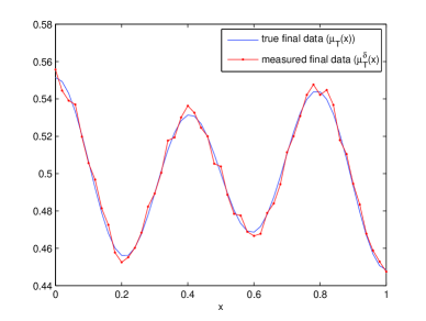
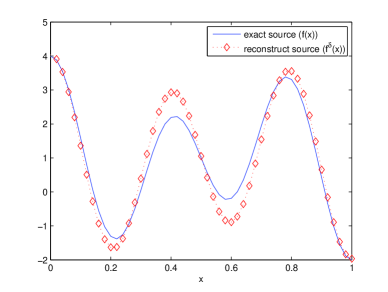
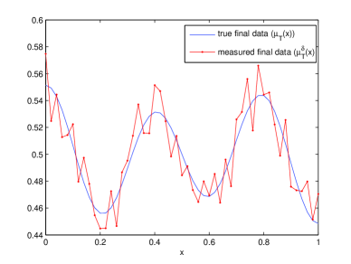
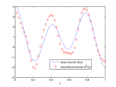
Figure 1: Comparison of convergence results. The top two with the noise level $1\%$ and $\vartheta=12$, while the bottom two with the noise level $5\%$ and $\vartheta=18$. The left are the final data and corresponding measurement error data. The other parameters are $p=1/3$, $\sigma=0.2$.

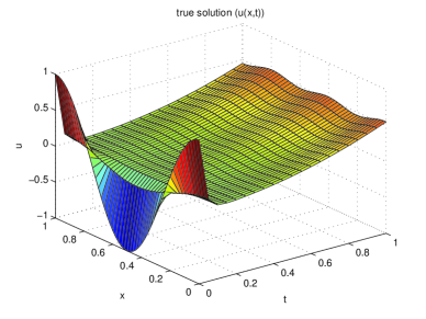
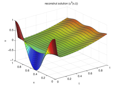
Figure 2: Comparison of true solution and reconstruct solution. The noise level is $1\%$ and $\vartheta=12$, $p=1/3$, $\sigma=0.2$.

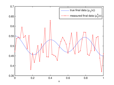
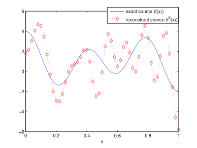
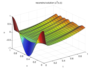
Figure 3: Convergence results with noise level $20\%$ and $\vartheta=18$, $p=1/3$, $\sigma=0.2$.

4.2 Example 2

Set $f(x)=\frac{(1-x)x}{|x-\frac{1}{2}|+\frac{1}{2}}$, $\mu_{0}(x)=0$, $h(t)=5\sin(2\pi t)+1$ and $k=1$. The true solution and the final data can be calculated by (18) (Fig. 4). Since the final data is nearly a constant function, small noise level can still produce striking different measurement data comparing with the exact data. Thus here we choose noise level with $1\%$ and $0.1\%$. Furthermore, we see that $h(t)$ does not satisfy the identically non-positive or non-negative property. However, we can still get the convergence results since $h(t)$ is not too ’bad’. Fig. 5 shows the reconstructed solution and the exact solution.

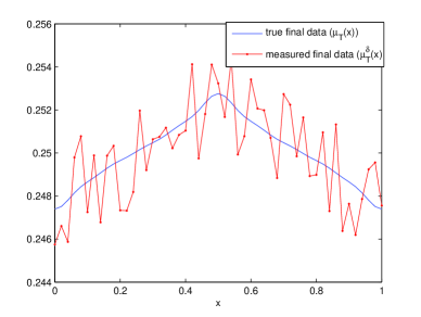
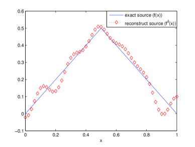
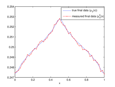
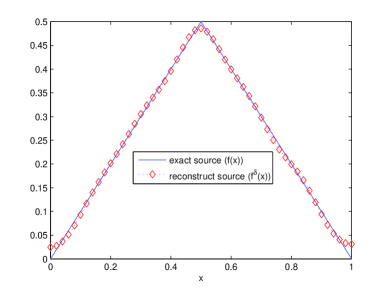
Figure 4: Comparison of convergence results. The top two with the noise level $1\%$, while the bottom two with the noise level $0.1\%$. The left are the final data and corresponding measurement error data. The other parameters are $\vartheta=12$, $p=1/3$, $\sigma=0.2$.

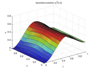
Figure 5: Comparison of true solution and reconstruct solution. The noise level is $1\%$ and $\vartheta=12$, $p=1/3$, $\sigma=0.2$.

4.3 Example 3

Set

$$f(x)=\left\{\begin{array}[]{cc}0&x<0.2\\ x&0.2\leq x\leq 0.5\\ 1-x&0.5<x\leq 0.8\\ 0&x>0.8\end{array}\right.$$

and $\mu_{0}(x)=0$, $h(t)=e^{t}+6\sin(4\pi t)+t^{2}+1$ and $k=1$. The source $f(x)$ has two discontinuous points ($x=0.2,0.8$) and one non-differentiable point ($x=0.5$). We see from Fig. 6 that the source can still be reconstructed accurately in a ’smooth’ way when the noise level is not high. Fig. 7 shows the comparison between the true solution and the reconstructed solution.

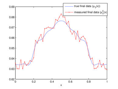
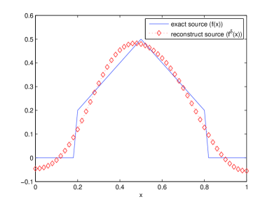
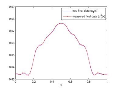
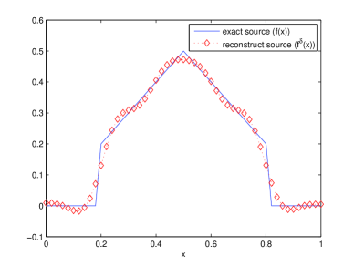
Figure 6: Comparison of convergence results. The top two with the noise level $1\%$, while the bottom two with the noise level $0.1\%$. The left are the final data and corresponding measurement error data. The other parameters are $\vartheta=12$, $p=1/3$, $\sigma=0.2$.

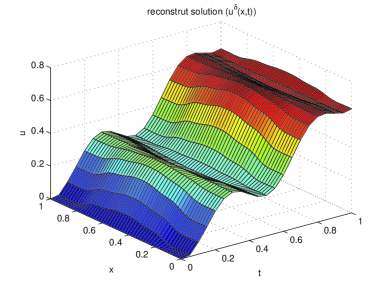
Figure 7: Comparison of true solution and reconstruct solution. The noise level is $0.1\%$ and $\vartheta=12$, $p=1/3$, $\sigma=0.2$.

5 Conclusions

In this paper, the numerical methods for reconstruction of source term in both no boundary and Neumann boundary conditions are presented. The convergence rate has been proved for both a priori and a posteriori stopping rules. More importantly, we show that the solution of the boundary conditions problem has the form of solution for the no boundary problem, which can be applied for both Neumann and Drichlet boundary conditions. The numerical experiments have shown that the frequency cut-off technique method applies well for the boundary conditions problem, although for more accurate results we may implement the iterative methods together with the a posteriori stopping rule. The numerical methods can be moved parallel to the two dimensional inverse source problem.

References

- (1) J. Bear, Dynamics of Fluids in Porous Media, Elsevier, New York, 1972.
- (2) I. Bushuyev, Global uniqueness for inverse parabolic problems with final observation, Inverse Problems, 11(1995), L11-L16.
- (3) M. Choulli, An inverse problem for a semilinear parabolic equation, Inverse Problems, 10(1994), 1123-1132.
- (4) M. Choulli, M. Yamamoto, Generic well-posedness of an inverse parabolic problem-the Hlder-space approach, Inverse Problems, 12(1996), 195-205.
- (5) J. R. Cannon, P. DuChateau, An inverse problem for an unknown source in a heat equation, J. Math. Anal. Appl., 75(1980), 465-485.
- (6) J.R. Cannon, P. Duchateau, Structural identification of an unknown source term in a heat equation, Inverse Problems, 14(1998), 535-551.
- (7) Y.J. Deng, Z.H. Liu, Iteration methods on sideways parabolic equations, Inverse Problems, 25(2009), 1-14.
- (8) Y.J. Deng, Z.H. Liu, New fast iteration for determining surface temperature and heat flux of general sideways parabolic equation, Nonlinear Analysis: Real World Applictions, 12(2011), 156-166.
- (9) H.W. Engl, M. Hanke, and A. Neubauer, Regularization of Inverse Problems, Kluwer Academic Publishers, 1996.
- (10) L. Evans, Partial Differential Equations, Providence: American Mathematical Society, 1998.
- (11) A. Hasanov, Simultaneous determination of source terms in a linear parabolic problem from the final overdetermination: Weak solution approach, J. Mathmatical Analysis and Application, 330(2007), 766-779.
- (12) M.I. Ivanchov, The inverse problem of determining the heat source power for a parabolic equation under arbitrary boundary conditions, J. Math. Sci., 88(1998), 432-436.
- (13) Andreas Kirsch, An Introduction to the Mathematical Theory of Inverse Problems, Springer-Verlag, 1996.
- (14) L. Ling, M. Yamamoto, Y. C. Hon, etc., Identification of source locations in two-dimensional heat equations, Inverse Problems, 22(2006), 1289-1305.
- (15) V.A. Morozov, On the solution of functional equations by the method of regularization, Soviet Math. Dokl., 7(1966), 414-417.
- (16) G. zkum, A. Demir, S. Erman, E. Korkmaz, and B. zgr, On the Inverse Problem of the Fractional Heat-Like Partial Differential Equations: Determination of the Source Function, Adv. in Math. Phys., vol. 2013, doi:10.1155/2013/476154.
- (17) M. Renardy, W.J. Hursa, J.A. Nohel, Mathematical Problems in Viscoelasticity, Wiley, New York, 1987.
- (18) G.M. Vainikko, A.Y. Veretennikov, Iteration Procedures in Ill-Posed Problems. Moscow, Nauka (in Russian) McCormick, S.F., 1986.
- (19) R.H.S. Winterton, Heat transfer, Oxford University Press, Oxford, 1997.
- (20) C. Zheng, G.D. Bennett, Applied Contaminant Transport Modelling: Theory and Practice, Van Nostrand Reinhold, New York, 1995.