Probabilistic picture for medium-induced jet evolution

Abstract

A high energy jet that propagates in a dense medium generates a cascade of partons that can be described as a classical branching process. A simple generating functional for the probabilities to observe a given number of gluons at a given time is derived. This is used to obtain an evolution equation for the inclusive one-gluon distribution, that takes into account the dependence upon the energy and the transverse momentum of the observed gluon. A study of the explicit transverse momentum dependence of the splitting kernel leads us to identify large corrections to the jet quenching parameter $\hat{q}$.

1 Introduction

The recent experimental results from heavy ion experiments at RHIC and LHC provide a strong motivation for improving and extending current theories of jet propagation in a dense QCD medium such as a quark-gluon plasma. Most noteworthy are those data that reveal the jet inner structure Aad:2010bu ; Chatrchyan:2011sx ; Chatrchyan:2012nia ; Aad:2012vca ; Chatrchyan:2013kwa , and in particular show that much of the energy lost in the medium is in the form of low energy quanta emitted at large angles with respect to the jet axis. Such data call for the development of new theoretical tools allowing us to explore jet quenching phenomena beyond the energy loss from the leading particle, a subject that has been thoroughly studied within the BDMPSZ framework during the last twenty years or so Baier:1996kr ; Baier:1996sk ; Baier:1998kq ; Zakharov:1996fv ; Zakharov:1997uu . Further related developments are presented in Wiedemann:2000za ; Gyulassy:2000er ; Arnold:2002ja .

In order to understand how the QCD shower gets modified as the jet traverses a dense medium, one needs to study how color coherence, and interference between subsequent emissions, are affected by the medium. These two effects play a major role in determining jet-structure in vacuum. Recent studies MehtarTani:2010ma ; MehtarTani:2011tz ; CasalderreySolana:2011rz ; MehtarTani:2011gf ; MehtarTani:2011jw ; CasalderreySolana:2012ef have shown how, in certain regimes, color coherence can be destroyed by the presence of a dense medium, and how this may lead to the suppression of angular ordering (a characteristic feature of the vacuum QCD cascade), and the enhancement of large angle emissions. In a previous paper Blaizot:2012fh we showed explicitly that the loss of color coherence occurs on a time scale comparable to that of the branching process, so that gluons that emerge from a splitting propagate independently of each other. The branching time, which is proportional to the square root of the energy of the emitted gluons, can be short for soft enough gluons, and multiple branching play an important role if the size of the medium is large enough: these multiple branching constitute the in-medium QCD cascade.

The goal of this paper is to complete the description of this cascade. It is organized as follows. In the next section we briefly recall the main results of Ref. Blaizot:2012fh concerning the properties of the medium induced gluon splitting and of transverse momentum broadening within the BDMPSZ framework. Then, in Section 3, we construct a generating functional for the probabilities to observe $n$ gluons in the cascade, at any given time. This is then used to derive the evolution equation for the inclusive one-gluon spectrum. This equation generalizes that studied in Ref. Blaizot:2013hx in that it takes into account the dependence of the distribution function on the transverse momentum of the produced gluon, as generated via collisions in the medium. (The equation studied in Blaizot:2013hx concerns only the energy distribution, that is, the integral of the one-gluon spectrum over the transverse momentum.) The kernel of this equation, however, is completely integrated over the transverse momenta and contains information on these transverse momenta only in an average way: this follows from the fact that the transverse momentum broadening acquired during the branching processes can be neglected as compared to that accumulated via collisions in the medium in between successive branchings. Thus, to the accuracy of interest, the splittings can be effectively treated as being collinear. By trying to improve the description and take into account more explicitly the transverse momentum dependence of the splitting kernel, we were led to identify large radiative corrections, which are formally infrared divergent, and are best interpreted as corrections to the transport coefficient $\hat{q}$, which is a measure of the transverse momentum square acquired by the jet parton in the medium, per unit length. This will be discussed in Section 4. In particular, we recover the double logarithmic correction to transverse momentum broadening that has been calculated recently Liou:2013qya . Technical material is gathered in three Appendices. The first one complements results obtained in Blaizot:2012fh , and gives an explicit expression for the splitting kernel in the harmonic approximation, with full dependence on transverse momenta. The contribution of the single scattering is emphasized. The second appendix is devoted to the calculation of the double logarithmic contribution to $\hat{q}$. The third appendix presents an alternative form of the generating functional that may be more suitable for Monte-Carlo calculations.

2 Basic elements

A large part of the material of this section is borrowed from Ref. Blaizot:2012fh to which we refer for more details. We consider energetic partons traversing a medium with which they exchange color and transverse momentum. This medium is modeled as a random color field, with the only non-trivial correlator (in light-cone gauge $A^{+}=0$) given by

$$\left\langle A^{-}_{a}({\bm{q}},t)A^{*-}_{b}({\bm{q}}^{\prime},t^{\prime})\right\rangle=\delta_{ab}n(t)\delta(t-t^{\prime})(2\pi)^{2}\delta^{(2)}({\bm{q}}-{\bm{q}}^{\prime})\,\gamma({\bm{q}})\;,$$ (1)

with $n$ the color charge density (which may depend on the light-cone time $t$), and we have assumed translational invariance in the transverse plane. Here, $\gamma({\bm{q}})\simeq g^{2}/{\bm{q}}^{4}$, with ${\bm{q}}$ a vector in the transverse plane, is a correlator that accounts for the elastic collisions of the energetic patrons with the medium particles. The infrared behavior of $\gamma({\bm{q}})$ is controlled by the Debye screening mass $m_{D}$, which is the typical momentum exchanged in a collision with medium particles.

Consider now the process in which a gluon is created inside the medium with momentum $\vec{p}_{0}\equiv(p_{0}^{+},{\bm{p}}_{0})$ at time $t_{0}$. In practice, we shall eventually chose $\bm{p}_{0}=\bm{0}$, that is, we shall use the direction of motion of the leading particle to define the longitudinal direction with respect to which one measures polar angles and transverse momenta. For $t>t_{0}$, the gluon propagates through the medium and interacts with the latter. In leading order, that is, in the absence of splitting, all what happens to it is that it receives transverse momentum kicks in colliding with the medium constituents. When it emerges from the medium, at time $t_{L}$, its momentum is $\vec{k}=(k^{+},{\bm{k}})$. Let us denote by $P_{1}(\vec{k};t_{L},t_{0}){\rm d}\Omega_{k}$ the probability to observe the gluon at time $t_{L}$ with its momentum in the phase-space element ${\rm d}\Omega_{k}$, given that, at time $t_{0}$ its momentum is in the phase-space element ${\rm d}\Omega_{p_{0}}$. Here, $d\Omega_{k}\equiv(2\pi)^{-3}{\rm d}^{2}{\bm{k}}\,dk^{+}/2k^{+}$ is the invariant phase-space element. The probability $P_{1}$ contains, quite generally, a delta function that expresses the conservation of the + component of the momentum (that follows from the fact that the medium is assumed homogeneous in $x^{-}$), and it is convenient to write it as

$$P_{1}(\vec{k};t_{L},t_{0})=2p_{0}^{+}\,2\pi\delta(k^{+}-p_{0}^{+}){\cal P}_{1}({\bm{k}};t_{L},t_{0}).$$ (2)

In leading order, ${\cal P}_{1}({\bm{k}};t_{L},t_{0})$ can be identified with the probability for the gluon to acquire a transverse momentum ${\bm{k}}-{\bm{p}}_{0}$ from the medium during its propagation from time $t_{0}$ to time $t_{L}$, a quantity that we shall denote simply by ${\cal P}({\bm{k}}-{\bm{p}}_{0};t_{L},t_{0})$ throughout the paper. This probability ${\cal P}$ is well known, and it can be written as

$${\cal P}({\bm{k}}-{\bm{p}}_{0};t_{L},t_{0})=\int{\rm d}^{2}{\bm{r}}\exp\left[-i({\bm{k}}-{\bm{p}}_{0})\cdot{\bm{r}}-\frac{N_{c}}{2}\int_{t_{0}}^{t_{L}}dt\,n(t)\sigma({\bm{r}})\right],$$ (3)

with $\sigma({\bm{r}})$ the ‘dipole cross section’

$$\sigma({\bm{r}})=2g^{2}\int\frac{{\rm d}^{2}{\bm{q}}}{(2\pi)^{2}}\left(1-{\rm e}^{i{\bm{q}}\cdot{\bm{r}}}\right)\,\gamma({\bm{q}}).$$ (4)

Note that $\sigma(r\to 0)\to 0$, a property commonly referred to as color transparency; this ensures in particular that the probability ${\cal P}$ is properly normalized: $\int_{\bm{k}}{\cal P}({\bm{k}}-{\bm{p}}_{0};t,t_{0})\,=\,1$. The Fourier transform of the dipole cross section reads

$$\sigma({\bm{l}})=\int{\rm d}{\bm{r}}\,{\rm e}^{-i{\bm{l}}\cdot{\bm{r}}}\sigma({\bm{r}})=-2g^{2}\left[\gamma({\bm{l}})-(2\pi)^{2}\delta({\bm{l}})\int_{{\bm{q}}}\gamma({\bm{q}})\right],$$ (5)

and it obeys the properties (to be used later)

$$\int_{\bm{l}}\sigma({\bm{l}})=0=\int_{\bm{l}}{\bm{l}}\,\sigma({\bm{l}}).$$ (6)

In the equations above, we introduced a shorthand notation for the transverse momentum integrations: $\int_{\bm{q}}\equiv\int{\rm d}^{2}{\bm{q}}/(2\pi)^{2}$. This will be used throughout the paper.

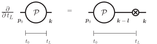
Figure 1: Diagrammatic representation of the evolution of the broadening probability (7).

By taking the derivative of Eq. (3) with respect to $t_{L}$ (and setting $t_{L}=t$), one easily obtains

$$\frac{\partial}{\partial t}{\cal P}({\bm{k}}-{\bm{p}}_{0};t,t_{0})=\int_{\bm{l}}\,{\cal C}({\bm{l}},t)\,{\cal P}({\bm{k}}-{\bm{p}}_{0}-{\bm{l}};t,t_{0})\,,$$ (7)

with

$${\cal C}({\bm{l}},t)\equiv 4\pi\alpha_{s}N_{c}n(t)\left[\gamma({\bm{l}})-(2\pi)^{2}\delta^{(2)}({\bm{l}})\int_{\bm{q}}\gamma({\bm{q}})\right]=-\frac{1}{2}N_{c}n(t)\sigma({\bm{l}}).$$ (8)

This equation can be simplified by taking into account the fact that the typical momentum transferred in one collision is $|{\bm{l}}|\sim m_{D}$ and is much smaller than the transverse momentum $|{\bm{k}}|\sim Q_{s}\equiv\sqrt{\hat{q}L}$ acquired by the gluon during its propagation over a distance comparable to $L$, the size of the medium. Under such circumstances, Eq. (7) can be reduced to the following Fokker-Planck equation:

$$\frac{\partial}{\partial t}{\cal P}({\bm{k}}-{\bm{p}}_{0};t,t_{0})=\frac{1}{4}\frac{\partial^{2}}{\partial{\bm{k}}^{2}}\left[\hat{q}(t,{\bm{k}}^{2})\,{\cal P}({\bm{k}}-{\bm{p}}_{0};t,t_{0})\right]\,,$$ (9)

with the jet quenching parameter $\hat{q}(t,{\bm{k}}^{2})$, playing the role of a diffusion coefficient, given by

$$\hat{q}(t,{\bm{k}}^{2})=-{N_{c}n(t)}\int_{{\bm{l}}}{\bm{l}}^{2}\sigma({\bm{l}})=g^{2}N_{c}n(t)\int_{\bm{l}}{\bm{l}}^{2}\gamma({\bm{l}})\approx 4\pi\alpha_{s}^{2}N_{c}n(t)\ln\frac{{\bm{k}}^{2}}{m_{D}^{2}}.$$ (10)

The above integral, which determines the value of $\hat{q}$, is logarithmically divergent. It is naturally cut-off at its lower end by the Debye mass, and at its upper end by the momentum scale ${\bm{k}}$ at which ${\cal P}$ is evaluated. Note that in deriving Eq. (9) attention has been paid to this momentum dependence of $\hat{q}$. It can be verified in particular that, as written, the right hand side of the equation vanishes upon integration over ${\bm{k}}$, as it should.

An alternative interpretation of $\hat{q}$ is obtained by expanding the dipole cross section (4) to quadratic order in the dipole size. This yields

$$N_{c}n(t)\sigma({\bm{r}})\simeq\frac{1}{2}\,\hat{q}(t,1/r^{2})\,{\bm{r}}^{2},$$ (11)

where the inverse of the dipole size $r$ plays the role of ultraviolet cut-off. This expression, when used with a constant $\hat{q}$ (i.e., ignoring the dependence of $\hat{q}$ on the dipole size), is referred to as the ‘harmonic approximation’. Within this approximation, the diffusion equation (9) is easily solved. Assuming $n$, and hence $\hat{q}$, to be independent of $t$ for simplicity, one gets

$${\cal P}({\bm{k}}-{\bm{p}}_{0};t,t_{0})=\frac{4\pi}{\hat{q}(t-t_{0})}{\rm e}^{-\frac{({\bm{k}}-{\bm{p}}_{0})^{2}}{\hat{q}(t-t_{0})}}.$$ (12)

The diffusion picture is valid in the regime dominated by multiple scattering, in which a large transverse momentum is achieved by the addition of many small momentum transfers over the propagation time $\Delta t=t-t_{0}$. This regime holds for $k^{2}\lesssim\hat{q}\Delta t$. Larger transverse momenta can be achieved, over comparable time scales, through a single hard scattering. The corresponding expression for ${\cal P}$ is not given by the diffusion equation, but rather by using the first iteration of Eq. (7) or, equivalently, by expanding the exponential in Eq. (3) to linear order in $\sigma$. Either way, one finds that in the regime where $k^{2}\gg\hat{q}(t_{L}-t_{0})$:

$${\cal P}({\bm{k}};t_{L},t_{0})\simeq\,\frac{16\,\pi^{2}\,\alpha_{s}^{2}\,N_{c}}{{\bm{k}}^{4}}\,\int_{t_{0}}^{t_{L}}dt\,n(t)\,.$$ (13)

Let us now turn to the process of in-medium gluon branching which was studied in detail in Blaizot:2012fh . A major assumption in that calculation is that the branching time $\tau_{{}_{\rm br}}\simeq\sqrt{\omega_{0}/\hat{q}_{0}}$ is much shorter than the time $t_{L}-t_{0}$ spent by the partons in the medium, or equivalently $\omega_{0}\lesssim\omega_{c}=\hat{q}_{0}t_{L}^{2}$, where $\omega_{c}$ is the maximum energy that can be taken away by an offspring gluon, i.e., $\tau_{{}_{\rm br}}(\omega_{c})=t_{L}-t_{0}$. (We have set $\omega_{0}\equiv z(1-z)p_{0}^{+}$, and $\hat{q}_{0}\equiv\hat{q}f(z)$ with $f(z)=1-z(1-z)$ ; see also Appendix A and Eq. (16) below.)

Let $P_{2}(\vec{k}_{a},\vec{k}_{b};t_{L},t_{0}){\rm d}\Omega_{k_{a}}{\rm d}\Omega_{k_{b}}$ be the probability to observe two gluons at time $t_{L}$ in the phase space elements ${\rm d}\Omega_{k_{a}}$ and ${\rm d}\Omega_{k_{b}}$, respectively, given that one gluon was present in the phase-space element ${\rm d}\Omega_{p_{0}}$ at time $t_{0}$. Similarly to what we did for $P_{1}$ in Eq. (2), we separate the delta function that expresses the conservation of the + momentum and write

$$P_{2}(\vec{k}_{a},\vec{k}_{b};t_{L},t_{0}) = 2p_{0}^{+}\,2\pi\delta(k_{a}^{+}+k_{b}^{+}-p_{0}^{+})\,{\cal P}_{2}({\bm{k}}_{a},{\bm{k}}_{b},z;t_{L},t_{0}).$$ (14)

In Appendix A, it is recalled that when one drops all possible terms that are suppressed by at least one power of $\tau_{\rm br}/L$, one ends up with a simple formula for ${\cal P}_{2}$:

$${\cal P}_{2}({\bm{k}}_{a},{\bm{k}}_{b},z;t_{L},t_{0}) =2g^{2}z(1-z)\int_{t_{0}}^{t_{L}}\,{\rm d}t\,{\cal K}(z,p_{0}^{+};t)$$

$$\times\int_{{\bm{q}}}\;{\cal P}({\bm{k}}_{a}-z{\bm{q}};t_{L},t)\,{\cal P}({\bm{k}}_{b}-(1-z){\bm{q}};t_{L},t){\cal P}({\bm{q}}-{\bm{p}}_{0};t,t_{0}),$$ (15)

where ${\cal K}(z,p_{0}^{+};t)$ is given by

$${\cal K}(z,p_{0}^{+};t)=\frac{P_{gg}(z)}{2\pi}\sqrt{\frac{\hat{q}f(z)}{z(1-z)p_{0}^{+}}}=\frac{P_{gg}(z)}{2\pi}\sqrt{\frac{\hat{q}_{0}}{\omega_{0}}},\qquad f(z)=1-z+z^{2},$$ (16)

with

$$P_{gg}(z)=N_{c}\,\frac{[1-z(1-z)]^{2}}{z(1-z)}=N_{c}\frac{[f(z)]^{2}}{z(1-z)}$$ (17)

the leading–order Altarelli–Parisi gluon splitting function Altarelli:1977zs . We may interpret the integrand of Eq. (2) as a product of probabilities: the probability ${\cal P}({\bm{q}}-{\bm{p}}_{0};t,t_{0})$ for the initial gluon to acquire transverse momentum ${\bm{q}}-{\bm{p}}_{0}$ in time $t-t_{0}$, the probability ${\cal K}(z,p_{0}^{+};t){\rm d}t$ for the gluon to split between times $t$ and $t+{\rm d}t$, into two gluons with energy fractions $z$ and $1-z$, and the probabilities for the offspring gluons to evolve to momenta ${\bm{k}}_{a}$ and ${\bm{k}}_{b}$, respectively ${\cal P}({\bm{k}}_{a}-{\bm{p}};t_{L},t)$ and ${\cal P}({\bm{k}}_{b}-{\bm{q}}+{\bm{p}};t_{L},t)$.

Note that the splitting described by Eq. (2) is collinear : just after the splitting, the daughter gluons carries equal fractions, $z$ and respectively $1-z$, of both the longitudinal momentum $p_{0}^{+}$ and the transverse momentum ${\bm{q}}$ of their parent gluon. This is a consequence of the leading order approximation in which we ignore, in the factors ${\cal P}$, the small contribution to momentum broadening that may occur during the branching process (such small contributions are taken into account in an average way in the kernel). As a result, in the leading order approximation, transverse momentum is gained only in between the splittings, through momentum space diffusion.

Eq. (2) will be at the basis of the classical branching process to be constructed in the next section. However, in the last section of this paper we shall examine a more complete version of the splitting kernel, which keeps track of the transverse momentum that is acquired during the branching process. This is obtained by relaxing some of the approximations leading to Eq. (2), and involves corrections, a priori small since of order $\tau_{{}_{\rm br}}/L$, but which happen to be amplified by logarithmic divergences. As we shall see, these corrections are best interpreted as corrections to $\hat{q}$, or equivalently as corrections to the interaction between the partons of the cascade and the medium particles.

3 Generating functional and inclusive one-gluon distribution

In this section, we introduce the generating functional that describes the in-medium gluon cascade, under the assumption that successive branchings can be treated as independent, in line with the results of Ref. Blaizot:2012fh . The generating functional follows simply from iterating the elementary $1\to 2$ splitting process whose properties are recalled in the previous section. From the generating functional, we derive the equation for the inclusive one-gluon distribution function and we analyze some of its properties.

3.1 Generalities

We consider an in-medium parton shower initiated at (light-cone) time $t_{0}$ by a ‘leading parton’ with 3–momentum ${\vec{p}}_{0}\equiv(p^{+}_{0},\bm{p}_{0})$. The generating functional ${\cal Z}_{p_{0}}\,[t,t_{0}|u]$, with $t_{0}\leq t\leq t_{L}$, is defined as

$${\cal Z}_{p_{0}}[t,t_{0}|u]=\sum_{n=1}^{\infty}\frac{1}{n!}\int\left(\prod_{i=1}^{n}\,{\rm d}\Omega_{i}\right)\,P_{n}({\vec{k}}_{1},\cdots,{\vec{k}}_{n};t,t_{0})\,u({\vec{k}}_{1})\cdots u({\vec{k}}_{n})\,$$ (18)

where $u\equiv u({\vec{k}})$ is a generic function of ${\vec{k}}$ and $P_{n}({\vec{k}}_{1},\cdots,{\vec{k}}_{n};t,t_{0})$ is the probability density to find at time $t$ exactly $n$ gluons with momenta ${\vec{k}}_{1},\cdots,{\vec{k}}_{n}$ such that $k^{+}_{1}+\cdots+k^{+}_{n}=p_{0}^{+}$ (recall that the + component of the momentum is conserved during the branchings). The function $P_{n}({\vec{k}}_{1},\cdots,{\vec{k}}_{n};t,t_{0})$ is totally symmetric under the permutations of the $n$ variables ${\vec{k}}_{1},\cdots,{\vec{k}}_{n}$. Leading order expressions for the probabilities $P_{1}$ and $P_{2}$ have been given in the previous section. Note that, ${\cal Z}_{p_{0}}[t,t_{0}|u=1]=1$, which reflects the normalization of the probabilities, while obviously ${\cal Z}_{p_{0}}[t,t_{0}|u=0]=0$.

By taking the $n$th functional derivative of ${\cal Z}_{p_{0}}[t,t_{0}|u]$ evaluated at $u=0$, one recovers $P_{n}({\vec{k}}_{1},\cdots,{\vec{k}}_{n};t,t_{0})$:

$$P_{n}({\vec{k}}_{1},\cdots,{\vec{k}}_{n};t,t_{0})=\left.\left[\prod_{i=1}^{n}\,(2\pi)^{3}\,2k^{+}_{i}\,\frac{\delta}{\delta u({\vec{k}}_{i})}\right]{\cal Z}_{p_{0}}[t,t_{0}|u]\right|_{u=0}\,,$$ (19)

with the usual definition

$$\frac{\delta u({\vec{k}})}{\delta u({\vec{q}})}=\delta^{(3)}({\vec{k}}-{\vec{q}})\equiv\delta(k^{+}-q^{+})\,\delta^{(2)}({\bm{k}}-{\bm{q}})\,.$$ (20)

We shall be mostly concerned with inclusive probabilities, that is by the probabilities to observe at time $t$, $n$ gluons with specified momenta, irrespective of whether other gluons are produced or not. Such probabilities are obtained by taking the $n$-th functional derivative of ${\cal Z}_{p_{0}}[t,t_{0}|u]$ and then letting $u=1$.

3.2 Evolution equations for the generating functional

Two formulations can be considered for the evolution of the generating functional. We consider in this section the ‘forward’, formulation, where an additional splitting is allowed to occur at the latest time $t$ of the cascade development. In Appendix C, another formulation is presented, where one focuses instead on a splitting taking place at the beginning of the cascade. Both formulations are equivalent but lead to different equations (see e.g. Ref. Cvitanovic:1980ru for a general discussion).

Let us then consider the initial state of the cascade, where a single gluon is present at time $t=t_{0}$. For $t=t_{0}$, all probabilities vanish except $P_{1}({\vec{k}};t_{0},t_{0})=2k^{+}(2\pi)^{3}\delta(\vec{k}-\vec{p}_{0})$, so that the generating functional reduces to

$${\cal Z}_{p_{0}}[t_{0},t_{0}|u]\,=\,u({\vec{p}}_{0})\,.$$ (21)

During the infinitesimal time step $t_{0}\to t_{0}+{\rm d}t$, two physical effects can occur: momentum broadening and splitting. Only the variations with time of $P_{1}$ and $P_{2}$ contribute: $P_{2}$ changes because a splitting can occur during the time ${\rm d}t$; $P_{1}$ changes for two reasons: first the collisions change the transverse momentum, second, probability conservation forces $P_{1}$ to decrease as $P_{2}$ increases. Thus, at time $t_{0}+{\rm d}t$, the generating functional reads

$${\cal Z}_{p_{0}}[t_{0}+{\rm d}t,t_{0}|u] = \int{\rm d}\Omega_{k}\,P_{1}(\vec{k};t_{0}+{\rm d}t,t_{0})\,u(\vec{k})$$ (22)

$$+ \frac{1}{2}\int{\rm d}\Omega_{k_{1}}{\rm d}\Omega_{k_{2}}\,P_{2}({\vec{k}}_{1},{\vec{k}}_{2};{\vec{p}}\,;t_{0}+{\rm d}t,t_{0})\,u({\vec{k}}_{1})u({\vec{k}}_{2}),$$

where $P_{1}$ contains, besides the leading order contribution, a contribution of order $\alpha_{s}$, for the reason just mentioned.

The leading order variation of $P_{1}$, which corresponds to momentum broadening, is easily deduced from Eq. (7). The order $\alpha_{s}$ correction will be inferred from the conservation of probability. For $P_{2}$ we use the definition (14) to write

$$\frac{1}{2}\int{\rm d}\Omega_{1}{\rm d}\Omega_{2}\,P_{2}(\vec{k}_{1},\vec{k}_{2};t,t_{0})\,u(\vec{k}_{1})u(\vec{k}_{2})$$

$$=\frac{1}{4\pi}\int_{0}^{1}\frac{{\rm d}z}{2z(1-z)}\int_{{\bm{k}}_{1},{\bm{k}}_{2}}\,{\cal P}_{2}({\bm{k}}_{1},{\bm{k}}_{2},z;t,t_{0})\;u(zp_{0}^{+},{\bm{k}}_{1})\,u((1-z)p_{0}^{+},{\bm{k}}_{2}),$$ (23)

where we have used

$$k_{1}^{+}=zp_{0}^{+},\quad k_{2}^{+}=(1-z)p_{0}^{+},\quad{\rm d}\Omega_{1}{\rm d}\Omega_{2}=\frac{1}{(2\pi)^{2}}\frac{{\rm d}z{\rm d}p_{0}^{+}}{4z(1-z)p_{0}^{+}}.$$ (24)

Next, by taking a derivative w.r.t. $t_{L}$ on (2), and relabeling $t_{L}\to t$, ${\bm{k}}_{a}\to{\bm{k}}_{1}$, and ${\bm{k}}_{b}\to k_{2}$, one deduces

$$\partial_{t}{\cal P}_{2}({\bm{k}}_{1},{\bm{k}}_{2},z;t,t_{0})= 2g^{2}z(1-z){\cal K}(z,p_{0}^{+};t)$$

$$\times\int_{{\bm{q}}}(2\pi)^{4}\delta^{(2)}({\bm{k}}_{1}-z{\bm{q}})\delta^{(2)}({\bm{k}}_{2}-(1-z){\bm{q}}){\cal P}({\bm{q}}-{\bm{p}}_{0};t,t_{0}),$$ (25)

and hence [recall that ${\cal P}({\bm{q}}-{\bm{p}}_{0};t_{0},t_{0})=(2\pi)^{2}\delta^{(2)}({\bm{q}}-{\bm{p}}_{0})$]

$${\cal P}_{2}({\bm{k}}_{a},{\bm{k}}_{b},z;t_{0}+{\rm d}t,t_{0})=2g^{2}z(1-z)\,{\cal K}(z,p_{0}^{+};t_{0}){\rm d}t\ (2\pi)^{4}\delta^{(2)}({\bm{k}}_{1}-z{\bm{p}}_{0})\delta^{(2)}({\bm{k}}_{2}-(1-z){\bm{p}}_{0}).$$ (26)

Combining these results, on can rewrite ${\cal Z}_{p_{0}}[t_{0}+{\rm d}t,t_{0}|u]$ as follows

$$\left.\frac{\partial}{\partial t}{\cal Z}_{p_{0}}[t,t_{0}|u]\right|_{t=t_{0}}= \int_{{\bm{l}}}\,{\cal C}({\bm{l}},t_{0})\,u(p_{0}^{+},{\bm{p}}_{0}+{\bm{l}})$$

$$+\alpha_{s}\int_{0}^{1}{\rm d}z\,{\cal K}(z,p_{0}^{+};t)\Big{[}u(zp_{0}^{+},z{\bm{p}}_{0})\,u((1-z)p_{0}^{+},(1-z){\bm{p}}_{0})-u(\vec{p}_{0})\Big{]}.$$ (27)

Note that the last term, proportional to $u(\vec{p}_{0})$ is here to ensure that the probability is conserved during the evolution: if one sets $u=1$, then all terms in the right-hand-side of Eq. (3.2) vanish (recall that $\int_{\bm{l}}{\cal C}({\bm{l}})=0$).

Equation (3.2) is easily extended to a full evolution equation for the generating functional This evolution equation for ${\cal Z}$ reads

$$\frac{\partial}{\partial t_{L}}{\cal Z}_{p_{0}}[t_{L},t_{0}|u]-\int\frac{{\rm d}q^{+}}{2\pi}\int_{{\bm{q}}}\int_{{\bm{l}}}u(q^{+},{\bm{q}}+{\bm{l}})\,{\cal C}({\bm{l}},t_{L})\,\frac{\delta}{\delta u(\vec{q})}\,{\cal Z}_{p_{0}}[t_{L},t_{0}|u]$$

$$= \alpha_{s}\int_{0}^{1}{\rm d}z\,\int\frac{{\rm d}q^{+}}{2\pi}\int_{{\bm{q}}}{\cal K}(z,q^{+};t)\Big{[}u(zq^{+},z{\bm{q}})\,u((1-z)q^{+},(1-z){\bm{q}})-u(\vec{q})\Big{]}\frac{\delta}{\delta u(\vec{q})}{\cal Z}_{p_{0}}[t_{L}|u]\,.$$

This formula has a simple interpretation. The effect of the functional derivative $\delta/\delta u({\vec{q}})$ is to select a gluon with momentum ${\vec{q}}$ from the gluon cascade at time $t_{L}$. Then one calculates the evolution of this particular gluon by repeating the infinitesimal time step discussed before. The second term in the first line accounts for the collision of the gluon with the medium which, at time $t_{L}$, turns its momentum ${\bm{q}}$ into ${\bm{q}}+{\bm{l}}$. The second line contains the probability for this gluon to split (via a collinear splitting), or not, in the time step $t_{L}\to t_{L}+{\rm d}t_{L}$. In Appendix C, an equivalent equation is provided (cf. Eq. (86)), in which the generating functional is differentiated with respect to $t_{0}$.

At this point, it is worth recalling that the equations above are somewhat formal since the integrals over the spliting fraction $z$ develop endpoint singularities at $z=0$ and $z=1$. To see that more precisely, let us consider the evolution equation for the probability ${\cal P}_{1}({\bm{k}};t_{L},t_{0})$. By using the definition (19) together with the evolution equation (3.2), one easily finds

$$\frac{\partial}{\partial t_{L}}{\cal P}_{1}({\bm{k}};t_{L},t_{0})-\int_{{\bm{l}}}{\cal C}({\bm{l}},t_{L})\,{\cal P}_{1}({\bm{k}}-{\bm{l}};t_{L},t_{0})=-\alpha_{s}\int_{0}^{1}{\rm d}z\,{\cal K}(z,p^{+}_{0};t_{L})\,{\cal P}_{1}({\bm{k}};t_{L},t_{0})\,,$$ (29)

where the r.h.s. originates from the ‘loss’ term in Eq. (3.2) and describes the reduction of the one-gluon probability due to branching. This equation is easily solved by writing

$${\cal P}_{1}({\bm{k}};t_{L},t_{0})\,=\, \Delta(p^{+}_{0};t_{L},t_{0})\,{\cal P}({\bm{k}}-{\bm{p}}_{0};t_{L},t_{0}).$$ (30)

One then easily finds

$$\Delta(p^{+}_{0};t_{L},t_{0})\,=\, \exp\left[-\alpha_{s}\int_{t_{0}}^{t_{L}}{\rm d}t\int_{0}^{1}{\rm d}z\,{\cal K}(z,p^{+}_{0};t)\right].$$ (31)

The physical meaning of Eq. (30) is transparent: ${\cal P}_{1}({\bm{k}};t_{L},t_{0})$ appears as the product of the probability ${\cal P}({\bm{k}}-{\bm{p}}_{0};t_{L},t_{0})$ for the initial gluon (with momentum $\vec{p}_{0}$) to acquire transverse momentum ${\bm{k}}-{\bm{p}}_{0}$ via collision with the medium, multiplied by the ‘survival probability’ $\Delta(p^{+}_{0};t_{L},t_{0})$ (aka the ‘Sudakov factor’), that is the probability for this gluon not to branch between $t_{0}$ and $t_{L}$. As it stands, this survival probability vanishes because of the endpoint singularities of the kernel ${\cal K}(z,p^{+}_{0};t)$ at $z=0$ and $z=1$. A cut-off needs to be introduced, which defines the ‘resolution’, i.e., the energy below which gluons cannot be resolved anymore. The following identities ($\epsilon\to 0$), that result from the symmetry of the kernel in the substitution $z\to 1-z$,

$$\int_{\epsilon}^{1-\epsilon}{\rm d}z\,{\cal K}(z)\,=\,2\int_{0}^{1-\epsilon}{\rm d}z\,z\,{\cal K}(z)\,=\,2\int_{\epsilon}^{1}{\rm d}z\,(1-z)\,{\cal K}(z)\,,$$ (32)

allow us to concentrate on one of the two endpoint singularities, say that at $z=0$. One then easily estimates (with $\Delta t=t_{L}-t_{0}$)

$$\Delta(\epsilon p^{+}_{0};\Delta t)\simeq\,\exp\left[-2\bar{\alpha}\Delta t\sqrt{\frac{\hat{q}}{\epsilon p^{+}_{0}}}\,\right],$$ (33)

where $\bar{\alpha}\equiv\alpha_{s}N_{c}/\pi$. It follows in particular that the typical time between two successive branchings (the value of $\Delta t$ for which the exponent becomes of order one) is given by

$$\Delta t_{\rm rad}(\epsilon p^{+})\,\simeq\,\frac{1}{2\bar{\alpha}}\,\sqrt{\frac{\epsilon p^{+}}{\hat{q}}}\,\sim\,\frac{1}{\bar{\alpha}}\,\tau_{{}_{\rm br}}(\epsilon p^{+})\,,$$ (34)

for a gluon within the cascade with generic energy $p^{+}$. In order for successive branchings to proceed independently from each other, we need $\Delta t_{\rm rad}$ to be significantly larger than the duration $\tau_{{}_{\rm br}}(p^{+})$ of the branching giving birth to the $p^{+}$ gluon, which implies $\epsilon>\bar{\alpha}^{2}$. Such a cut–off must be included to give a meaning to the generating functional. Note however that physical (inclusive) distributions remain finite in the limit $\epsilon\to 0$, as we shall shortly verify, hence they are only weakly sensitive to the precise value of this cutoff, so long as it is small enough.

3.3 Evolution equation for the one-gluon distribution

We turn now to a specific study of the inclusive one-gluon distribution. To simplify the notation, we shall omit the explicit dependence on the initial momentum ${\vec{p}}_{0}\equiv(p^{+}_{0},\bm{0})$, as well as on $t_{0}$, and denote the gluon distribution simply by $D(x,{\bm{k}},t)$, with $x=k^{+}/p^{+}_{0}$. We shall also assume from now on that the density $n$ is independent of time, and therefore so is ${\cal K}$.

The inclusive one-gluon distribution is given by

$$D(x,{\bm{k}},t)=k^{+}\frac{{\rm d}N}{{\rm d}k^{+}{\rm d}^{2}{\bm{k}}} \equiv k^{+}\left\langle\sum_{n=1}^{\infty}\sum_{j=1}^{n}\delta^{(3)}({\vec{k}}_{j}-{\vec{k}})\right\rangle$$ (35)

$$= \frac{1}{2(2\pi)^{3}}\left\{P_{1}(\vec{k};t,t_{0})+\sum_{n=2}^{\infty}\frac{1}{n!}\int\prod_{i=1}^{n-1}\,{\rm d}\Omega_{i}\,n\,P_{n}({\vec{k}},{\vec{k}}_{1},\cdots,{\vec{k}}_{n-1};t,t_{0})\right\}$$

$$= \left.k^{+}\frac{\delta{\cal Z}_{p_{0}}[t,t_{0}|u]}{\delta u({\vec{k}})}\right|_{u=1}\,.$$

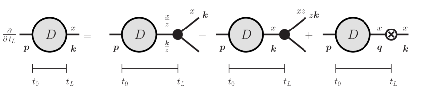
Figure 2: Diagrammatic representation of the forward evolution for the inclusive gluon distribution.

According to this formula, the evolution equation obeyed by $D(x,{\bm{k}},t)$ can be obtained by taking a functional derivative $\delta/\delta u({\vec{k}})$ of Eq. (3.2), and then setting $u=1$ (note that only the explicit factors of $u$ in Eq. (3.2) contribute in this operation). We thus find

$$\frac{\partial}{\partial t}D(x,{\bm{k}},t) =\int_{{\bm{l}}}\,{\cal C}({\bm{l}},t)D\left(x,{\bm{k}}-{\bm{l}},t\right)$$

$$+\alpha_{s}\int_{0}^{1}{\rm d}z\bigg{[}\frac{2}{z^{2}}{\cal K}\left(z,\frac{x}{z}p^{+}_{0};t\right)D\left(\frac{x}{z},\frac{{\bm{k}}}{z},t\right)-{\cal K}\left(z,xp^{+}_{0};t\right)D\left(x,{\bm{k}},t\right)\bigg{]}.$$ (36)

This equation, which represents an important result of this paper, is illustrated in Fig. 2. The first term in its r.h.s. describes transverse momentum broadening via medium rescattering in between successive branchings, and leads to diffusion in momentum space. The two terms within the square brackets in the second line of Eq. (3.3) can be viewed respectively as a ‘gain term’ and a ‘loss term’ associated with one branching. The ‘gain term’ describes the production of a new gluon with energy fraction $x$ and transverse momentum ${\bm{k}}$ via the decay of an ancestor gluon having energy fraction $x^{\prime}=x/z>x$ and transverse momentum ${\bm{k}}/z$. (Note that the condition $x<x^{\prime}<1$ implies $1>z>x$ for the respective integral over $z$.) The ‘loss term’ describes the disappearance of a gluon with energy fraction $x$ via the decay $(x,{\bm{k}})\to(zx,z{\bm{k}})\,((1-z)x,(1-z){\bm{k}})$, with $0<z<1$. Equation (3.3) thus describes the interplay between collinear splittings (cf. Eq. (2)) and diffusion in momentum space in the development of the in-medium cascade.

3.4 Energy distribution

By integrating Eq. (3.3) over the transverse momentum ${\bm{k}}$, one finds a simplified equation describing the evolution of the energy distribution alone:

$$\frac{\partial}{\partial t}D(x,t) =\alpha_{s}\int_{0}^{1}{\rm d}z\Big{[}2{\cal K}\left(z,\frac{x}{z}p^{+}_{0},t\right)D\left(\frac{x}{z},t\right)-{\cal K}\left(z,xp^{+}_{0},t\right)D\left(x,t\right)\Big{]},$$ (37)

where we have set $D(x,t)\equiv\int_{\bm{k}}D(x,{\bm{k}},t)$. Since the kernel is independent of time, the gluon distribution depends upon $t$ and $t_{0}$ only via their difference $t-t_{0}$ and it is convenient to rescale the time variable and the emission kernel in such a way as to construct dimensionless quantities. Namely, we define

$$\tau\equiv\,\frac{\alpha_{s}N_{c}}{\pi}\sqrt{\frac{\hat{q}}{p^{+}_{0}}}\,(t-t_{0})\,,\qquad\hat{\cal K}(z)\equiv\frac{2\pi}{N_{c}}\sqrt{\frac{p^{+}_{0}}{\hat{q}}}\,{\cal K}(z,p^{+}_{0})\,=\,\frac{[1-z(1-z)]^{5/2}}{[z(1-z)]^{3/2}}\,.$$ (38)

Using also the property (cf. Eq. (16))

$${\cal K}\left(z,\frac{x}{z}p^{+}_{0}\right)\,=\,\sqrt{\frac{z}{x}}\,{\cal K}(z,p^{+}_{0}),$$ (39)

as well as the identities Eq. (32), one can put the evolution equation (37) in the form

$$\frac{\partial}{\partial\tau}D(x,\tau)=\int{\rm d}z\,\hat{\cal K}(z)\left[\sqrt{\frac{z}{x}}D\left(\frac{x}{z},\tau\right)-\frac{z}{\sqrt{x}}D(x,\tau)\right],$$ (40)

which is the equation that has been studied in Ref. Blaizot:2013hx .

Note that the singularities of the kernel $\hat{\cal K}(z)$ at $z=0$ and $z=1$ are here harmless, since they exactly cancel: the integral over $z$ in the ‘gain’ term is restricted to $z>x$, while that in the ‘loss’ term involves an additional factor of $z$, which ensures convergence as $z\to 0$. When $z\to 1$, the ‘gain’ and ‘loss’ terms would separately be singular, yet the respective divergences cancel in their sum, provided the spectrum $D(x,\tau)$ is a regular function of $x$ for $x<1$. Accordingly, Eq. (40) is well defined as written, and the same applies to Eq. (3.3).

4 Radiative corrections to $\hat{q}$

As recalled in the Appendix A, several approximations are involved in the derivation of the splitting kernel. Among those are approximations in which one ignores small momenta in the propagators ${\cal P}$, thereby allowing us to integrate the kernel over those particular momenta. Such approximations are in line with the leading order of our approximation scheme. However, in integrating the kernel over the various transverse momenta on which it may depend, one eliminates potentially interesting physics: we have seen in particular that in the leading order of our approximation scheme, the gluon splitting is strictly collinear, with all transverse momenta arising from collisions with medium constituents in between the splittings. Clearly, one may wish to go beyond this simplified picture. In fact, the detailed calculations reported in Appendix A allow us to to go beyond the leading order approximation and explore the consequences of keeping some of these momenta in the factors ${\cal P}$ attached to a gluon splitting. Since these momenta are small, their effects can be well captured by a Taylor expansion, so that the entire corrections to the leading calculation presented so far appear as integral moments of the kernel, which may become large (in fact they are logarithmically divergent) for splittings that involve very soft gluons. As we shall see, these corrections are in fact better interpreted as corrections to the transport coefficient $\hat{q}$, or equivalently as corrections to the interaction between the partons of the cascade and the medium particles. Clearly, with the present discussion we cannot claim of having a systematic control of these corrections. However, we shall be able to identify the main correction to $\hat{q}$, in line with a recent study of transverse momentum broadening Liou:2013qya .

It is recalled in Appendix A that the most general expression for the splitting probability that is compatible with the minimal set of approximations [referred to 1) and 2) in the Appendix] is given by

$${\cal P}_{2}({\bm{k}}_{a},{\bm{k}}_{b},z;t_{L},t_{0}) =2g^{2}z(1-z)\int_{t_{0}}^{t_{L}}\,{\rm d}t\,\int_{{\bm{q}},{\bm{Q}},{\bm{l}}}\,{\cal K}({\bm{Q}},{\bm{l}},z,p_{0}^{+};t)$$

$$\times{\cal P}({\bm{k}}_{a}-{\bm{p}};t_{L},t)\,{\cal P}({\bm{k}}_{b}-({\bm{q}}+{\bm{l}}-{\bm{p}});t_{L},t){\cal P}({\bm{q}};t,t_{0}),$$ (41)

where ${\bm{Q}}={\bm{p}}-z({\bm{q}}+{\bm{l}})$, with ${\bm{q}}$ the momentum of the gluon before splitting, ${\bm{p}}$ that of the offspring that carries $zq^{+}$, and ${\bm{l}}$ is the transverse momentum acquired during the branching process.

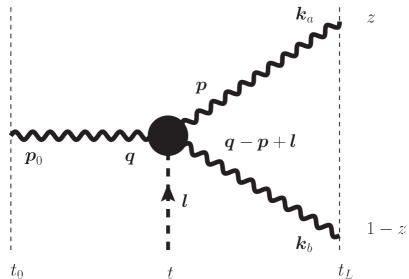
Figure 3: Graphical illustration of the equation (4). The thick wavy lines represent the probability ${\cal P}$ for transverse momentum broadening, the black dot is the splitting kernel ${\cal K}$.

The complete expression of the splitting kernel ${\cal K}({\bm{Q}},{\bm{l}},z,p_{0}^{+};t)$ is given in Appendix A, in terms of an integral representation obtained in the harmonic approximation (see Eq. (A)). Note that, in contrast to the fully integrated kernel in Eq. (16), the non integrated one is not positive definite anymore. (This is already obvious on the partially integrated one, Eq. (70), although we may argue that this particular kernel becomes negative only in a momentum region where it is dwarfed by the exponential.) Yet, even though strictly speaking one loses their probabilistic interpretation, the manipulations of the previous section can be formally repeated in order to obtain the evolution equation for the inclusive one-gluon distribution corresponding to a more general splitting kernel. This equation reads

$$\frac{\partial}{\partial t}D(x,{\bm{k}},t)=\int_{{\bm{l}}}\,{\cal C}({\bm{l}},t)D\left(x,{\bm{k}}-{\bm{l}},t\right)$$

$$+\alpha_{s}\int_{0}^{1}{\rm d}z\int_{{\bm{q}},{\bm{l}}}\bigg{[}2{\cal K}\left({\bm{Q}},{\bm{l}},z,\frac{x}{z}p^{+}_{0}\right)D\left(\frac{x}{z},{\bm{q}},t\right)-{\cal K}\left({\bm{q}},{\bm{l}},z,xp^{+}_{0}\right)D\left(x,{\bm{k}}-{\bm{l}},t\right)\bigg{]}\,,$$ (42)

where ${\bm{Q}}\equiv{\bm{k}}-z({\bm{q}}+{\bm{l}})$. In the following, we shall use the fact that ${\bm{Q}}$ and ${\bm{l}}$ are generically small compared to ${\bm{k}}$ in order to simplify this equation. The fact that ${\bm{l}}$ is small is obvious from its interpretation as the momentum broadening acquired during the branching process. That ${\bm{Q}}$ is also small may be inferred from the explicit expression (70) of the splitting kernel after integration over ${\bm{l}}$: this expression shows that the kernel which enters the ‘gain’ term in Eq. (4) is peaked around $|{\bm{Q}}|^{2}\sim k_{{}_{\rm br}}^{2}\equiv\sqrt{\omega_{0}\hat{q}_{0}}$, with $\omega_{0}=(1-z)xp_{0}^{+}$. The strategy that we shall follow then is the same as that we used in order to reduce Eq. (7) to the diffusion equation (9), which involves essentially an expansion around the large momentum ${\bm{k}}$ of the followed gluon.

4.1 The double logarithmic correction to $\hat{q}$

In order to perform this expansion in powers of the small momenta ${\bm{Q}}$ and ${\bm{l}}$, it is convenient to change variables in the r.h.s. of Eq. (4), in such a way that these momenta become the independent integration variables:

$$\frac{\partial}{\partial t_{L}}D(x,{\bm{k}},t_{L}) =\alpha_{s}\int_{0}^{1}{\rm d}z\int_{{\bm{Q}},{\bm{l}}}\,\bigg{[}\frac{2}{z^{2}}\,{\cal K}\left({\bm{Q}},{\bm{l}},z,\frac{x}{z}p^{+}_{0}\right)D\left(\frac{x}{z},({\bm{k}}-{\bm{Q}}-z{\bm{l}})/{z},t_{L}\right)$$

$$-{\cal K}\left({\bm{Q}},{\bm{l}},z,xp^{+}_{0}\right)D\left(x,{\bm{k}}-{\bm{l}},t_{L}\right)\bigg{]}-\int_{{\bm{l}}}\,{\cal C}({\bm{l}})D\left(x,{\bm{k}}-{\bm{l}},t_{L}\right)\,.$$ (43)

We can now expand the gluon distributions around ${\bm{k}}$. One gets, for the first term of Eq. (4.1),

$$D\left(\frac{x}{z},\frac{{\bm{k}}-\tilde{\bm{Q}}}{z}\right)=D\left(\frac{x}{z},\frac{{\bm{k}}}{z}\right)-\tilde{\bm{Q}}\cdot\frac{\partial}{\partial{\bm{k}}}D\left(\frac{x}{z},\frac{{\bm{k}}}{z}\right)+\frac{1}{2!}\,\tilde{Q}^{i}\tilde{Q}^{j}\frac{\partial}{\partial k_{i}}\frac{\partial}{\partial k_{j}}D\left(\frac{x}{z},\frac{{\bm{k}}}{z}\right)+\cdots$$ (44)

where we have set $\tilde{\bm{Q}}\equiv{\bm{Q}}+z{\bm{l}}$. One expands similarly $D\left(x,{\bm{k}}-{\bm{l}}\right)$. It is easy to see that the leading terms will reproduce Eq. (3.3). The linear terms will vanish upon angular integration. Remain the quadratic terms, whose contribution can be cast in the form of the diffusion term, thereby exhibiting a correction $\delta\hat{q}$ to the jet quenching parameter. For consistency, we shall also simplify the collision term by using the diffusion approximation.

The evolution equation obtained after this expansion to quadratic order reads

$$\frac{\partial}{\partial t_{L}}D(x,{\bm{k}},t_{L}) \,=\,\alpha_{s}\int_{0}^{1}{\rm d}z\,\bigg{[}\frac{2}{z^{2}}\,{\cal K}\left(z,\frac{x}{z}p^{+}_{0}\right)D\left(\frac{x}{z},\frac{{\bm{k}}}{z},t_{L}\right)-{\cal K}\left(z,xp^{+}_{0}\right)D\left(x,{\bm{k}},t_{L}\right)\bigg{]}$$

$$\quad+\frac{1}{4}\,\left(\frac{\partial}{\partial{\bm{k}}}\right)^{2}\big{[}\hat{q}({\bm{k}}^{2})\,D\left(x,{\bm{k}},t_{L}\right)\big{]}$$

$$\quad+\frac{1}{4}\,\left(\frac{\partial}{\partial{\bm{k}}}\right)^{2}\int_{x}^{1}{\rm d}z\,\frac{{\rm d}\delta\hat{q}(z,xp^{+}_{0},{\bm{k}}^{2})}{{\rm d}z}\,D\left(\frac{x}{z},\frac{{\bm{k}}}{z},t_{L}\right)\,,$$ (45)

where the first two lines are recognized as the leading–order transport equation, Eq. (3.3), and in the last term we have set

$$\frac{{\rm d}\delta\hat{q}(z,xp^{+}_{0},{\bm{k}}^{2})}{{\rm d}z} \equiv\frac{2\alpha_{s}}{z^{2}}\int_{{\bm{Q}},{\bm{l}}}\,({\bm{Q}}+z{\bm{l}})^{2}\,{\cal K}\left({\bm{Q}},{\bm{l}},z,\frac{x}{z}p^{+}_{0}\right)$$

$$-\alpha_{s}\delta(1-z)\int_{0}^{1}{\rm d}z^{\prime}\int_{{\bm{Q}},{\bm{l}}}\,{\bm{l}}^{2}\,{\cal K}({\bm{Q}},{\bm{l}},z^{\prime},xp^{+}_{0})\,.$$ (46)

The ${\bm{k}}^{2}$–dependence in Eq. (4.1) comes via the upper cutoff $\sim k$ in the integrals over ${\bm{Q}}$ and ${\bm{l}}$, which is kept implicit (see the discussion after Eq. (10), and Eq. (49) below).

The evaluation of the correction $\delta\hat{q}$ from Eq. (4.1) meets with logarithmic divergences. These arise from the region $z\lesssim 1$. To the leading-logarithmic accuracy, we can set $z=1$ everywhere, except in the dominant singularity. Thus the dominant contribution to $\delta\hat{q}$ can be then written as

$$\int_{x}^{1}{\rm d}z\,\frac{{\rm d}\delta\hat{q}(z,xp^{+}_{0},{\bm{k}}^{2})}{{\rm d}z}\,D\left(\frac{x}{z},\frac{{\bm{k}}}{z},t_{L}\right)\,\simeq\,\delta\hat{q}(x,{\bm{k}}^{2})\,D\left(x,{\bm{k}},t_{L}\right)\,,$$ (47)

with

$$\delta\hat{q}(x,{\bm{k}}^{2})\,\equiv\int_{x}^{1}{\rm d}z\,\frac{{\rm d}\delta\hat{q}(z,xp^{+}_{0},{\bm{k}}^{2})}{{\rm d}z}\,=\,2\alpha_{s}\int_{x}^{1}{\rm d}z\int_{{\bm{Q}},{\bm{l}}}\,\big{[}({\bm{Q}}+{\bm{l}})^{2}-{\bm{l}}^{2}\big{]}\,{\cal K}\left({\bm{Q}},{\bm{l}},z,xp^{+}_{0}\right),$$ (48)

where the lower limit $x$ in the integral over $z$, which was a priori present only in the ‘gain’ term, has also been inserted in the ‘loss’ term, while at the same time multiplying the latter by a factor of 2, to account for its original singularities at both $z=0$ and $z=1$ (which is legitimate since, to the accuracy of interest, the integral is controlled by values $z\simeq 1\gg x$). The particular combination of momenta, $\big{[}({\bm{Q}}+{\bm{l}})^{2}-{\bm{l}}^{2}\big{]}$, that emerges then in Eq. (48) can be given the following interpretation: when $z\simeq 1$, ${\bm{Q}}\equiv{\bm{k}}-z({\bm{q}}+{\bm{l}})$ is the same as (minus) the transverse momentum ${\bm{q}}+{\bm{l}}-{\bm{k}}$ of the unmeasured daughter gluon. Hence ${\bm{Q}}+{\bm{l}}\simeq{\bm{k}}-{\bm{q}}$ is the change in transverse momentum at the emission vertex, with two obvious components: the momentum ${\bm{l}}$ acquired via medium rescattering during the branching process and the momentum ${\bm{Q}}$ taken away by the unmeasured daughter gluon. The above applies to the ‘gain’ term. For the ‘loss’ term, there is no real emission, so the only source of momentum broadening is the momentum ${\bm{l}}$ transferred from the medium. The difference $({\bm{Q}}+{\bm{l}})^{2}-{\bm{l}}^{2}$ represents therefore the net change in the transverse momentum squared, and the average of this quantity over the (momentum dependent) splitting kernel yields the correction $\delta\hat{q}$.

The complete calculation of the integral (48) is presented in Appendix B, where it is shown that the result is dominated by the contribution of the single scattering to the splitting kernel. One gets

$$\delta\hat{q}({\bm{k}}^{2})=\frac{\alpha_{s}\,N_{c}}{2\pi}\,\hat{q}_{0}\,\ln^{2}\frac{{\bm{k}}^{2}}{\hat{q}\tau_{min}},$$ (49)

where $\tau_{min}$ is the inverse of the maximum energy that can be extracted from the medium in a single scattering (e.g. $\tau_{min}=1/T$ for a weakly coupled plasma with temperature $T$). This result agrees with that obtained in Ref. Liou:2013qya using a different approach.

The net result of incorporating this large radiative correction is a transport equation similar to that obtained at leading order, Eq. (3.3), but with an enhanced jet quenching coefficient, which includes the correction in Eq. (49) :

$$\frac{\partial}{\partial t_{L}}D(x,{\bm{k}},t_{L}) \,=\,\alpha_{s}\int_{0}^{1}{\rm d}z\,\bigg{[}\frac{2}{z^{2}}\,{\cal K}\left(z,\frac{x}{z}p^{+}_{0}\right)D\left(\frac{x}{z},\frac{{\bm{k}}}{z},t_{L}\right)-{\cal K}\left(z,xp^{+}_{0}\right)D\left(x,{\bm{k}},t_{L}\right)\bigg{]}$$

$$\quad+\frac{1}{4}\,\left(\frac{\partial}{\partial{\bm{k}}}\right)^{2}\big{[}\big{(}\hat{q}({\bm{k}}^{2})+\delta\hat{q}({\bm{k}}^{2})\big{)}\,D\left(x,{\bm{k}},t_{L}\right)\big{]}\,.$$ (50)

Note that the scale ${\bm{k}}^{2}$ which controls the size of the double logarithm is the transverse momentum accumulated by the gluon throughout the medium, that is ${\bm{k}}^{2}\sim Q_{s}^{2}=\hat{q}L$. Hence the argument of the logarithm is large, $\sim L/\tau_{min}$, which makes this radiative corrections particularly significant.

4.2 A logarithmic correction to $\hat{q}$

The correction that we have exhibited in the previous subsection appears to be the leading correction to the transport coefficient. There are also subleading (logarithmic, instead of double logarithmic) corrections. These have been estimated in Ref. Liou:2013qya , and could in principle be extracted as well from our calculation. In this section, we shall just focus on one particular logarithmic correction that is easy to obtain because it is the correction that naturally emerges when one uses the kernel integrated over ${\bm{l}}$ but not over ${\bm{Q}}$, namely the expression (70). The starting point is now the equation

$$\frac{\partial}{\partial t}D(x,{\bm{k}},t) =\int_{{\bm{l}}}\,{\cal C}({\bm{l}},t)D\left(x,{\bm{k}}-{\bm{l}},t\right)$$

$$+\alpha_{s}\int_{0}^{1}{\rm d}z\int_{{\bm{q}}}\bigg{[}2{\cal K}\left({\bm{Q}},z,\frac{x}{z}p^{+}_{0}\right)D\left(\frac{x}{z},{\bm{q}},t\right)-{\cal K}\left({\bm{q}},z,xp^{+}_{0}\right)D\left(x,{\bm{k}},t\right)\bigg{]}\,,$$ (51)

where ${\bm{Q}}\equiv{\bm{k}}-z{\bm{q}}$.

Expanding the distribution around the momentum ${\bm{k}}$ as in the previous subsection, one gets

$$\frac{\partial}{\partial t}D(x,{\bm{k}},t)-\frac{1}{4}\,\left(\frac{\partial}{\partial{\bm{k}}}\right)^{2}\big{[}\hat{q}({\bm{k}}^{2})D\left(x,{\bm{k}},t\right)\big{]}$$

$$=\alpha_{s}\int_{0}^{1}{\rm d}z\,\Bigg{[}\frac{2}{z^{2}}{\cal K}\left(z,\frac{x}{z}p^{+}_{0}\right)D\left(\frac{x}{z},\frac{{\bm{k}}}{z},t\right)-{\cal K}\left(z,xp^{+}_{0}\right)D\left(x,{\bm{k}},t\right)\bigg{]}$$

$$+\alpha_{s}\int_{0}^{1}{\rm d}z\int_{\bm{Q}}\frac{2}{z^{2}}{\cal K}\left({\bm{Q}},z,\frac{x}{z}p^{+}_{0}\right)\frac{1}{4}Q^{2}\frac{\partial^{2}}{\partial{\bm{k}}^{2}}D(x,{\bm{k}})$$ (52)

The second–order term in the expansion (which carries the divergence near $z=1$) yields a correction to $\hat{q}$, which we call $\delta\hat{q}^{\prime}$. We get (below, we use approximations valid for $z\simeq 1$)

$$\delta\hat{q}^{\prime} = 2\alpha_{s}\int_{x}^{1}{\rm d}z\int_{{\bm{Q}}}\,{\bm{Q}}^{2}\,{\cal K}\left({\bm{Q}},z,xp^{+}_{0}\right)$$ (53)

$$\propto \alpha_{s}\int_{x}^{1}{\rm d}z\,k_{{}_{\rm br}}^{4}(z,xp^{+}_{0})\,\frac{P(z)}{(1-z)xp_{0}^{+}}\,\sim\,\alpha_{s}\hat{q}\int_{x}^{1}\frac{{\rm d}z}{1-z}\,,$$

where to obtain the estimate in the second line we have used the fact that the splitting kernel is peaked at $k_{{}_{\rm br}}^{2}(z,xp^{+}_{0})=\sqrt{(1-z)xp_{0}^{+}\hat{q}}$, cf. Eq. (70). As anticipated, there is a logarithmic divergence at $z=1$, corresponding to $\omega_{0}\to 0$. This must be cut at the lowest energy scale at which the BDMPSZ mechanism is applicable, which is the Bethe–Heitler energy $\omega_{{}_{\rm BH}}\equiv\hat{q}_{0}\lambda_{{}_{\rm mfp}}$, i.e. the energy for which the branching time $\tau_{{}_{\rm br}}(\omega_{0})$ becomes of the order of the mean free path $\lambda_{{}_{\rm mfp}}$. In practice this means that the integral over $z$ in Eq. (53) must be restricted to $1-z\leq\omega_{{}_{\rm BH}}/\omega$, with $\omega=xp_{0}^{+}$ the energy of the measured gluon. Note that single scattering does not contribute to this logarithmic correction (as it can be checked using Eq. (A)), in contrast to the double logarithmic one discussed in the previous subsection. Let us also emphasize that Eq. (53) is only one among the several logarithmic corrections to $\hat{q}$ that have been analyzed in Ref. Liou:2013qya .

5 Conclusions

In this paper, we have extended our previous studies of the in-medium QCD cascade, based on the approximation that successive gluon branchings can be treated as independent from each other. This approximation is indeed justified for the typical partons within the cascade, whose formation times are much smaller than the medium size. We have constructed a generating functional for the various relevant probabilities and deduced from it the evolution equation for the inclusive one-gluon distribution function, that keeps track of the transverse momentum of the measured gluon. In this equation, however, the transverse momenta entering the splitting kernel are treated in an average way and the splittings are effectively collinear. This is justified since the transverse momentum broadening during the comparatively short (in our approximation, quasi–instantaneous) branching processes is much smaller than that accumulated via collisions in the medium all the way along the parton trajectories. By relaxing some of our approximations, in particular those which allow us to integrate the kernel over transverse momenta, we were able to identify large corrections to the jet quenching parameter, and in particular to recover the double logarithmic contribution that has been calculated recently in a general study of transverse momentum broadening.

Appendix A The splitting kernel

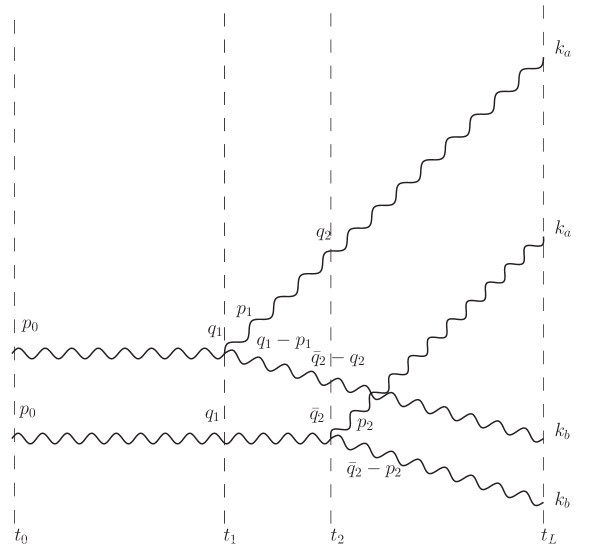
Figure 4: The momenta of the intermediate states in Eq. (A). The amplitude is drawn above the complex conjugate amplitude (see Ref. Blaizot:2012fh ), with the gluon splitting occurring at time $t_{1}$ in the amplitude, and at time $t_{2}$ in the complex conjugate amplitude. At any given time, the sum of momenta in the amplitude equals that of momenta in the complex conjugate amplitude.

It was shown in Ref. Blaizot:2012fh that the cross section for observing at time $t_{L}$ two gluons with momenta ${\vec{k}_{a}}$, $\vec{k}_{b}$, given that a single gluon was present with momentum $\vec{p}_{0}$ at time $t_{0}$, is given, in leading order perturbation theory, by

$$\frac{{\rm d}^{2}\sigma}{{\rm d}\Omega_{k_{a}}{\rm d}\Omega_{k_{b}}}=\int{\rm d}\Omega_{p_{0}}\,P_{2}(\vec{k}_{a},\vec{k}_{b};t_{L},t_{0})\,\frac{d\sigma_{hard}}{d\Omega_{p_{0}}},$$ (54)

where ${d\sigma_{hard}}/{d\Omega_{p_{0}}}$ is the hard cross section for the production of the initial gluon, and ${\rm d}\Omega_{k}\equiv(2\pi)^{-3}{\rm d}^{2}{\bm{k}}\,{\rm d}k^{+}/2k^{+}$ is the invariant phase–space element, and the vector notation $\vec{k}$ stands for $(p^{+},{\bm{p}})$, as in the main text of this paper. The probability $P_{2}(\vec{k}_{a},\vec{k}_{b};t_{L},t_{0})$ can be written as (cf. Eq. (14))

$$P_{2}(\vec{k}_{a},\vec{k}_{b};t_{L},t_{0})=2\pi\,2p_{0}^{+}\delta(k_{a}^{+}+k_{b}^{+}-p_{0}^{+})\,{\cal P}_{2}({\bm{k}}_{a},{\bm{k}}_{b},z;t_{L},t_{0}),$$ (55)

with $z=k_{a}^{+}/p_{0}^{+}$, and ${\cal P}_{2}({\bm{k}}_{a},{\bm{k}}_{b},z;t_{L},t_{0})$ given by

$${\cal P}_{2}({\bm{k}}_{a},{\bm{k}}_{b},z;t_{L},t_{0})=\frac{g^{2}P_{gg}(z)}{z(1-z)(p^{+}_{0})^{2}}\,2\Re e\,\int_{t_{0}}^{t_{L}}{\rm d}t_{2}\int_{t_{0}}^{t_{2}}{\rm d}t_{1}\,\int_{{\bm{p}}_{1}{\bm{q}}_{1}\bar{\bm{q}}_{2}{\bm{p}}_{2}{\bm{q}}_{2}}\,(\hat{\bm{P}}_{1}\cdot\hat{\bm{Q}}_{2})\,$$

$$\quad\times\,({\bm{k}}_{a}{\bm{k}}_{b};{\bm{k}}_{a}{\bm{k}}_{b}|\tilde{S}^{(4)}(t_{L},t_{2})|{\bm{q}}_{2},\bar{\bm{q}}_{2}-{\bm{q}}_{2};{\bm{p}}_{2},\bar{\bm{q}}_{2}-{\bm{p}}_{2})({\bm{q}}_{2},\bar{\bm{q}}_{2}-{\bm{q}}_{2};\bar{\bm{q}}_{2}|\tilde{S}^{(3)}(t_{2},t_{1})|{\bm{p}}_{1},{\bm{q}}_{1}-{\bm{p}}_{1};{\bm{q}}_{1})$$

$$\quad\times({\bm{q}}_{1};{\bm{q}}_{1}|\tilde{S}^{(2)}(t_{1},t_{0})|{\bm{p}}_{0};{\bm{p}}_{0}),$$ (56)

where $\hat{\bm{P}}_{1}\equiv{\bm{p}}_{1}-z{\bm{q}}_{1}$, $\hat{\bm{Q}}_{2}\equiv{\bm{p}}_{2}-z\bar{\bm{q}}_{2}$ denote the ‘natural’ momentum variables at the vertices in the amplitude and the complex conjugate amplitude, respectively. The explicit flow of momenta that label intermediate states is illustrated in Fig. 4. The dependence of ${\cal P}_{2}$ (and $P_{2}$) on the initial momentum $\vec{p}_{0}$ is left implicit to simplify the notation. The real part takes into account the time ordering $t_{1}>t_{2}$ not explicitly included in (A). The formula above has been obtained after performing the average over the field fluctuations using Eq. (1), and summing over polarizations. Azymuthal angles of the momenta at the vertices have also been averaged.

At this point no approximation has been made, except for the obvious restriction to leading order in perturbation theory (in the background field), that is, a single splitting occurs between $t_{0}$ and $t_{L}$. One may now introduce several approximations that are valid in the regime where the branching occurs on a time scale that is small compared to the length of the medium, i.e, in the regime $\tau_{{}_{\rm br}}\ll t_{L}-t_{0}$ (or equivalently for infinite medium length). We shall first consider the following two approximations:

1) Ignore the non factorizable piece of $\tilde{S}^{(4)}$, that is, set

$$({\bm{k}}_{a}{\bm{k}}_{b};{\bm{k}}_{a}{\bm{k}}_{b}|\tilde{S}^{(4)}_{\rm fac}(t_{L},t_{2})|{\bm{q}}_{2},\bar{\bm{q}}_{2}-{\bm{q}}_{2};{\bm{p}}_{2},\bar{\bm{q}}_{2}-{\bm{p}}_{2})$$

$$\qquad=(2\pi)^{2}\delta^{(2)}({\bm{p}}_{2}-{\bm{q}}_{2}){\cal P}({\bm{k}}_{a}-{\bm{q}}_{2},t_{L},t_{2}){\cal P}({\bm{k}}_{b}-\bar{\bm{q}}_{2}+{\bm{q}}_{2},t_{L},t_{2}).$$ (57)

It was shown in Blaizot:2012fh that the non factorizable piece of the 4-point function dies away over a time scale of order $\tau_{{}_{\rm br}}$, and it is down by a least one power of $\tau_{{}_{\rm br}}/L$ as compared to the factorized part.

2) Use as time integration variables $t_{1}$ and $t_{2}-t_{1}\equiv\tau$, i.e., set $t_{2}=t_{1}+\tau$, and neglect $\tau$ in the ${\cal P}$ factors that enter the 4-point function (57), that is e.g.

$${\cal P}({\bm{k}}_{a}-{\bm{q}}_{2},t_{L},t_{1}-\tau)\rightarrow{\cal P}({\bm{k}}_{a}-{\bm{q}}_{2},t_{L},t_{1}),$$ (58)

and similarly for the other ${\cal P}$. This allows us to integrate freely the 3-point function over $\tau$ from 0 to $\infty$ (as we shall soon recall, the 3-point function is strongly damped as soon as $\tau\gtrsim\tau_{{}_{\rm br}}$).
With these two approximations, Eq. (A) simplifies to

$${\cal P}_{2}({\bm{k}}_{a},{\bm{k}}_{b},z;t_{L},t_{0})=2g^{2}z(1-z)\,\int_{t_{0}}^{t_{L}}{\rm d}t_{1}\,\int_{{\bm{q}}_{1},\hat{\bm{Q}}_{2},{\bm{l}}}\;{\cal P}({\bm{k}}_{a}-{\bm{q}}_{2},t_{L},t_{1}){\cal P}({\bm{k}}_{b}-{\bm{q}}_{1}-{\bm{l}}+{\bm{q}}_{2},t_{L},t_{1})$$

$$\quad\quad\times\frac{P_{gg}(z)}{\omega_{0}^{2}}\,\Re e\left[\int_{\hat{\bm{P}}_{1}}\int_{0}^{\infty}{\rm d}\tau\,(\hat{\bm{P}}_{1}\cdot\hat{\bm{Q}}_{2})\,({\bm{q}}_{2},\bar{\bm{q}}_{2}-{\bm{q}}_{2};\bar{\bm{q}}_{2}|\tilde{S}^{(3)}(t_{2},t_{1})|{\bm{p}}_{1},{\bm{q}}_{1}-{\bm{p}}_{1};{\bm{q}}_{1})\right]$$

$$\quad\quad\times\,\,{\cal P}({\bm{q}}_{1}-{\bm{p}}_{0},t_{1}-t_{0}),$$ (59)

where we have set $\omega_{0}\equiv z(1-z)p_{0}^{+}$ and we have used as independent variables ${\bm{q}}_{1},\hat{\bm{P}}_{1}={\bm{p}}_{1}-z{\bm{q}}_{1},\hat{\bm{Q}}_{2}={\bm{p}}_{2}-z\bar{\bm{q}}_{2}={\bm{q}}_{2}-z\bar{\bm{q}}_{2},{\bm{l}}=\bar{\bm{q}}_{2}-{\bm{q}}_{1}$ in place of ${\bm{q}}_{1},{\bm{p}}_{1},\bar{\bm{q}}_{2},{\bm{q}}_{2}$. At this point we set (with a slight abuse of notation)

$$\tilde{S}^{(3)}(\hat{\bm{P}}_{1},\hat{\bm{Q}}_{2},{\bm{l}},z,\tau,t_{1})=({\bm{q}}_{2},\bar{\bm{q}}_{2}-{\bm{q}}_{2};\bar{\bm{q}}_{2}|\tilde{S}^{(3)}(t_{2},t_{1})|{\bm{p}}_{1},{\bm{q}}_{1}-{\bm{p}}_{1};{\bm{q}}_{1})$$ (60)

which makes explicit the relevant momentum variables on which the 3-point function depends, and we define the splitting kernel

$${\cal K}(\hat{\bm{Q}},{\bm{l}},z,t_{1})\,\equiv\,\frac{P_{gg}(z)}{\omega_{0}^{2}}\,{\rm Re}\int_{0}^{\infty}{\rm d}\tau\int_{\hat{\bm{P}}}(\hat{\bm{P}}\cdot\hat{\bm{Q}})\,\tilde{S}^{(3)}(\hat{\bm{P}},\hat{\bm{Q}},{\bm{l}},z,\tau,t_{1}).$$ (61)

With this new notation, Eq. (A) reads

$${\cal P}_{2}({\bm{k}}_{a},{\bm{k}}_{b},z;t_{L},t_{0})=2g^{2}z(1-z)\,\int_{t_{0}}^{t_{L}}{\rm d}t_{1}\,\int_{{\bm{q}}_{1},\hat{\bm{Q}}_{2},{\bm{l}}}\;{\cal P}({\bm{k}}_{a}-\hat{\bm{Q}}_{2}-z({\bm{q}}_{1}+{\bm{l}}),t_{L},t_{1})$$

$$\quad\quad\times{\cal P}({\bm{k}}_{b}+\hat{\bm{Q}}_{2}-(1-z)({\bm{q}}_{1}+{\bm{l}}),t_{L},t_{1})\;{\cal K}(\hat{\bm{Q}}_{2},{\bm{l}},z,t_{1})\,{\cal P}({\bm{q}}_{1}-{\bm{p}}_{0},t_{1},t_{0}).$$ (62)

At this point further approximations are legitimate. For instance, as we did in Blaizot:2012fh , we can neglect the momentum ${\bm{l}}$ in the ${\cal P}$ factors: indeed ${\bm{l}}$ represents the typical momentum acquired during the branching process, ${\bm{l}}^{2}\simeq\hat{q}\tau_{{}_{\rm br}}$, and it is small compared to $k_{a}$ or $k_{b}$ which are both of order $Q_{s}\sim\hat{q}(t_{L}-t_{0})$. If one neglects ${\bm{l}}$ in the ${\cal P}$ factors, then one can integrate the splitting kernel over ${\bm{l}}$ and get the simpler formula

$${\cal P}_{2}({\bm{k}}_{a},{\bm{k}}_{b},z;t_{L},t_{0})=2g^{2}z(1-z)\,\int_{t_{0}}^{t_{L}}{\rm d}t_{1}\,\int_{{\bm{q}}_{1},\hat{\bm{Q}}_{2}}\;{\cal P}({\bm{k}}_{a}-\hat{\bm{Q}}_{2}-z{\bm{q}}_{1},t_{L},t_{1})$$

$$\quad\quad\times{\cal P}({\bm{k}}_{b}+\hat{\bm{Q}}_{2}-(1-z){\bm{q}}_{1},t_{L},t_{1})\;{\cal K}(\hat{\bm{Q}}_{2},z)\,{\cal P}({\bm{q}}_{1}-{\bm{p}}_{0},t_{1},t_{0}).$$ (63)

with ${\cal K}(\hat{\bm{Q}},z,t)\equiv\int_{\bm{l}}{\cal K}(\hat{\bm{Q}},{\bm{l}},z,t)$. This is the approximation that was explicitly considered in Ref. Blaizot:2012fh .

We may also observe that the variable $\hat{\bm{Q}}$ that stands as argument of ${\cal K}$ is also small, of order $k_{{}_{\rm br}}\ll Q_{s}$, and can also be neglected in a leading order approximation. Doing so, one ends up with an even simpler formula

$${\cal P}_{2}({\bm{k}}_{a},{\bm{k}}_{b},z;t_{L},t_{0})=2g^{2}z(1-z)\,\int_{t_{0}}^{t_{L}}{\rm d}t_{1}\,{\cal K}(z,t_{1})\int_{{\bm{q}}_{1}}\;{\cal P}({\bm{k}}_{a}-z{\bm{q}}_{1},t_{L},t_{1})$$

$$\quad\quad\times{\cal P}({\bm{k}}_{b}-(1-z){\bm{q}}_{1},t_{L},t_{1})\;\,{\cal P}({\bm{q}}_{1}-{\bm{p}}_{0},t_{1},t_{0}).$$ (64)

with ${\cal K}(z,t)\equiv\int_{\hat{\bm{Q}}}{\cal K}(\hat{\bm{Q}},z,t)=\int_{{\bm{Q}}{\bm{l}}}{\cal K}(\hat{\bm{Q}},{\bm{l}},z,t)$ is the fully integrated splitting kernel. This is the kernel used to construct the generating functional of the in-medium cascade in Sect. 3.

As was shown in Blaizot:2012fh , the 3-point function can be written as the following path integral

$$\tilde{S}^{(3)}({\bm{P}},{\bm{Q}},{\bm{l}},z,p_{0}^{+};t_{2},t_{1})=\int{\rm d}{\bm{u}}_{1}{\rm d}{\bm{u}}_{2}{\rm d}{\bm{v}}\;{\rm e}^{i{\bm{u}}_{1}\cdot{\bm{P}}-i{\bm{u}}_{2}\cdot{\bm{Q}}-i{\bm{v}}\cdot{\bm{l}}}$$

$$\times\int_{{\bm{u}}_{1}}^{{\bm{u}}_{2}}{\cal D}{\bm{u}}\exp\left\{\frac{i\omega_{0}}{2}\int_{t_{1}}^{t_{2}}{\rm d}t~{}\dot{{\bm{u}}}^{2}-\frac{N_{c}}{4}\int_{t_{1}}^{t_{2}}{\rm d}t\,n(t)\left[\sigma({\bm{u}})+\sigma({\bm{v}}-z{\bm{u}})+\!\sigma({\bm{v}}+(1-z){\bm{u}})\right]\right\}.$$

This can be explicitly evaluated within the ‘harmonic approximation’, which assumes $\sigma({\bm{r}})\propto\hat{q}{\bm{r}}^{2}$ (cf. Eq. (11)). By expanding all the $\sigma$’s to quadratic order, and performing the resulting gaussian path integrals, one gets Blaizot:2012fh

$$\tilde{S}^{(3)}({\bm{P}},{\bm{Q}},{\bm{l}},z,p_{0}^{+};t_{2},t_{1})=\frac{16\pi f(z)}{3\hat{q}\Delta t}\exp\left\{-\frac{4f(z)\big{[}{\bm{l}}+(1-2z)({\bm{P}}-{\bm{Q}})/2f(z)\big{]}^{2}}{3\hat{q}\Delta t}\right\}$$

$$\quad\times\ \frac{2\pi i}{\Omega\omega_{0}\sinh(\Omega\Delta t)}\exp\left\{-i\frac{({\bm{P}}+{\bm{Q}})^{2}}{4\omega_{0}\Omega\coth(\Omega\Delta t/2)}-i\frac{({\bm{P}}-{\bm{Q}})^{2}}{4\omega_{0}\Omega\tanh(\Omega\Delta t/2)}\right\}\,.$$ (66)

where $\Delta t\equiv t_{2}-t_{1}$, $f(z)\equiv 1-z(1-z)$, and

$$\Omega\equiv\,\frac{1+i}{2\tau_{{}_{\rm br}}(z,p^{+}_{0})},$$ (67)

with $\tau_{{}_{\rm br}}(z,p^{+}_{0})\equiv\sqrt{{\omega_{0}}/{\hat{q}_{0}}}$ and $\hat{q}_{0}\equiv\hat{q}f(z)$.

By inserting the result (A) for $\tilde{S}^{(3)}$ into Eq. (61), one finds the following integral representation for the splitting kernel (in the harmonic approximation):

$${\cal K}({\bm{Q}},{\bm{l}},z,p_{0}^{+};t)\,=\,{16\pi}\,\frac{f(z)P_{gg}(z)}{\omega_{0}^{2}}\,\Re e\int_{0}^{\infty}\frac{{\rm d}\Delta t}{3\hat{q}\Delta t}\,$$

$$\times\int_{{\bm{P}}}\,({\bm{Q}}\cdot{\bm{P}})\,{\exp}\left\{-\frac{4f(z)\,\big{[}{\bm{l}}+(1-2z)({\bm{P}}-{\bm{Q}})/2f(z)\big{]}^{2}}{3\hat{q}\Delta t}\right\}$$

$$\times\frac{2\pi i}{\Omega\omega_{0}\sinh(\Omega\Delta t)}\exp{\left\{-i\frac{({\bm{P}}+{\bm{Q}})^{2}}{4\omega_{0}\Omega\coth(\Omega\Delta t/2)}-i\frac{({\bm{P}}-{\bm{Q}})^{2}}{4\omega_{0}\Omega\tanh(\Omega\Delta t/2)}\right\}}.$$ (68)

This kernel obeys the symmetry property:

$${\cal K}({\bm{Q}},{\bm{l}},z,p_{0}^{+};t)\,=\,{\cal K}(-{\bm{Q}},{\bm{l}},1-z,p_{0}^{+};t)\,,$$ (69)

which expresses the symmetry of the splitting under the exchange of the two daughter gluons.

By performing the integration over ${\bm{l}}$ one recovers the splitting kernel obtained in Blaizot:2012fh :

$${\cal K}({\bm{Q}},z,p_{0}^{+};t)\equiv\int_{\bm{l}}{\cal K}({\bm{Q}},{\bm{l}},z,p_{0}^{+};t)=\frac{2}{p_{0}^{+}}\frac{P_{gg}(z)}{z(1-z)}\,\sin\left[\frac{{\bm{Q}}^{2}}{2k_{{}_{\rm br}}^{2}}\right]\exp\left[-\frac{{\bm{Q}}^{2}}{2k_{{}_{\rm br}}^{2}}\right],$$ (70)

In this expression, $k_{{}_{\rm br}}^{2}=\hat{q}_{0}\tau_{{}_{\rm br}}(z,p^{+}_{0})=\sqrt{\omega_{0}\hat{q}_{0}}$ is the typical transverse momentum squared transferred via medium rescattering during the splitting. Note that the branching time, and hence the splitting kernel, depend upon both $p_{0}^{+}$ (the energy of the parent gluon) and upon the splitting fraction $z$. The expression (70) illustrates an important property of the branching that is induced by soft multiple collisions: it is strongly peaked at $|{\bm{Q}}|\sim k_{{}_{\rm br}}(z,p^{+}_{0})$. For smaller momenta $|{\bm{Q}}|\ll k_{{}_{\rm br}}$, gluon splitting is suppressed by $Q^{2}/k_{{}_{\rm br}}^{2}$, which reflects the interferences of the LPM effect. At larger momenta $|{\bm{Q}}|\gtrsim k_{{}_{\rm br}}$, it is rapidly damped, as it is unlikely to acquire more transverse momentum than $k_{{}_{\rm br}}$ via multiple scattering.

The kernel in Eq. (70) contains information about the geometry of the medium–induced splitting: the polar angles made by the two offspring gluons with respect to their parent parton are $\theta_{z}\simeq|{\bm{Q}}|/zp_{0}^{+}$ and respectively $\theta_{1-z}\simeq|{\bm{Q}}|/(1-z)p_{0}^{+}$. Since $|{\bm{Q}}|\sim k_{{}_{\rm br}}\ll Q_{s}=\sqrt{\hat{q}L}$, it is clear that these angles are negligible compared to the angular spreading acquired via collisions in between successive branchings. By integrating the kernel (70) over ${\bm{Q}}$, this information about the emission angles is averaged out, and one obtains the fully integrated kernel ${\cal K}(z,p_{0}^{+};t)$ given explicitly in Eq. (16).

Finally, we shall write the expression of the splitting kernel in the limit where a single scattering occurs during the branching process. We limit ourselves to the case where $z\lesssim 1$, the case of relevance for discussing the double logarithmic correction to $\hat{q}$. The three-point function in the one-scattering approximation, obtained by expanding (A) to leading order in $\sigma$, takes the form

$$\tilde{S}^{(3)}({\bm{P}},{\bm{Q}},{\bm{l}})\approx-\frac{N_{c}}{4}\int_{t_{1}}^{t_{2}}{{\rm d}}t\,n(t)\,{\cal G}_{0}({\bm{Q}},t_{2}-t)\,{\cal G}_{0}({\bm{P}},t-t_{1})$$

$$\times\left[(2\pi)^{2}\delta({\bm{l}})\,\sigma({\bm{Q}}-{\bm{P}})+(2\pi)^{2}\delta({\bm{Q}}-{\bm{P}}+{\bm{l}})\,\sigma({\bm{l}})+(2\pi)^{2}\delta({\bm{Q}}-{\bm{P}})\,\sigma({\bm{l}})\right],$$

where ${\cal G}_{0}({\bm{Q}},t_{2}-t_{1})$ is the free propagator

$${\cal G}_{0}({\bm{Q}},t_{2}-t_{1})={\rm e}^{-i\frac{{\bm{Q}}^{2}}{2\omega_{0}}(t_{2}-t_{1})}.$$ (72)

When needed (see below) a small negative imaginary part may be added to ${\bm{Q}}^{2}$ to account for the retarded condition. If we assume that $n$ is independent of time, we can perform the time integration, and obtain ($\tau\equiv t_{2}-t_{1}$)

$$\tilde{S}^{(3)}({\bm{P}},{\bm{Q}},{\bm{l}})\approx-\frac{N_{c}n\omega_{0}}{2i}\,\frac{{\rm e}^{-i\frac{{\bm{P}}^{2}}{2\omega_{0}}\tau}-{\rm e}^{-i\frac{{\bm{Q}}^{2}}{2\omega_{0}}\tau}}{Q^{2}-P^{2}}$$

$$\times\left[(2\pi)^{2}\delta({\bm{l}})\,\sigma({\bm{Q}}-{\bm{P}})+(2\pi)^{2}\delta({\bm{Q}}-{\bm{P}}+{\bm{l}})\,\sigma({\bm{l}})+(2\pi)^{2}\delta({\bm{Q}}-{\bm{P}})\,\sigma({\bm{l}})\right].$$

At this point, the kernel reads

$${\cal K}({\bm{Q}},{\bm{l}},z)\,\equiv\,\frac{C_{A}^{2}n}{1-z}\,{\rm Re}\int_{{\bm{P}}}\frac{{\bm{P}}\cdot{\bm{Q}}}{Q^{2}P^{2}}$$

$$\times\left[(2\pi)^{2}\delta({\bm{l}})\,\sigma({\bm{Q}}-{\bm{P}})+(2\pi)^{2}\delta({\bm{Q}}-{\bm{P}}+{\bm{l}})\,\sigma({\bm{l}})+(2\pi)^{2}\delta({\bm{Q}}-{\bm{P}})\,\sigma({\bm{l}})\right].$$

where we have used the time integral (recall that $P^{2}\to P^{2}-i\epsilon$)

$$\int_{0}^{\infty}{\rm d}\tau\,\frac{{\rm e}^{-i\frac{{\bm{P}}^{2}}{2\omega_{0}}\tau}-{\rm e}^{-i\frac{{\bm{Q}}^{2}}{2\omega_{0}}\tau}}{Q^{2}-P^{2}}=-\frac{2i\omega_{0}}{Q^{2}P^{2}}.$$ (75)

This expression will be used in the next Appendix. Note that the last two terms in the r.h.s of Eq. (A) vanish upon integration over ${\bm{l}}$, because of the identities (6). These terms play an essential role in the evaluation of $\delta\hat{q}$, as shown in the next Appendix.

Appendix B Estimating the double logarithmic correction to $\hat{q}$

Our starting point is the integral representation for the kernel given, in the harmonic approximation, by Eq. (A), where we keep only the singular part at $z\to 1$ from the Altarelli–Parisi splitting function $P_{gg}(z)$ (see Eq. (17)), and we set $z=1$ in the rest of the expression. After inserting Eq. (A) into the r.h.s. of Eq. (48), we are facing four integrations: an integration over the duration $\tau$ of the branching process and three Gaussian integrations over the momentum variables ${\bm{l}}$, ${\bm{Q}}$ and ${\bm{P}}$. Performing first the integral over ${\bm{l}}$, one obtains (with $\tau\equiv\Delta t$)

$$\delta\hat{q}({\bm{k}}^{2})\simeq 2\alpha_{s}\,\Re e\int_{x}^{1}\frac{dz}{1-z}\frac{C_{A}}{\omega^{2}_{0}}\int_{0}^{\infty}{\rm d}\tau\int_{{\bm{Q}},{\bm{P}}}\,({\bm{Q}}\cdot{\bm{P}})^{2}\,$$

$$\times\frac{2\pi i}{\omega_{0}\Omega\sinh(\Omega\tau)}\exp{\left\{-i\frac{({\bm{P}}+{\bm{Q}})^{2}}{4\omega_{0}\Omega\coth(\Omega\tau/2)}-i\frac{({\bm{P}}-{\bm{Q}})^{2}}{4\omega_{0}\Omega\tanh(\Omega\tau/2)}\right\}},$$ (76)

where $\omega_{0}\equiv(1-z)zq^{+}\simeq(1-z)xp^{+}_{0}$ and $\omega_{0}\Omega^{2}=i\hat{q}_{0}/2$ (cf. Eq. (67)). Note that for $z$ close to one, the quantity $\omega_{0}$ is essentially the energy $(1-z)q^{+}$ of the unresolved gluon and $\hat{q}_{0}\simeq\hat{q}$. It is now straightforward to perform the remaining momentum integrations, yielding

$$\delta\hat{q}({\bm{k}}^{2})=2\,\Re e\int_{x}^{1}\frac{dz}{1-z}\frac{\alpha_{s}\,C_{A}}{\omega^{2}_{0}}\int_{0}^{\infty}{\rm d}\tau\,\frac{i(\omega_{0}\Omega)^{3}}{\pi}\frac{1}{\sinh(\Omega\tau)}\left[1+\frac{4}{\sinh^{2}(\Omega\tau)}\right].$$ (77)

Anticipating on the fact that the dominant (divergent) contribution will come from the small $\tau$ region, we carefully expand the integrand for $|\Omega|\tau\ll 1$ and get

$$\frac{\Omega^{3}}{\sinh\Omega\tau}\,\left(1+\frac{4}{\sinh^{2}\Omega\tau}\right)\approx\frac{4}{\tau^{3}}-\frac{\Omega^{2}}{\tau}.$$ (78)

The $\Omega$–independent piece is real, so it does not contribute to the real part of the integral in Eq. (77) (because of the explicit factor $i$ in Eq. (77)). The second term in the r.h.s. Eq. (78) is purely imaginary and is linear in $\hat{q}_{0}$, suggesting that it describes the contribution of a single scattering (see below). When inserted into Eq. (77), this term generates an integral which is logarithmically divergent as $\tau\to 0$. One then gets, after changing the integration variable from $z$ to $\omega_{0}=(1-z)xp^{+}_{0}$,

$$\delta\hat{q}({\bm{k}}^{2}) \approx \frac{\alpha_{s}\,N_{c}}{\pi}\,\hat{q}\,\int\frac{{\rm d}\omega_{0}}{\omega_{0}}\int\frac{{\rm d}\tau}{\tau}\,.$$ (79)

We can verify that the dominant contribution to ${\cal K}$ is coming from a single scattering with the medium by using the expression obtained in Appendix A, Eq. (A), in order to perform the calculation. We get (with $\omega_{0}=(1-z)p^{+}$)

$$\omega_{0}\frac{\rm d\delta\hat{q}}{{\rm d}\omega_{0}} = 2\alpha_{s}\int_{{\bm{Q}},{\bm{l}}}\,{\bm{q}}\cdot({\bm{Q}}+2{\bm{l}})\,{\cal K}({\bm{Q}},{\bm{l}},z)$$ (80)

$$= 4\alpha_{s}N_{c}^{2}n\,{\rm Re}\int_{{\bm{Q}},{\bm{P}}}\frac{({\bm{Q}}\cdot{\bm{P}})^{2}}{{\bm{Q}}^{2}{\bm{P}}^{2}}\sigma({\bm{Q}}-{\bm{P}})$$

where, in order to perform the ${\bm{l}}$ integration we have used the identities (6). By using Eq. (5), we get

$$\int_{{\bm{Q}},{\bm{Q}}}\frac{({\bm{Q}}\cdot{\bm{P}})^{2}}{{\bm{Q}}^{2}{\bm{P}}^{2}}\sigma({\bm{Q}}-{\bm{P}}) = 2g^{2}\int_{{\bm{q}},{\bm{l}}}\,\gamma({\bm{l}})\frac{{\bm{Q}}^{2}{\bm{l}}^{2}-({\bm{l}}\cdot{\bm{Q}})^{2}}{{\bm{Q}}^{2}({\bm{Q}}-{\bm{l}})^{2}}$$ (81)

$$\approx g^{2}\int_{{\bm{Q}}}\,\frac{1}{{\bm{Q}}^{2}}\,\int_{\bm{l}}{\bm{l}}^{2}\gamma({\bm{l}}),$$

where, in the last line, we have made approximations valid in the region $l\ll Q$. We therefore get from (80)

$$\omega_{0}\frac{\rm d\delta\hat{q}}{{\rm d}\omega_{0}} = 2\alpha_{s}N_{c}^{2}n\,\int_{{\bm{Q}}}\,\frac{1}{{\bm{Q}}^{2}}\,\int_{\bm{l}}{\bm{l}}^{2}V({\bm{l}})$$ (82)

$$= \frac{\alpha N_{c}}{\pi}\,\hat{q}\,\int\frac{{\rm d}{\bm{Q}}^{2}}{{\bm{Q}}^{2}},$$

which is recognized as Eq. (79) after recalling that the formation time and the virtuality of the soft emitted gluon are related by $\tau\simeq\omega_{0}/Q^{2}$.

Returning to Eq. (79), we shall now discuss the boundaries of the double integral there. Consider the time integral first. At larger times $|\Omega|\tau\gtrsim 1$, this integral is cutoff by the exponential decay of $[\sinh\Omega\tau]^{-1}$ ; this is the effect of multiple scattering during the emission process, which limits the branching times to values $\tau\lesssim\tau_{{}_{\rm br}}(\omega_{0})=\sqrt{\omega_{0}/\hat{q}}$. On the other hand the time $\tau$ cannot be smaller that the inverse of the maximum energy that can be taken away from the medium through a single scattering Liou:2013qya . We call this limiting time $\tau_{min}$. This lower bound may not always be reached however. If $\omega_{0}$ is not too small, then $\tau$ will be limited by the formation time of the unobserved gluon, $\tau\simeq\omega_{0}/Q_{\perp}^{2}$. But in reality such values cannot exceed the transverse momentum $k_{\perp}$ of the measured gluon, which in turn implies a lower limit $\sim\omega_{0}/k_{\perp}^{2}$ in the integral over $\tau$. Thus the lower bound on $\tau$ is ${\rm max}\,\big{(}\tau_{min},\,\omega_{0}/k_{\perp}^{2}\big{)}$.

Turning now to $\omega_{0}$, we note that the lower limit at $z=x$ in the original integral over $z$ implies an upper limit $\omega_{0}^{\rm max}=(1-x)xp^{+}_{0}\simeq xp^{+}_{0}=\omega$ (the energy of the measured gluon) in the integral over $\omega_{0}$. For the ensuing integral to have a non–trivial support when $\tau=\tau_{min}$, one also needs $\tau_{{}_{\rm br}}(\omega_{0})\equiv\sqrt{\omega_{0}/\hat{q}}\,\gtrsim\tau_{min}$, that is, $\omega_{0}\gtrsim\hat{q}\tau_{min}^{2}$.

In view of the above, we need to split the integral over $\omega_{0}$ into two regions:

$$\hat{q}_{1}({\bm{k}}^{2}) \approx \frac{\alpha_{s}\,N_{c}}{\pi}\,\hat{q}\,\left\{\int_{\hat{q}\tau_{min}^{2}}^{\tau_{min}{\bm{k}}^{2}}\frac{{\rm d}\omega_{0}}{\omega_{0}}\int_{\tau_{min}}^{\sqrt{\omega_{0}/\hat{q}}}\frac{{\rm d}\tau}{\tau}\,+\int_{\tau_{min}{\bm{k}}^{2}}^{\omega}\frac{{\rm d}\omega_{0}}{\omega_{0}}\int_{\omega_{0}/{\bm{k}}^{2}}^{\sqrt{\omega_{0}/\hat{q}}}\frac{{\rm d}\tau}{\tau}\right\}.$$ (83)

$$\approx \frac{\alpha_{s}\,N_{c}}{2\pi}\,\hat{q}\,\left\{\ln^{2}\frac{{\bm{k}}^{2}}{\hat{q}\tau_{min}}-\frac{1}{2}\ln^{2}\frac{{\bm{k}}^{4}}{\hat{q}\omega}\right\}.$$ (84)

Dropping the last term (negligible if $\omega\gg\tau_{min}{\bm{k}}^{2}$), one finds the result (49).

Appendix C Equivalence between forward and backward evolutions

As mentioned earlier, one may write two types of evolution equations, depending on whether one differentiates the generating functional with respect to the initial of the final times. These two evolutions are referred to as backward and forward Kolmogorov evolutions (see Ref. (Cvitanovic:1980ru ) for a general discussion). In section 3, we have discussed the forward case. We discuss here the backward case that is often preferred for Monte-Carlo implementations. The two formulations are in principle equivalent, although the forms of the resulting equations may look rather different. At the end of this Appendix, we shall prove the equivalence in the case of the inclusive one gluon distribution.

In order to derive the backward evolution equation for the generating functional, which we denote now ${\cal Z}[p^{+},{\bm{p}};t_{L},t_{0}|u]$, we first note the analog of Eq. (3.2) for the time derivative of ${\cal P}_{2}$, with now the derivative acting on $t_{0}$:

$$-\partial_{t_{0}}{\cal P}_{2}({\bm{k}}_{a},{\bm{k}}_{b},z;t_{L},t_{0})$$

$$\qquad=2g^{2}z(1-z){\cal K}(z,p_{0}^{+};t_{0}){\cal P}({\bm{k}}_{a}-z{\bm{p}}_{0};t_{L},t_{0}){\cal P}({\bm{k}}_{b}-(1-z){\bm{p}}_{0};t_{L},t_{0}).$$ (85)

This provides the essential ingredient for the construction of the evolution equation, which reads:

$$-\frac{\partial}{\partial t_{0}}{\cal Z}[\vec{p};t_{L},t_{0}|u] = \alpha_{s}\int_{0}^{1}{\rm d}z\,{\cal K}(z,p^{+};t_{0})\Big{\{}{\cal Z}[z\vec{p};t_{L},t_{0}|u]\,{\cal Z}[(1-z)\vec{p};t_{L},t_{0}|u]-{\cal Z}[\vec{p};t_{L},t_{0}|u]\Big{\}}$$ (86)

$$+ \int_{{\bm{l}}}{\cal C}({\bm{l}},t_{0}){\cal Z}[p^{+},{\bm{p}}-{\bm{l}};t_{L},t_{0}|u]\,.$$

The term quadratic in ${\cal Z}$ within the braces in the r.h.s. describes the splitting of the initial parton into two partons, whereas the term linear in ${\cal Z}$ is necessary to ensure probability conservation. As usual, the collision term which involves ${\cal C}$ accounts for transverse momentum broadening.

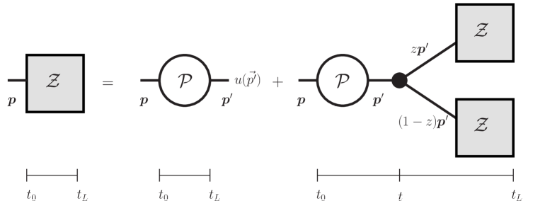
Figure 5: Diagrammatic representation of the master equation (C)

This differential equation can easily be transformed into an integral equation, which reads

$${\cal Z}[\vec{p};t_{L},t_{0}|u]=\int_{{\bm{p}}^{\prime}}\,\Delta(p^{+};t_{L}-t_{0}){\cal P}({\bm{p}}^{\prime}-{\bm{p}};t_{L},t_{0})\,u(p^{+},{\bm{p}}^{\prime})$$

$$+\alpha_{s}\int_{t_{0}}^{t_{L}}{\rm d}t\,\int_{{\bm{p}}^{\prime}}\Delta(p^{+};t-t_{0}){\cal P}({\bm{p}}^{\prime}-{\bm{p}};t_{L},t_{0})$$

$$\times\int_{0}^{1}{\rm d}z\,{\cal K}(z,p^{+},t)\,{\cal Z}\big{[}zp^{+},z{\bm{p}}^{\prime};t_{L},t|u\big{]}\ {\cal Z}\big{[}(1-z)p^{+},(1-z){\bm{p}}^{\prime};t_{L},t|u\big{]}\,,$$

where $\Delta(p^{+};t_{L}-t_{0})$ is the Sudakov factor defined in Eq. (31). This equation, which is graphically illustrated in Fig. 5, recursively generates the ensemble of the cascade by ‘inserting one additional splitting at the beginning of the cascade’.

As an illustration of the equivalence between the two different versions for the evolution equations, we show explicitly the connection between them for the specific case of the one-gluon energy distribution.

The evolution equation for the one-gluon energy distribution, as derived from the generating functional, reads

$$-\frac{\partial}{\partial\tau_{0}}D(x,\tau-\tau_{0})=\int^{1}_{0}dz\,\hat{\cal K}(z)\,D\left({x\over z},{\tau-\tau_{0}\over\sqrt{z}}\right)-\frac{1}{2}\int^{1}_{0}dz\,\hat{\cal K}(z)\,D\left(x,\tau-\tau_{0}\right)\,.$$ (88)

It is understood, here and in the following equation that $D(x>1)=0$, so that the lower bound on the first $z$-integration is actually $z=x$. To write down this equation we have assumed that the energy of the initial parton is $p_{0}^{+}$. It is convenient, for the foregoing derivation, to consider an arbitrary initial $p^{+}$, so that we shift $p_{0}^{+}$ to $x^{\prime}p_{0}^{+}$. Under such a shift $\tau\rightarrow\tau/\sqrt{x^{\prime}}$ (recall Eq. (38)). We can then rewrite Eq. (88) as

$$-\frac{\partial}{\partial\tau_{0}}D\left({x\over x^{\prime}},{\tau-\tau_{0}\over\sqrt{x^{\prime}}}\right)=\frac{1}{\sqrt{x^{\prime}}}\int^{1}_{0}dz\,\hat{\cal K}(z)\,D\left({x\over zx^{\prime}},{\tau-\tau_{0}\over\sqrt{zx^{\prime}}}\right)-\frac{1}{2\sqrt{x^{\prime}}}\int^{1}_{0}dz\,\hat{\cal K}(z)\,D\left({x\over x^{\prime}},{\tau-\tau_{0}\over\sqrt{x^{\prime}}}\right).$$

Now let us introduce the following identity (which results from the Chapman-Kolmogorov law of composition of probabilities)

$$D(x,\tau-\tau_{0})=\int_{x}^{1}\frac{dx^{\prime}}{x^{\prime}}\,D\left({x\over x^{\prime}},{\tau-\tau^{\prime}\over\sqrt{x^{\prime}}}\right)D(x^{\prime},\tau^{\prime}-\tau_{0}).$$ (90)

This equality holds for any $\tau^{\prime}$. In particular, it is obviously true for $\tau^{\prime}=\tau_{0}$ where $D(x^{\prime},0)=\delta(x^{\prime}-1)$, and for $\tau^{\prime}=\tau$ where $D(x/x^{\prime},0)=x\delta(x-x^{\prime})$. More generally, taking the derivative of Eq. (90) with respect to $\tau^{\prime}$ one gets

$$-\int_{x}^{1}\frac{{\rm d}x^{\prime}}{x^{\prime}}\,\frac{\partial}{\partial\tau^{\prime}}D\left({x\over x^{\prime}},{\tau-\tau^{\prime}\over\sqrt{x^{\prime}}}\right)D(x^{\prime},\tau^{\prime}-\tau_{0})=\int_{x}^{1}\frac{{\rm d}x^{\prime}}{x^{\prime}}\,D\left({x\over x^{\prime}},{\tau-\tau^{\prime}\over\sqrt{x^{\prime}}}\right)\frac{\partial}{\partial\tau^{\prime}}D(x^{\prime},\tau^{\prime}-\tau_{0}).$$

By combining this equation with Eq. (C) (in which we replace $\tau_{0}$ by $\tau^{\prime}$) we get

$$\int_{x}^{1}\frac{{\rm d}x^{\prime}}{x^{\prime}}D\left({x\over x^{\prime}},{\tau-\tau^{\prime}\over\sqrt{x^{\prime}}}\right)\frac{\partial}{\partial\tau^{\prime}}D(x^{\prime},\tau^{\prime}-\tau_{0}) = \int_{x}^{1}\frac{{\rm d}x^{\prime}}{x^{\prime}}\frac{1}{\sqrt{x^{\prime}}}\int^{1}_{0}dz\hat{\cal K}(z)\,D\left({x\over zx^{\prime}},{\tau-\tau^{\prime}\over\sqrt{zx^{\prime}}}\right)D(x^{\prime},\tau^{\prime}-\tau_{0})$$

$$- \int_{x}^{1}\frac{{\rm d}x^{\prime}}{x^{\prime}}\frac{1}{2\sqrt{x^{\prime}}}\int^{1}_{0}dz\hat{\cal K}(z)\,D\left({x\over x^{\prime}},{\tau-\tau^{\prime}\over\sqrt{x^{\prime}}}\right)D(x^{\prime},\tau^{\prime}-\tau_{0})\,.$$

At this point we set $\tau^{\prime}=\tau$, which allows us to perform the $x^{\prime}$ integrations (thanks to the properties recalled after Eq. (90)). We end up with

$$\frac{\partial}{\partial\tau}D(x,\tau-\tau_{0})=\int^{1}_{x}dz\,\hat{\cal K}(z)\,\sqrt{\frac{z}{x}}\,D\left(\frac{x}{z},\tau-\tau_{0}\right)-\frac{1}{2\sqrt{x}}\int^{1}_{0}dz\,\hat{\cal K}(z)\,D(x,\tau-\tau_{0}).$$ (93)

Since $\hat{\cal K}(z)$ is symmetric under the transformation $z\to 1-z$, we have

$$\int_{0}^{1}dz\,z\hat{\cal K}(z)=\int_{0}^{1}dz\,(1-z)\hat{\cal K}(z)=\frac{1}{2}\int_{0}^{1}dz\,\hat{\cal K}(z)\,,$$ (94)

which allows us to write Eq. (93) as

$$\frac{\partial}{\partial\tau}D(x,\tau)=\int^{1}_{x}dz\,\hat{\cal K}(z)\,\sqrt{\frac{z}{x}}\,D\left(\frac{x}{z},\tau\right)-\int^{1}_{0}dz\,\frac{z}{\sqrt{x}}\hat{\cal K}(z)\,D(x,\tau),$$

which is the evolution equation (40).

References

• (1) Atlas Collaboration Collaboration, G. Aad et. al., Observation of a Centrality-Dependent Dijet Asymmetry in Lead-Lead Collisions at $\sqrt{s_{NN}}=2.77$ TeV with the ATLAS Detector at the LHC, Phys.Rev.Lett. 105 (2010) 252303, [arXiv:1011.6182].
• (2) CMS Collaboration Collaboration, S. Chatrchyan et. al., Observation and studies of jet quenching in PbPb collisions at nucleon-nucleon center-of-mass energy = 2.76 TeV, Phys.Rev. C84 (2011) 024906, [arXiv:1102.1957].
• (3) CMS Collaboration Collaboration, S. Chatrchyan et. al., Jet momentum dependence of jet quenching in PbPb collisions at $\sqrt{s_{NN}}=2.76$ TeV, Phys.Lett. B712 (2012) 176–197, [arXiv:1202.5022].
• (4) ATLAS Collaboration Collaboration, G. Aad et. al., Measurement of the jet radius and transverse momentum dependence of inclusive jet suppression in lead-lead collisions at $\sqrt{s_{NN}}$= 2.76 TeV with the ATLAS detector, Phys.Lett. B719 (2013) 220–241, [arXiv:1208.1967].
• (5) CMS Collaboration Collaboration, S. Chatrchyan et. al., Modification of jet shapes in PbPb collisions at $\sqrt{s_{NN}}$ = 2.76 TeV, arXiv:1310.0878.
• (6) R. Baier, Y. L. Dokshitzer, A. H. Mueller, S. Peigne, and D. Schiff, Radiative energy loss of high-energy quarks and gluons in a finite volume quark - gluon plasma, Nucl.Phys. B483 (1997) 291–320.
• (7) R. Baier, Y. L. Dokshitzer, A. H. Mueller, S. Peigne, and D. Schiff, Radiative energy loss and p(T) broadening of high-energy partons in nuclei, Nucl.Phys. B484 (1997) 265–282.
• (8) R. Baier, Y. L. Dokshitzer, A. H. Mueller, and D. Schiff, Medium induced radiative energy loss: Equivalence between the BDMPS and Zakharov formalisms, Nucl.Phys. B531 (1998) 403–425, [hep-ph/9804212].
• (9) B. Zakharov, Fully quantum treatment of the Landau-Pomeranchuk-Migdal effect in QED and QCD, JETP Lett. 63 (1996) 952–957.
• (10) B. Zakharov, Radiative energy loss of high-energy quarks in finite size nuclear matter and quark - gluon plasma, JETP Lett. 65 (1997) 615–620.
• (11) U. A. Wiedemann, Gluon radiation off hard quarks in a nuclear environment: Opacity expansion, Nucl.Phys. B588 (2000) 303–344, [hep-ph/0005129].
• (12) M. Gyulassy, P. Levai, and I. Vitev, Reaction operator approach to nonAbelian energy loss, Nucl.Phys. B594 (2001) 371–419, [nucl-th/0006010].
• (13) P. B. Arnold, G. D. Moore, and L. G. Yaffe, Photon and gluon emission in relativistic plasmas, JHEP 0206 (2002) 030, [hep-ph/0204343].
• (14) Y. Mehtar-Tani, C. A. Salgado, and K. Tywoniuk, Anti-angular ordering of gluon radiation in QCD media, Phys.Rev.Lett. 106 (2011) 122002, [arXiv:1009.2965].
• (15) Y. Mehtar-Tani, C. Salgado, and K. Tywoniuk, Jets in QCD Media: From Color Coherence to Decoherence, Phys.Lett. B707 (2012) 156–159, [arXiv:1102.4317].
• (16) J. Casalderrey-Solana and E. Iancu, Interference effects in medium-induced gluon radiation, JHEP 1108 (2011) 015, [arXiv:1105.1760].
• (17) Y. Mehtar-Tani, C. A. Salgado, and K. Tywoniuk, The radiation pattern of a QCD antenna in a dilute medium, JHEP 1204 (2012) 064, [arXiv:1112.5031].
• (18) Y. Mehtar-Tani and K. Tywoniuk, Jet coherence in QCD media: the antenna radiation spectrum, JHEP 1301 (2013) 031, [arXiv:1105.1346].
• (19) J. Casalderrey-Solana, Y. Mehtar-Tani, C. A. Salgado, and K. Tywoniuk, New picture of jet quenching dictated by color coherence, Phys.Lett. B725 (2013) 357–360, [arXiv:1210.7765].
• (20) J.-P. Blaizot, F. Dominguez, E. Iancu, and Y. Mehtar-Tani, Medium-induced gluon branching, JHEP 1301 (2013) 143, [arXiv:1209.4585].
• (21) J.-P. Blaizot, E. Iancu, and Y. Mehtar-Tani, Medium-induced QCD cascade: democratic branching and wave turbulence, Phys.Rev.Lett. 111 (2013) 052001, [arXiv:1301.6102].
• (22) T. Liou, A. Mueller, and B. Wu, Radiative $p_{\bot}$-broadening of high-energy quarks and gluons in QCD matter, Nucl.Phys. A916 (2013) 102–125, [arXiv:1304.7677].
• (23) G. Altarelli and G. Parisi, Asymptotic Freedom in Parton Language, Nucl.Phys. B126 (1977) 298.
• (24) P. Cvitanovic, P. Hoyer, and K. Zalewski, Parton evolution as a branching process, Nucl.Phys. B176 (1980) 429.
• (25) R. Baier, A. H. Mueller, D. Schiff, and D. Son, ’Bottom up’ thermalization in heavy ion collisions, Phys.Lett. B502 (2001) 51–58, [hep-ph/0009237].
• (26) S. Jeon and G. D. Moore, Energy loss of leading partons in a thermal QCD medium, Phys.Rev. C71 (2005) 034901, [hep-ph/0309332].
• (27) B. Schenke, C. Gale, and S. Jeon, MARTINI: An Event generator for relativistic heavy-ion collisions, Phys.Rev. C80 (2009) 054913, [arXiv:0909.2037].