Elastodynamics and resonances in elliptical geometry

Abstract

The resonant modes of two-dimensional elastic elliptical objects are studied from a modal formalism by emphasizing the role of the symmetries of the objects. More precisely, as the symmetry is broken in the transition from the circular disc to the elliptical one, splitting up of resonances and level crossings are observed. From the mathematical point of view, this observation can be explained by the broken invariance of the continuous symmetry group ${\mathcal{O}(2)}$ associated to the circular disc. The elliptical disc is however invariant under the finite group ${\mathcal{C}}_{2v}$ and the resonances are classified and associated with a given irreducible representation of this group. The main difficulty stands in the application of the group theory in elastodynamics where the vectorial formalism is used to express the physical quantities (elastic displacement and stress) involved in the boundary conditions. However, this method significantly simplifies the numerical treatment of the problem which is uncoupled over the four irreducible representations of ${\mathcal{C}}_{2v}$. This provides a full classification of the resonances. They are tagged and tracked as the eccentricity of the elliptical disc increases. Then, the splitting up of resonances, which occurs in the transition from the circular disc to the elliptic one, is emphasized. The computation of vibrational normal modes displacement also highlights mode splittings. A physical interpretation of resonances in terms of geometrical paths is provided.

1 Introduction

Resonant modes of elastic objects have been extensively studied in the last decades, more particularly for simple shapes [1]. In 1882, Lamb was the first to solve exactly the problem of the free vibrations of an elastic isotropic and homogeneous sphere [2]. Visscher et al. [3] introduced a method based on Hamilton’s principle approach to compute resonant modes of elastic objects for various geometries. More recently, Saviot and Murray [4] focused on the classification of the spheroidal vibrational modes of an elastic sphere. In the context of classical ray dynamics, Tanner and Søndergaard studied the eigenfrequencies of an elastic circular disc [5] and their connection to the periodic rays in the circular domain. Little attention has been given to the elliptical geometry in elastodynamics comparatively to acoustic scattering [6]. However, many techniques ($S$ matrix [7], modal formalism [8]) employed in this latter context can be transposed to the interior problem.

In this paper, the elastodynamic resonances of elliptical objects are studied from a modal formalism. In the scalar case, by using the appropriate elliptic coordinates, the Helmholtz equation separates into two equations involving Mathieu functions [9, 10]. Unfortunately, in elastodynamics, the Helmholtz equation does not separate in elliptic coordinates due to the existence of longitudinal and transverse waves [7, 11]. This brings us to use circular cylinder coordinates $(\rho,\theta,z)$. Then we shall assume that the problem is independent of the $z$-coordinate and thus reduces to a two-dimensional one, referred as plain strain, the elliptical disc, described by the polar coordinates $(\rho,\theta)$.

Several authors have paid attention to the role of the symmetries in various contexts [12, 13, 14, 10]. The present work deals with the resonant modes of the elastic elliptical disc, focusing on the splitting up of resonances which occurs in the transition from the circular disc to the elliptical one. In terms of group theory, this corresponds to the symmetry breaking $\mathcal{O}(2)$ $\rightarrow$ $\mathcal{C}_{2v}$. This splitting up has been numerically observed for the first time by Moser and Überall [15]. More recently, Chinnery and Humphrey discussed about mode splittings and level crossings in the study of the acoustic resonances of a submerged fluid-filled cylindrical shell [16]. However, none of these authors provides an explanation or analytical description to this phenomenon. In the scalar case, Ancey et al [10, 17] have highlighted and explained the splitting up of resonances in the elliptical geometry using a method involving group theory [18]. This technique has also been used to study multiple scattering [13, 14]. The main advantages of this method stand in (i) the uncoupling of the equations, (ii) the classification of resonances, (iii) the highlighting of the splitting up of resonances and its interpretation in terms of symmetry breaking.

The paper is organized as follows. In section 2, the geometry of the problem is presented and algebraic considerations are recalled. Then, from the boundary condition, four systems of equations are obtained, each one associated with a given irreducible representation of the symmetry group $\mathcal{C}_{2v}$. The problem is uncoupled and these systems can then be solved numerically by truncation and used to obtain the resonances. In section 3, numerical results are presented for the resonances. They are tracked as the eccentricity of the elliptical disc increases and splitting up of resonances is emphasized. The computation of vibrational normal modes displacement also highlights the mode splittings. Finally, a physical interpretation in terms of periodic orbits is given and the phenomenon of mode conversion is observed.

2 Mathematical Formalism

2.1 Position of the problem

Let us consider an elastic elliptical disc. The elastic medium is characterized by the longitudinal and transverse velocities $c_{L}$ and $c_{T}$ and we introduce the wave numbers $k_{L}=\omega/c_{L}$ and $k_{T}=\omega/c_{T}$, where $\omega$ is the angular frequency. The time dependence $e^{-i\omega t}$ is assumed throughout the paper. As explained in section 1, we shall use the polar coordinates ($\rho$, $\theta$). The geometry as well as the notations used are displayed in figure 1. The elliptical boundary is a closed curved described by the radius $r(\theta)$ with a continuously turning outward normal $\mathbf{n}(\theta)$ defined by

$$\mathbf{n}(\theta)=n_{\rho}\mathbf{e}_{\rho}+n_{\theta}\mathbf{e}_{\theta}$$ (1)

with

$$n_{\rho}=\frac{1-e^{2}\cos^{2}\theta}{\sqrt{1+e^{2}(e^{2}-2)\cos^{2}\theta}},\;\;\;\;\;n_{\theta}=\frac{e^{2}}{2}\frac{\sin 2\theta}{\sqrt{1+e^{2}(e^{2}-2)\cos^{2}\theta}}$$ (2)

and

$$r(\theta)=\frac{b}{\sqrt{1-e^{2}\cos^{2}\theta}}$$ (3)

where $e^{2}=1-\frac{b^{2}}{a^{2}}$ defines the eccentricity $e$ (figure 1).

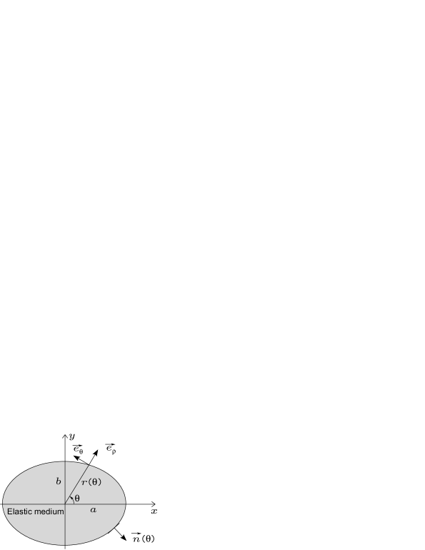
Figure 1: Geometry of the problem.

The elastic displacement $\mathbf{u}$ is expressed using the Helmholtz decomposition:

$$\mathbf{u}=-\mathbf{\nabla}\phi+\mathbf{\nabla}\wedge\mathbf{\psi}$$ (4)

where $\phi$ and $\mathbf{\psi}=\psi\mathbf{e}_{z}$ are the scalar and vectorial potentials respectively associated with the longitudinal and transverse fields. The scalar potentials $\phi$ and $\psi$ satisfy the Helmholtz equations $\nabla^{2}\phi+k_{L}^{2}\phi=0$ and $\nabla^{2}\psi+k_{T}^{2}\psi=0$. Since the longitudinal and transverse fields in the elastic elliptical disc have no singularity in the neighbourhood of the origin, they can be expanded in terms of Bessel functions as

$$\phi=\sum_{n=-\infty}^{+\infty}A_{n}^{L}J_{n}(k_{L}\rho)e^{in\theta},\;\;\;\;\;\psi=\sum_{n=-\infty}^{+\infty}A_{n}^{T}J_{n}(k_{T}\rho)e^{in\theta}$$ (5)

where $A_{n}^{j}$ are unknown coefficients with $j\in\{L,T\}$. The physical quantity to consider in what follows is the elastic displacement expressed by

$$\mathbf{u}=u_{\rho}\mathbf{e}_{\rho}+u_{\theta}\mathbf{e}_{\theta}=\left(-\frac{\partial\phi}{\partial\rho}+\frac{1}{\rho}\frac{\partial\psi}{\partial\theta}\right)\mathbf{e}_{\rho}+\left(-\frac{1}{\rho}\frac{\partial\phi}{\partial\theta}-\frac{\partial\psi}{\partial\rho}\right)\mathbf{e}_{\theta}.$$ (6)

2.2 Symmetry considerations and group theory

We extend to a vectorial formalism a method already used in the context of a scalar theory [13, 14, 10]. The elliptical disc is invariant under four symmetry transformations (figure 2): (i) $E$, the identity transformation $\left(\theta\rightarrow\theta\right)$, (ii) $C_{2}$, the rotation through $\pi$ about the $Oz$ axis $\left(\theta\rightarrow\pi+\theta\right)$, (iii) $\sigma_{x}$, the mirror reflection in the plane $Oxz$ $\left(\theta\rightarrow-\theta\right)$, (iv) $\sigma_{y}$, the mirror reflection in the plane $Oyz$ $\left(\theta\rightarrow\pi-\theta\right)$.

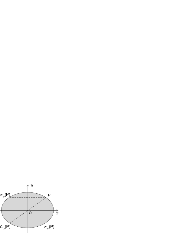
Figure 2: Symmetry transformations.

These four transformations form a finite group, called $\mathcal{C}_{2v}$, which is the symmetry group of the elliptical disc [18]. The action of these transformations on the basis vectors $\mathbf{e}_{\rho}$ and $\mathbf{e}_{\theta}$ is given by

$$E(\mathbf{e}_{\rho}) = \mathbf{e}_{\rho};\quad C_{2}(\mathbf{e}_{\rho})=\mathbf{e}_{\rho};\quad\sigma_{x}(\mathbf{e}_{\rho})=\mathbf{e}_{\rho};\quad\;\;\sigma_{y}(\mathbf{e}_{\rho})=\mathbf{e}_{\rho}$$ (7a)

$$E(\mathbf{e}_{\theta}) = \mathbf{e}_{\theta};\quad C_{2}(\mathbf{e}_{\theta})=\mathbf{e}_{\theta};\quad\sigma_{x}(\mathbf{e}_{\theta})=-\mathbf{e}_{\theta};\quad\sigma_{y}(\mathbf{e}_{\theta})=-\mathbf{e}_{\theta}$$ (7b)

Four one-dimensional irreducible representations labelled $A_{1}$, $A_{2}$, $B_{1}$, $B_{2}$ are associated with this symmetry group $\mathcal{C}_{2v}$. In a given representation ($A_{1}$, $A_{2}$, $B_{1}$ or $B_{2}$) the group elements $E$, $C_{2}$, $\sigma_{x}$ and $\sigma_{y}$ are represented by $1\times 1$ matrices given in the corresponding row of the character table (table 1)

Table 1: Character table of $\mathcal{C}_{2v}$.

$\mathcal{C}_{2v}:$	$E$	$C_{2}$	$\sigma_{x}$	$\sigma_{y}$
$A_{1}$	1	1	1	1
$A_{2}$	1	1	1	1
$B_{1}$	1	1	1	1
$B_{2}$	1	1	1	1

. From the character table 1, we can obviously deduce, by applying the four symmetry transformations to the basis vectors, that $\mathbf{e}_{\rho}$ belongs to the representation $A_{1}$ and $\mathbf{e}_{\theta}$ belongs to the representation $A_{2}$.

Let us consider a vectorial function $\mathbf{f}(\rho,\theta)$ expressed in the polar coordinates system as

$$\mathbf{f}(\rho,\theta)=f_{\rho}\mathbf{e}_{\rho}+f_{\theta}\mathbf{e}_{\theta}.$$ (7h)

The character table permits one to split the scalar components $f_{\rho},f_{\theta}$ as a sum of functions belonging to the four irreducible representations of $\mathcal{C}_{2v}$. Indeed, one can write

$$f_{i}(\rho,\theta)=f_{i}^{A_{1}}(\rho,\theta)+f_{i}^{A_{2}}(\rho,\theta)+f_{i}^{B_{1}}(\rho,\theta)+f_{i}^{B_{2}}(\rho,\theta)\;_{;}\;i\in\{\rho,\theta\}$$ (7i)

with $f_{i}^{A_{1}}(\rho,\theta)$, $f_{i}^{A_{2}}(\rho,\theta)$, $f_{i}^{B_{1}}(\rho,\theta)$, $f_{i}^{B_{2}}(\rho,\theta)$ satisfying

$$Ef_{i}^{A_{1}} = f_{i}^{A_{1}};\quad C_{2}f_{i}^{A_{1}}=f_{i}^{A_{1}};\quad\;\;\sigma_{x}f_{i}^{A_{1}}=f_{i}^{A_{1}};\quad\;\;\sigma_{y}f_{i}^{A_{1}}=f_{i}^{A_{1}}$$ (7ja)

$$Ef_{i}^{A_{2}} = f_{i}^{A_{2}};\quad C_{2}f_{i}^{A_{2}}=f_{i}^{A_{2}};\quad\;\;\sigma_{x}f_{i}^{A_{2}}=-f_{i}^{A_{2}};\quad\sigma_{y}f_{i}^{A_{2}}=-f_{i}^{A_{2}}$$ (7jb)

$$Ef_{i}^{B_{1}} = f_{i}^{B_{1}};\quad C_{2}f_{i}^{B_{1}}=-f_{i}^{B_{1}};\quad\sigma_{x}f_{i}^{B_{1}}=f_{i}^{B_{1}};\quad\;\;\sigma_{y}f_{i}^{B_{1}}=-f_{i}^{B_{1}}$$ (7jc)

$$Ef_{i}^{B_{2}} = f_{i}^{B_{2}};\quad C_{2}f_{i}^{B_{2}}=-f_{i}^{B_{2}};\quad\sigma_{x}f_{i}^{B_{2}}=-f_{i}^{B_{2}};\quad\sigma_{y}f_{i}^{B_{2}}=f_{i}^{B_{2}}.$$ (7jd)

Hence, the vectorial function can be expressed as

$$\mathbf{f}(\rho,\theta)=\left(f_{\rho}^{A_{1}}+f_{\rho}^{A_{2}}+f_{\rho}^{B_{1}}+f_{\rho}^{B_{2}}\right)\mathbf{e}_{\rho}+\left(f_{\theta}^{A_{1}}+f_{\theta}^{A_{2}}+f_{\theta}^{B_{1}}+f_{\theta}^{B_{2}}\right)\mathbf{e}_{\theta},$$ (7jk)

where the symmetry decomposition over $A_{1},$ $A_{2},$ $B_{1},$ $B_{2}$ is only carried out for the scalar components.

Since group theory will be applied to the displacement vector $\mathbf{u,}$ we need to generalize the decomposition over the four irreducible representations in a purely vector context. Expanding equation (7jk), by taking into account that $\mathbf{e}_{\rho}\in A_{1}$ and $\mathbf{e}_{\theta}\in A_{2},$ and according to the multiplication table 2, one can write $\mathbf{f}(\rho,\theta)$ as a sum of vector functions, each belonging to a given irreducible representation of $\mathcal{C}_{2v},$ in the form

$$\mathbf{f}(\rho,\theta)=\mathbf{f}^{A_{1}}(\rho,\theta)+\mathbf{f}^{A_{2}}(\rho,\theta)+\mathbf{f}^{B_{1}}(\rho,\theta)+\mathbf{f}^{B_{2}}(\rho,\theta),$$ (7jl)

with

$$\mathbf{f}^{A_{1}} = f_{\rho}^{A_{1}}\mathbf{e}_{\rho}+f_{\theta}^{A_{2}}\mathbf{e}_{\theta}$$ (7jma)

$$\mathbf{f}^{A_{2}} = f_{\rho}^{A_{2}}\mathbf{e}_{\rho}+f_{\theta}^{A_{1}}\mathbf{e}_{\theta}$$ (7jmb)

$$\mathbf{f}^{B_{1}} = f_{\rho}^{B_{1}}\mathbf{e}_{\rho}+f_{\theta}^{B_{2}}\mathbf{e}_{\theta}$$ (7jmc)

$$\mathbf{f}^{B_{2}} = f_{\rho}^{B_{2}}\mathbf{e}_{\rho}+f_{\theta}^{B_{1}}\mathbf{e}_{\theta}.$$ (7jmd)

It should be noted that the scalar components of a vectorial function in a given irreducible representation do not necessarily belong to the same representation (see (7jma-7jmd)).

Table 2: Multiplication table for a function belonging to a given irreducible representation.

$\times$	$A_{1}$	$A_{2}$	$B_{1}$	$B_{2}$
$A_{1}$	$A_{1}$	$A_{2}$	$B_{1}$	$B_{2}$
$A_{2}$	$A_{2}$	$A_{1}$	$B_{2}$	$B_{1}$
$B_{1}$	$B_{1}$	$B_{2}$	$A_{1}$	$A_{2}$
$B_{2}$	$B_{2}$	$B_{1}$	$A_{2}$	$A_{1}$

The use of group theory allows us to restrict the study to the so-called fundamental domain which reduces to a quarter of the elliptical disc $\theta\in\left[0,\pi/2\right]$ (see figure 3). This constitutes a great improvement from both theoretical and numerical point of view. Of course, the physical quantities of interest can be determined for the full domain from simple symmetry considerations (table 1).

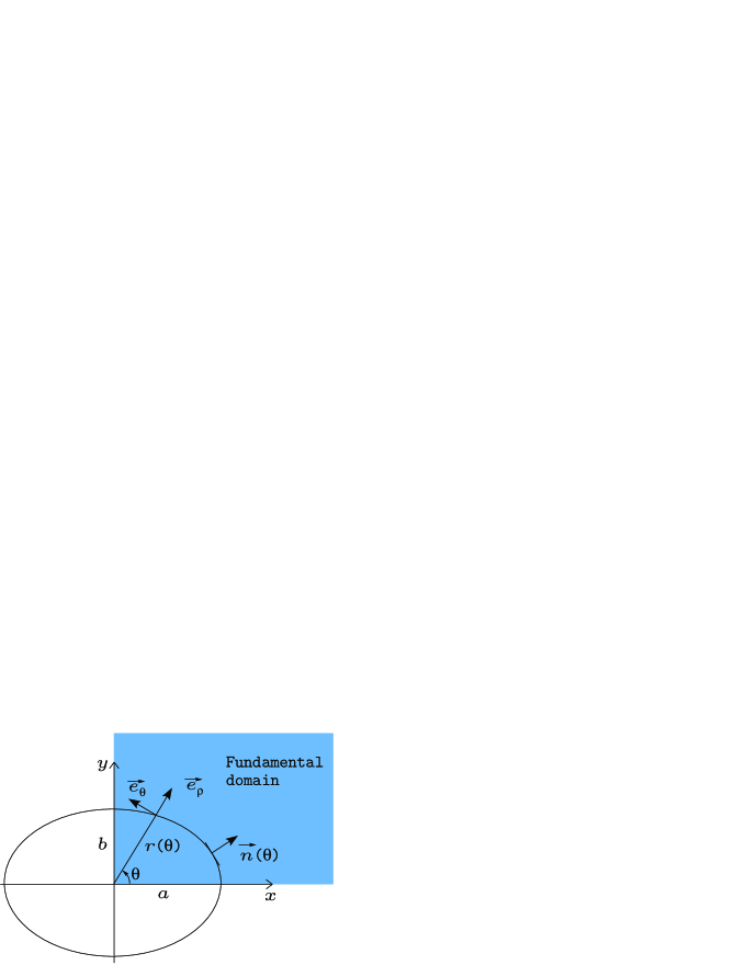
Figure 3: Fundamental domain.

2.3 Solving the eigenvalue problem

The eigenfrequencies are calculated by applying the traction-free boundary condition $\mathbf{t}=\overline{\overline{\mathbf{\sigma}}}\cdot\mathbf{n}(\theta)=\mathbf{0}$ on the ellipse $\rho=r(\theta)$, i.e.

$$t_{\rho}\mathbf{e}_{\rho}+t_{\theta}\mathbf{e}_{\theta}=\mathbf{0}$$ (7jmn)

with, according to equation (1),

$$t_{\rho} = \sigma_{\rho\rho}n_{\rho}+\sigma_{\rho\theta}n_{\theta},$$ (7jmoa)

$$t_{\theta} = \sigma_{\rho\theta}n_{\rho}+\sigma_{\theta\theta}n_{\theta}.$$ (7jmob)

The components of $\overline{\overline{\mathbf{\sigma}}}$ in circular cylindrical coordinates are obtained from the strain tensor [19], Hooke’s law, and the Helmholtz equation for the scalar potential $\phi$

$$\sigma_{\rho\rho} = \lambda k_{L}^{2}\phi-2\mu\biggl{(}\frac{\partial^{2}\phi}{\partial\rho^{2}}+\frac{1}{\rho^{2}}\frac{\partial\psi}{\partial\theta}-\frac{1}{\rho}\frac{\partial^{2}\psi}{\partial\rho\partial\theta}\biggr{)},$$ (7jmopa)

$$\sigma_{\rho\theta} = \sigma_{\theta\rho}=\mu\biggl{(}-\frac{2}{\rho}\frac{\partial^{2}\phi}{\partial\theta\partial\rho}+\frac{1}{\rho^{2}}\frac{\partial^{2}\psi}{\partial\theta^{2}}+\frac{1}{\rho}\frac{\partial\psi}{\partial\rho}-\frac{\partial^{2}\psi}{\partial\rho^{2}}+\frac{2}{\rho^{2}}\frac{\partial\phi}{\partial\theta}\biggr{)},$$ (7jmopb)

$$\sigma_{\theta\theta} = \lambda k_{L}^{2}\phi+2\mu\biggl{(}-\frac{1}{\rho^{2}}\frac{\partial^{2}\phi}{\partial\theta^{2}}-\frac{1}{\rho}\frac{\partial^{2}\psi}{\partial\theta\partial\rho}-\frac{1}{\rho}\frac{\partial\phi}{\partial\rho}+\frac{1}{\rho^{2}}\frac{\partial\psi}{\partial\theta}\biggr{)}.$$ (7jmopc)

The boundary condition (7jmn) can now be expressed separately in each irreducible representation. We note that $\mathbf{n}(\theta)$ defined by (1) belongs to $A_{1}$ for obvious symmetry considerations, thus its components $n_{\rho}$ and $n_{\theta}$ respectively belong to $A_{1}$ and $A_{2}$ under the property (7jma). In what follows, we use the latter property, the multiplication table (table 2) and we note that the derivative by respect to $\theta$ acts as a multiplication by some function belonging to the representation $A_{2}$.

For clarity, we also define

$$\sum_{n\;\mathit{even}}f_{n}:=\sum_{r=0}^{+\infty}f_{2r},\;\;\;\mathit{and}\;\sum_{n\;\mathit{odd}}f_{n}:=\sum_{r=0}^{+\infty}f_{2r+1}.$$ (7jmopq)

2.3.1 Representation $A_{1}$

We express the boundary condition $\mathbf{t}=\mathbf{0}$ in the irreducible representation $A_{1}$, using (7jma) with $\phi^{A_{1}}$ and $\psi^{A_{2}}$ satisfying (7ja) and (7jb) given by

$$\phi^{A_{1}}(\rho,\theta)=\sum_{n\;\mathit{even}}\gamma_{n}A_{n}^{L}J_{n}(k_{L}\rho)\cos n\theta,\;\;\;\;\;\psi^{A_{2}}(\rho,\theta)=\sum_{n\;\mathit{even}}\gamma_{n}A_{n}^{T}J_{n}(k_{T}\rho)\sin n\theta,$$ (7jmopr)

where $\gamma_{n}$ is the Neumann factor defined by $\gamma_{0}=1$ and $\gamma_{n}=2$ for $n>0.$ We obtain

$$\sum_{n\;\mathit{even}}\gamma_{n}\left[A_{n}^{L}\left(c_{n}^{L}n_{\rho}\cos n\theta+d_{n}^{L}n_{\theta}\sin n\theta\right)+A_{n}^{T}\left(c_{n}^{T}n_{\rho}\cos n\theta+d_{n}^{T}n_{\theta}\sin n\theta\right)\right] = 0$$ (7jmopsa)

$$\sum_{n\;\mathit{even}}\gamma_{n}\left[A_{n}^{L}\left(d_{n}^{L}n_{\rho}\sin n\theta-f_{n}^{L}n_{\theta}\cos n\theta\right)+A_{n}^{T}\left(d_{n}^{T}n_{\rho}\sin n\theta-f_{n}^{T}n_{\theta}\cos n\theta\right)\right] = 0$$ (7jmopsb)

where the structural functions $c_{n}^{j},$ $d_{n}^{j},$ $f_{n}^{j},$ $j\in\{L,T\}$ are given in A. To overcome the angular dependence, the functions $F_{n}(\theta)$ in parenthesis appearing in (7jmopsa) and (7jmopsb) are expanded in Fourier series by setting

$$F_{n}(\theta)=\sum_{p=-\infty}^{+\infty}f_{n,p}e^{ip\theta},\;\;\;\mathit{with}\;f_{n,p}=\frac{1}{2\pi}\int_{-\pi}^{\pi}F_{n}(\theta)e^{-ip\theta}d\theta.$$ (7jmopst)

In (7jmopst), the restriction to the fundamental domain and the parity of $F_{n}(\theta)$ permits one to reduce the domain of integration from $\left[-\pi,\pi\right]$ to $\left[0,\pi/2\right]$ and the sum over $p$ from $\left[-\infty,+\infty\right]$ to $\left[0,+\infty\right]$ with $p$ even. Then (7jmopsa) and (7jmopsb) lead to the final equations

$$\sum_{n\;\mathit{even}}\sum_{p\;\mathit{even}}\gamma_{n}\gamma_{p}\left(A_{n}^{L}\,\beta_{n,p}^{L}+A_{n}^{T}\,\beta_{n,p}^{T}\right)\cos p\theta=0$$ (7jmopsua)

$$\sum_{n\;\mathit{even}}\sum_{p\;\mathit{even}}\gamma_{n}\left(A_{n}^{L}\,\xi_{n,p}^{L}+A_{n}^{T}\,\xi_{n,p}^{T}\right)\sin p\theta=0$$ (7jmopsub)

where the Fourier coefficients $\beta_{n,p}^{j},\xi_{n,p}^{j}$, $j\in\{L,T\}$ are given in B.

Proceeding by a similar way, we obtain mutatis mutandis the final equations for the representations $A_{2},$ $B_{1}$ and $B_{2}.$

2.3.2 Representation $A_{2}$

Using (7jmb), $\phi^{A_{2}}$ and $\psi^{A_{1}}$ satisfying (7ja) and (7jb) given by

$$\phi^{A_{2}}(\rho,\theta)=\sum_{n\;\mathit{even}}\gamma_{n}A_{n}^{L}J_{n}(k_{L}\rho)\sin n\theta,\;\;\;\;\;\psi^{A_{1}}(\rho,\theta)=\sum_{n\;\mathit{even}}\gamma_{n}A_{n}^{T}J_{n}(k_{T}\rho)\cos n\theta,$$ (7jmopsuv)

the boundary condition reads

$$\sum_{n\;\mathit{even}}\gamma_{n}\left[A_{n}^{L}\left(c_{n}^{L}n_{\rho}\sin n\theta-d_{n}^{L}n_{\theta}\cos n\theta\right)+A_{n}^{T}\left(-c_{n}^{T}n_{\rho}\sin n\theta+d_{n}^{T}n_{\theta}\cos n\theta\right)\right] = 0$$ (7jmopsuwa)

$$\sum_{n\;\mathit{even}}\gamma_{n}\left[A_{n}^{L}\left(-d_{n}^{L}n_{\rho}\cos n\theta-f_{n}^{L}n_{\theta}\sin n\theta\right)+A_{n}^{T}\left(d_{n}^{T}n_{\rho}\cos n\theta+f_{n}^{T}n_{\theta}\sin n\theta\right)\right] = 0$$ (7jmopsuwb)

where the structural functions $c_{n}^{j},$ $d_{n}^{j},$ $f_{n}^{j},$ $j\in\{L,T\}$ are given in A. Then (7jmopsuwa) and (7jmopsuwb) lead to the final equations

$$\sum_{n\;\mathit{even}}\sum_{p\;\mathit{even}}\gamma_{n}\left(A_{n}^{L}\,\alpha_{n,p}^{L}+A_{n}^{T}\,\alpha_{n,p}^{T}\right)\sin p\theta=0$$ (7jmopsuwxa)

$$\sum_{n\;\mathit{even}}\sum_{p\;\mathit{even}}\gamma_{n}\gamma_{p}\left(A_{n}^{L}\,\eta_{n,p}^{L}+A_{n}^{T}\,\eta_{n,p}^{T}\right)\cos p\theta=0$$ (7jmopsuwxb)

where the Fourier coefficients $\alpha_{n,p}^{j},\eta_{n,p}^{j}$, $j\in\{L,T\}$ are given in B.

2.3.3 Representation $B_{1}$

Using (7jmc), $\phi^{B_{1}}$ and $\psi^{B_{2}}$ satisfying (7jc) and (7jd) given by

$$\phi^{B_{1}}(\rho,\theta)=\sum_{n\;\mathit{odd}}A_{n}^{L}J_{n}(k_{L}\rho)\cos n\theta,\;\;\;\;\;\psi^{B_{2}}(\rho,\theta)=\sum_{n\;\mathit{odd}}A_{n}^{T}J_{n}(k_{T}\rho)\sin n\theta,$$ (7jmopsuwxy)

the boundary condition reads

$$\sum_{n\;\mathit{odd}}\left[A_{n}^{L}\left(c_{n}^{L}n_{\rho}\cos n\theta+d_{n}^{L}n_{\theta}\sin n\theta\right)+A_{n}^{T}\left(c_{n}^{T}n_{\rho}\cos n\theta+d_{n}^{T}n_{\theta}\sin n\theta\right)\right] = 0$$ (7jmopsuwxza)

$$\sum_{n\;\mathit{odd}}\left[A_{n}^{L}\left(d_{n}^{L}n_{\rho}\sin n\theta-f_{n}^{L}n_{\theta}\cos n\theta\right)+A_{n}^{T}\left(d_{n}^{T}n_{\rho}\sin n\theta-f_{n}^{T}n_{\theta}\cos n\theta\right)\right] = 0$$ (7jmopsuwxzb)

where the structural functions $c_{n}^{j},$ $d_{n}^{j},$ $f_{n}^{j},$ $j\in\{L,T\}$ are given in A. Then (7jmopsuwxza) and (7jmopsuwxzb) lead to the final equations

$$\sum_{n\;\mathit{odd}}\sum_{p\;\mathit{odd}}\left(A_{n}^{L}\,\beta_{n,p}^{L}+A_{n}^{T}\,\beta_{n,p}^{T}\right)\cos p\theta=0$$ (7jmopsuwxzaaa)

$$\sum_{n\;\mathit{odd}}\sum_{p\;\mathit{odd}}\left(A_{n}^{L}\,\xi_{n,p}^{L}+A_{n}^{T}\,\xi_{n,p}^{T}\right)\sin p\theta=0$$ (7jmopsuwxzaab)

where the Fourier coefficients $\beta_{n,p}^{j},\xi_{n,p}^{j}$, $j\in\{L,T\}$ are given in B.

2.3.4 Representation $B_{2}$

Using (7jmd), $\phi^{B_{2}}$ and $\psi^{B_{1}}$ satisfying (7jc) and (7jd) given by

$$\phi^{B_{2}}(\rho,\theta)=\sum_{n\;\mathit{odd}}A_{n}^{L}J_{n}(k_{L}\rho)\sin n\theta,\;\;\;\;\;\psi^{B_{1}}(\rho,\theta)=\sum_{n\;\mathit{odd}}A_{n}^{T}J_{n}(k_{T}\rho)\cos n\theta,$$ (7jmopsuwxzaaab)

the boundary condition reads

$$\sum_{n\;\mathit{odd}}\left[A_{n}^{L}\left(c_{n}^{L}n_{\rho}\sin n\theta-d_{n}^{L}n_{\theta}\cos n\theta\right)+A_{n}^{T}\left(-c_{n}^{T}n_{\rho}\sin n\theta+d_{n}^{T}n_{\theta}\cos n\theta\right)\right] = 0$$ (7jmopsuwxzaaaca)

$$\sum_{n\;\mathit{odd}}\left[A_{n}^{L}\left(-d_{n}^{L}n_{\rho}\cos n\theta-f_{n}^{L}n_{\theta}\sin n\theta\right)+A_{n}^{T}\left(d_{n}^{T}n_{\rho}\cos n\theta+f_{n}^{T}n_{\theta}\sin n\theta\right)\right] = 0$$ (7jmopsuwxzaaacb)

where the structural functions $c_{n}^{j},$ $d_{n}^{j},$ $f_{n}^{j},$ $j\in\{L,T\}$ are given in A. Then (7jmopsuwxzaaaca) and (7jmopsuwxzaaacb) lead to the final equations

$$\sum_{n\;\mathit{odd}}\sum_{p\;\mathit{odd}}\left(A_{n}^{L}\,\alpha_{n,p}^{L}+A_{n}^{T}\,\alpha_{n,p}^{T}\right)\sin p\theta=0$$ (7jmopsuwxzaaacada)

$$\sum_{n\;\mathit{odd}}\sum_{p\;\mathit{odd}}\left(A_{n}^{L}\,\eta_{n,p}^{L}+A_{n}^{T}\,\eta_{n,p}^{T}\right)\cos p\theta=0$$ (7jmopsuwxzaaacadb)

where the Fourier coefficients $\alpha_{n,p}^{j},\eta_{n,p}^{j}$, $j\in\{L,T\}$ are given in B.

2.3.5 Matrix form

The above systems of equations (7jmopsua-7jmopsub), (7jmopsuwxa-7jmopsuwxb), (7jmopsuwxzaaa-7jmopsuwxzaab) and (7jmopsuwxzaaacada-7jmopsuwxzaaacadb) can be expressed in matrix form, for each representation $R_{i}$, by defining a block matrix

$$M^{R_{i}}=\left(\begin{array}[]{cc}P^{R_{i}L}&P^{R_{i}T}\\ &\\ Q^{R_{i}L}&Q^{R_{i}T}\end{array}\right),$$ (7jmopsuwxzaaacadae)

where $(P,Q)\in\{(\beta_{q,r}^{j},\xi_{q,r}^{j}),(\alpha_{q,r}^{j},\eta_{q,r}^{j})\}$, the Fourier coefficients given in B. Then, the resonances are determined by solving the characteristic equation

$$\det\;M^{R_{i}}\;=0.$$ (7jmopsuwxzaaacadaf)

2.4 Elastic displacement

The elastic displacement can be expressed in each irreducible representation $R_{i}$ using (6) and (7jma-7jmd) and the potentials (7jmopr), (7jmopsuv), (7jmopsuwxy) and (7jmopsuwxzaaab). Then we get

$$\mathbf{u}^{A_{1}}(\rho,\theta)=\sum_{n\;\mathit{even}}\gamma_{n} \Biggl{[}\left(-k_{L}A_{n}^{L}J_{n}^{\prime}(k_{L}\rho)+\frac{n}{\rho}A_{n}^{T}J_{n}(k_{T}\rho)\right)\cos n\theta\;\mathbf{e_{\rho}}$$ (7jmopsuwxzaaacadaga)

$$+\left(-k_{T}A_{n}^{T}J_{n}^{\prime}(k_{T}\rho)+\frac{n}{\rho}A_{n}^{L}J_{n}(k_{L}\rho)\right)\sin n\theta\;\mathbf{e_{\theta}}\Biggr{]}$$

$$\mathbf{u}^{A_{2}}(\rho,\theta)=\sum_{n\;\mathit{even}}\gamma_{n} \Biggl{[}\left(-k_{L}A_{n}^{L}J_{n}^{\prime}(k_{L}\rho)-\frac{n}{\rho}A_{n}^{T}J_{n}(k_{T}\rho)\right)\sin n\theta\;\mathbf{e_{\rho}}$$ (7jmopsuwxzaaacadagb)

$$+\left(-k_{T}A_{n}^{T}J_{n}^{\prime}(k_{T}\rho)-\frac{n}{\rho}A_{n}^{L}J_{n}(k_{L}\rho)\right)\cos n\theta\;\mathbf{e_{\theta}}\Biggr{]}$$

$$\mathbf{u}^{B_{1}}(\rho,\theta)=\sum_{n\;\mathit{odd}} \Biggl{[}\left(-k_{L}A_{n}^{L}J_{n}^{\prime}(k_{L}\rho)+\frac{n}{\rho}A_{n}^{T}J_{n}(k_{T}\rho)\right)\cos n\theta\;\mathbf{e_{\rho}}$$ (7jmopsuwxzaaacadagc)

$$+\left(-k_{T}A_{n}^{T}J_{n}^{\prime}(k_{T}\rho)+\frac{n}{\rho}A_{n}^{L}J_{n}(k_{L}\rho)\right)\sin n\theta\;\mathbf{e_{\theta}}\Biggr{]}$$

$$\mathbf{u}^{B_{2}}(\rho,\theta)=\sum_{n\;\mathit{odd}} \Biggl{[}\left(-k_{L}A_{n}^{L}J_{n}^{\prime}(k_{L}\rho)-\frac{n}{\rho}A_{n}^{T}J_{n}(k_{T}\rho)\right)\sin n\theta\;\mathbf{e_{\rho}}$$ (7jmopsuwxzaaacadagd)

$$+\left(-k_{T}A_{n}^{T}J_{n}^{\prime}(k_{T}\rho)-\frac{n}{\rho}A_{n}^{L}J_{n}(k_{L}\rho)\right)\cos n\theta\;\mathbf{e_{\theta}}\Biggr{]}.$$

The vibrational normal modes displacement can then be obtained by computing $|\mathbf{u}^{R_{i}}|$.

3 Numerical Results

3.1 Splitting up of resonances

The main advantage of using group theory is to obtain uncoupled equations that can be solved separately for each irreducible representation. As explained in section 2.3.5, the resonances are determined by solving the characteristic equation $\det\;M^{R_{i}}\;=0$ where $M^{R_{i}}$ is defined by (7jmopsuwxzaaacadae). In what follows, the $k$-resonances are normalized by defining the refractive indices $c_{w}/c_{L}$ and $c_{w}/c_{T}$, with $c_{w}=1480$ m.s^-1 the sound velocity in water. The same normalization will be used in the further study of acoustic scattering by infinite cylinders of elliptical cross-section (work in progress).

Since these matrices are of infinite dimensionality, some truncation must be performed in order to generate a numerical solution. The chosen truncation order $N$ depends on the dimensionless reduced wave number $ka$ ($a$ is the semi-major axis of the elliptical disc) and it has been numerically investigated. This method improves the matrix conditioning and the speed of computations. Indeed, the matrices involved in our problem are of dimension $\left(N\times N\right)$ instead of $\left(2N\times 2N\right)$ for the coupled problem (without group theory).

The problem is uncoupled over the four irreducible representations of $\mathcal{C}_{2v}$ and this provides a full classification of the resonances. In figure 4, the $k$-resonances associated with the first fifteen resonant modes labelled by $\left(n,\ell\right)$ in the usual modal formalism are plotted as the circular disc is deformed to the elliptical one, by keeping the mean radius constant. The resonances are tagged and tracked as the eccentricity increases and two important effects are observed: the splitting up of resonances and the crossings between resonant modes. The splitting up can be interpreted in terms of symmetry breaking $\mathcal{O}(2)\rightarrow\mathcal{C}_{2v}$. Moreover,

• for any even angular index $n$, the resonances are splitted in the $A_{1}$ and $A_{2}$ irreducible representations (figure 5),

• for any odd angular index $n$, the resonances are splitted in the $B_{1}$ and $B_{2}$ irreducible representations (figure 6).

There is no interaction between the resonant modes belonging to different irreducible representations. Nevertheless, we observe that the resonant modes belonging to the same representation can interact (repelling modes) as displayed in figure 7 for the modes $\left(0,2\right)$ and $\left(6,1\right)$.

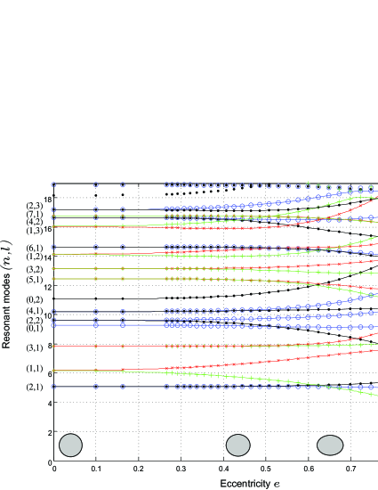
Figure 4: Tracking of the $k$-resonances versus the eccentricity $e$: ($\circ,A_{1}$) ; ($\cdot,A_{2}$) ; $(\times,B_{1})$ ; $(+,B_{2})$.

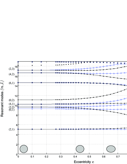
Figure 5: Splitting $(\times,A_{1})$ ; $(+,A_{2})$, even angular index $n.$

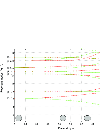
Figure 6: Splitting $(\times,B_{1})$ ; $(+,B_{2})$, odd angular index $n.$

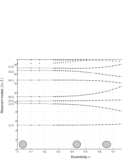
Figure 7: Mode interaction.

3.2 Vibrational normal modes displacement

The elastic displacement associated with each irreducible representation $R_{i}$ permits to compute the vibrational normal modes displacement. We plot $\left|\mathbf{u}^{R_{i}}\right|$ for various eccentricities. This computation requires the evaluation of the unknown coefficients to determine the fields $\phi$ and $\psi$ involved in (7jmopsuwxzaaacadag). These coefficients are calculated by solving the systems of equations (7jmopsua-7jmopsub), (7jmopsuwxa-7jmopsuwxb), (7jmopsuwxzaaa-7jmopsuwxzaab) and (7jmopsuwxzaaacada-7jmopsuwxzaaacadb). In the case of circular disc, for a given degenerated mode, the transition from a representation to an other can be done by a simple rotation of an angle $\pi/2n$ (see figure 8 for $b/a=1$). Once the circular disc is deformed into the elliptical one, the symmetry is broken and patterns become quite different. Mode splittings are observed as the eccentricity increases (figure 8). Only group theory permits one to highlight the splitting up and to link the splitted modes with the initial degenerated mode of the circular disc.

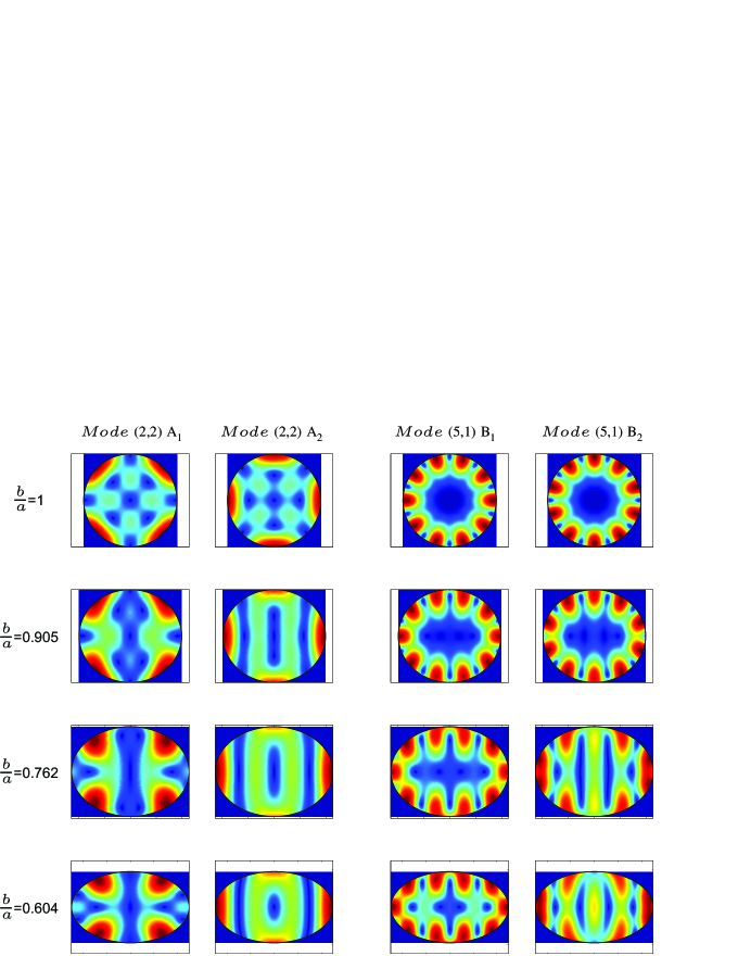
Figure 8: Vibrational normal modes displacement.

3.3 Periodic orbits

In order to give a physical interpretation in terms of trajectories, we use periodic orbits theory [20, 21]. We numerically compute the spectral counting function

$$\mathcal{N}(k)=\sum_{n}\Theta(k-k_{n})$$ (7jmopsuwxzaaacadagah)

giving the number of the $k$-resonances. The equation (7jmopsuwxzaaacadagah) can be quite generally written in terms of a smooth part and an oscillating part, the latter containing the periodic orbits contribution, that is

$$\mathcal{N}(k)=\mathcal{N}_{\mathit{smooth}}(k)+\mathcal{N}_{\mathit{oscill}}(k).$$ (7jmopsuwxzaaacadagai)

General results for the smooth part of the counting function of isotropic elastic media with free boundary conditions can be found in [22, 23]. The decomposition (7jmopsuwxzaaacadagai) gives an explicit connection between periodic ray trajectories in the elliptical disc and the eigenfrequencies of the system. By taking the Fourier transform of $\mathcal{N}_{\mathit{oscill}}(k)$, one should be able to recover the periodic trajectories including orbits that change polarization along their path.

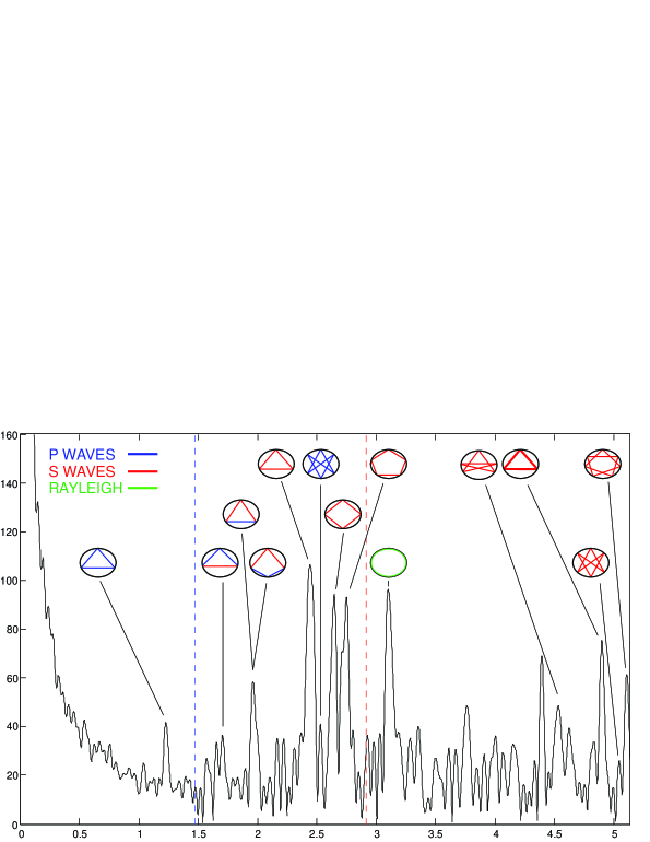
Figure 9: Periodic orbits spectrum of an aluminium elliptical disc $e=0.6$ ($\frac{b}{a}=0.8$).

Figure 9 shows a numerically calculated period spectrum obtained from the first $1540$ resonances of an aluminium elliptical disc (Ag4mc - $c_{L}=6344.8$ m.s^-1, $c_{T}=3196$ m.s^-1) in the frequency range $0<k\leq 150$. We remove the smooth part of $\mathcal{N}(k)$ and take the Fourier transform. The thus obtained period spectrum shows numerous peaks that correspond to: orbits being of pure pressure, pure shear, mixed polarization types, and pure Rayleigh orbit. The two dashed lines correspond to accumulation towards a limit orbit when segments of pure pressure or pure shear become tangential to the boundary. For example, orbits such as the irregular pentagram or those that turn twice (appearing at $\approx 4.9$) can also be resolved. We note that orbits with segments of both pressure and shear polarization type arise when mode conversion occurs. Surface Rayleigh orbit (appearing at $\approx 3.1$) can also be clearly identified including in spectra computed for other various eccentricities. The lengths of periodic orbits of pure pressure and pure shear are obtained using the expressions given by Sieber [24], whereas those undergoing mode conversion are geometrically obtained using Snell-Descartes law. The abscissa axis actually corresponds to dimensionless travel time due to the chosen frequency normalization.

4 Conclusion and perspectives

From symmetry considerations, a classification of resonances of the elastic elliptical disc has been provided: they lie in four distinct families associated with the four irreducible representations $A_{1},A_{2},B_{1},B_{2}$ of the symmetry group $\mathcal{C}_{2v}$ of the elliptical disc. Each resonant mode is labelled by the two numbers $\left(n,\ell\right)$ in the modal formalism associated to the circular disc. They are also tagged by the associated irreducible representation. The splitting up of resonances is emphasized and algebraic considerations permit to understand this phenomenon. This method significantly simplifies the numerical treatment of the problem. The computations can be also carried out in case of large eccentricities when rapid variations of the curvature radius occur.

A connection between the resonances spectrum and the periodic orbits spectrum is established. Due to mode conversion, orbits changing polarization along their path appear. The pure Rayleigh orbit is also clearly resolved for various eccentricities.

Finally, a series of experiments will be added to the theoretical studies. An experimental part based on laser impacts excitation and laser vibrometry will be carried out for three-dimensional objects. We expect to observe splitting up of resonances and resonant modes crossings when the sphere is deformed to the spheroid (symmetry breaking $\mathcal{O}(3)$ $\rightarrow$ $\mathcal{D}_{\infty h}$), as we theoretically observe in the two-dimensional case when the circular disc is deformed to the elliptical one.

The method described in this paper is also well suited to scattering problems such as acoustic scattering by infinite elastic cylinders of elliptical cross-section (work in preparation). In this context, further experiments in underwater acoustic scattering will also be performed.

Appendix A Coefficients

The structural functions involving Bessel functions are angular dependent. They are given by

$$c_{q}^{L} = (x_{T}^{2}-2q^{2})J_{q}(x_{L})+2x_{L}J_{q}^{\prime}(x_{L})$$ (7jmopsuwxzaaacadagaj)

$$d_{q}^{L} = 2q(x_{L}J_{q}^{\prime}(x_{L})-J_{q}(x_{L}))$$ (7jmopsuwxzaaacadagak)

$$c_{q}^{T} = f_{q}^{T}=2q(x_{T}J_{q}^{\prime}(x_{T})-J_{q}(x_{T}))$$ (7jmopsuwxzaaacadagal)

$$d_{q}^{T} = (x_{T}^{2}-2q^{2})J_{q}(x_{T})+2x_{T}J_{q}^{\prime}(x_{T})$$ (7jmopsuwxzaaacadagam)

$$f_{q}^{L} = (2x_{L}^{2}-x_{T}^{2}-2q^{2})J_{q}(x_{L})+2x_{L}J_{q}^{\prime}(x_{L})$$ (7jmopsuwxzaaacadagan)

where $x_{j}=k_{j}r(\theta)$, $j\in\{L,T\}$, $q\in\mathbb{N}$ (even or odd).

Appendix B Fourier coefficients

The Fourier coefficients are evaluated on the restricted fundamental domain, they are numerically calculated from the following expressions

$$\beta_{q,r}^{j} = \frac{2}{\pi}\int_{0}^{\frac{\pi}{2}}[c_{q}^{j}\cos(q\theta)\;n_{\rho}+d_{q}^{j}\sin(q\theta)\;n_{\theta}]\cos(r\theta)d\theta$$ (7jmopsuwxzaaacadagao)

$$\xi_{q,r}^{j} = -\frac{2i}{\pi}\int_{0}^{\frac{\pi}{2}}[d_{q}^{j}\sin(q\theta)\;n_{\rho}-f_{q}^{j}\cos(q\theta)\;n_{\theta}]\sin(r\theta)d\theta$$ (7jmopsuwxzaaacadagap)

$$\alpha_{q,r}^{L} = -\frac{2i}{\pi}\int_{0}^{\frac{\pi}{2}}[c_{q}^{L}\sin(q\theta)\;n_{\rho}-d_{q}^{L}\cos(q\theta)\;n_{\theta}]\sin(r\theta)d\theta$$ (7jmopsuwxzaaacadagaq)

$$\alpha_{q,r}^{T} = -\frac{2i}{\pi}\int_{0}^{\frac{\pi}{2}}[-c_{q}^{T}\sin(q\theta)\;n_{\rho}+d_{q}^{T}\cos(q\theta)\;n_{\theta}]\sin(r\theta)d\theta$$ (7jmopsuwxzaaacadagar)

$$\eta_{q,r}^{L} = \frac{2}{\pi}\int_{0}^{\frac{\pi}{2}}[-d_{2n}^{L}\cos(q\theta)\;n_{\rho}-f_{q}^{L}\sin(q\theta)\;n_{\theta}]\cos(r\theta)d\theta$$ (7jmopsuwxzaaacadagas)

$$\eta_{q,r}^{T} = \frac{2}{\pi}\int_{0}^{\frac{\pi}{2}}[d_{q}^{T}\cos(q\theta)\;n_{\rho}+f_{q}^{T}\sin(q\theta)\;n_{\theta}]\cos(r\theta)d\theta$$ (7jmopsuwxzaaacadagat)

$j\in\{L,T\}$, $\left(q,r\right)\in\mathbb{N}^{2}$ (even or odd).

References

References

• [1] A. E. H. Love. A treatise on the mathematical theory of elasticity. Dover Books on Engineering, 1906.
• [2] H. Lamb. On the vibrations of an elastic sphere. In Proc. London Math. Soc., volume 13, pages 51–66. London Mathematical Society, 1882.
• [3] W. M. Visscher, A. Migliori, T. M. Bell, and R. A. Reiner. On the normal modes of free vibration of inhomogeneous and anisotropic elastic objects. J. Acoust. Soc. Am., 90(4):2154–2162, 1991.
• [4] L. Saviot and D. B. Murray. Longitudinal versus transverse spheroidal vibrational modes of an elastic sphere. Phys. Rev B, 72(20):205433.1–205433.6, 2005.
• [5] G. Tanner and N. Søndergaard. Wave chaos in the elastic disk. Phys. Rev. E, 66(066211), 2002.
• [6] J. J. Bowman, T. B. A. Senior, P. L. E. Uslenghi, and J. S. Asvestas. Electromagnetic and acoustic scattering by simple shapes. North-Holland Pub. Co., 1970.
• [7] V. V. Varadan and Y. H. Pao. Scattering matrix for elastic waves. i. theory. J. Acoust. Soc. Am., 60(3), September 1976.
• [8] F. Léon, F. Chati, and J. M. Conoir. Modal theory applied to the acoustic scattering by elastic cylinders of arbitrary cross section. J. Acoust. Soc. Am., 116(2), 2004.
• [9] F. P. Mechel. Mathieu functions: formulas, generation, use. S. Hirzel Verlag Stuttgart, 1997.
• [10] S. Ancey, A. Folacci, and P. Gabrielli. Whispering-gallery modes and resonances of an elliptic cavity. J. Phys. A: Math. Gen., 34:2657, 2001.
• [11] V. V. Varadan. Scattering matrix for elastic waves. ii. application to elliptic cylinders. J. Acoust. Soc. Am., 63(4), Apr. 1978.
• [12] A. Wirzba, N. Søndergaard, and P. Cvitanović. Wave chaos in elastodynamic cavity scattering. Europhys. Lett., 72(4):534, 2005.
• [13] Y. Decanini, A. Folacci, P. Gabrielli, and J. L. Rossi. Algebraic aspects of multiple scattering by two parallel cylinders: classification and physical interpretation of scattering resonances. Journal of Sound and Vibration, 221:785–804, 1999.
• [14] P. Gabrielli and M. Mercier-Finidori. Acoustic scattering by two spheres: multiple scattering and symmetry considerations. Journal of Sound and Vibration, 241(3):423–439, 2001.
• [15] P. J. Moser and H. Überall. Complex eigenfrequencies of axisymmetric, perfectly conducting bodies: Radar spectroscopy. In Proc. IA, volume 71, pages 171–172. IEEE, 1983.
• [16] P. A. Chinnery and V. F. Humphrey. Fluid column resonances of water-filled cylindrical shells of elliptical cross section. J. Acoust. Soc. Am., 103(3), March 1998.
• [17] S. Ancey. Résonances en géométrie elliptique: développements asymptotiques exponentiellement améliorés et levée de dégénérescence. PhD thesis, Université de Corse - Pascal Paoli, 2000.
• [18] M. Hamermesh. Group Theory and its Application to Physical Problems. New York: Dover, 1989.
• [19] L. Landau and E. Lifchitz. Physique théorique, tome 7. Théorie de l’élasticité. Librairie du Globe, ed. MIR, 1990.
• [20] M. V. Berry and M. Tabor. Closed orbits and the regular bound spectrum. In Proceedings of the Royal Society A, number 349, pages 101–123. Royal Society, 1976.
• [21] M. V. Berry and M. Tabor. Calculating the bound spectrum by path summation in action- angle variables. J. Phys. A: Math. Gen., 10(3), 1977.
• [22] M. Dupuis, R. Mazo, and L. Onsager. Surface specific heat of an isotropic solid at low temperatures. J. Chem. Phys., 33(5), 1960.
• [23] Y. Safarov and D. G. Vasil’ev. Spectral theory of operators (American Mathematical Society Translations vol 150). ed. S Gindikin (Princeton, NJ: American Mathematical Society), 1992.
• [24] M. Sieber. Semiclassical transition from an elliptical to an oval billiard. J. Phys. A: Math. Gen., 30:4563–4596, 1997.