Trajectory control of a bipedal walking robot with inertial disc

Abstract

In this paper we exploit some interesting properties of a class of bipedal robots which have an inertial disc. One of this properties is the ability to control every position and speed except for the disc position. The proposed control is designed in two hierarchic levels. The first will drive the robot geometry, while the second will control the speed and also the angular momentum. The exponential stability of this approach is proved around some neighborhood of the nominal trajectory defining the geometry of the step. This control will not spend energy to adjust the disc position and neither to synchronize the trajectory with the time. The proposed control only takes action to correct the essential aspects of the walking gait. Computational simulations are presented for different conditions, serving as a empirical test for the neighborhood of attraction.

1 Introduction

Dynamic robot locomotion is a particularly challenging study. One of its main difficulties is due to the fact that the robot is sub-actuated, that is, on a dynamic walking gait it is impossible to freely control each orientation of the robot’s links. It is straightforward to see this limitation as there is no actuator between the ground and the support polygon, the gravity alone will impose an additional torque that will change the robot orientation. Aside from this, a dynamic walking bipedal robot can achieve greater speeds than a static walker, so there is a practical interest in this domain of research.

In Westervelt et al. (2007) the problem of sub-actuated dynamic walking is treated in a systematic way that will lead to controller design with assured stability and also, with a step evolution clocked, not by the time, but by its own geometry. This self clocked characteristic will be instrumental in this work. We can see each step as a trajectory for the state vector of the dynamic model. The classical controller design will ensure the state of the model to track some reference tied to the time and some control effort will take place even if the robot state is valid for the reference trajectory but is not synchronized with the reference.

To successfully perform a step, the robot links must be driven in some specific way, even for coordinates that cannot be directly controlled. To accomplish this it may be necessary, for example, to swing the robot’s torso and this can be undesirable in some cases.

To have complete control over one coordinate, it is necessary to give up the control of another one. So, if it is possible to ignore the position or the orientation of a link, it will be possible to control every other important coordinate. By using a inertial disc, its orientation will be a cyclic variable, and thus, could be ignored. That is the main idea introduced by the design presented in Kieffer and Bale (1993) and studied in many works as Rouchon and Sira-Ramirez (2003), Spong et al. (2000) and Peres (2008). Theoretically it is possible to ignore the disc position and speed, but in practice, there will be some limitation on the maximum speed achieved by the disc, so that the actuators do not saturate. One solution to this problem is proposed in Peres (2008) by means of a supervisory control, that will perform a different trajectory if the disc speed is beyond some limit value.

Section 2 presents the hybrid dynamic model as proposed in Westervelt et al. (2007). There is also a brief presentation of the hypotheses and terminology therein and inherited by this paper.

Next, it will be introduced the trajectory planning in section 3. This is the main practical benefit of our approach, valid only for this specific class of bipedal robots. In Westervelt et al. (2007), the proposed strategy is to find the evolution of the robot geometry as function of the absolute orientation and then check if it will lead to a monotonic evolution of that absolute orientation. In our approach, it is possible to fix the robot geometry as a desired function of the absolute orientation. Then find a monotonic evolution of the absolute orientation that lead to a repeatable evolution of the disc speed. Another benefit is that the proposed control does not deal at all with the disc position, but can continuously control its speed. The control law and the convenient change of coordinates is also presented, introducing the core contribution of this paper.

Section 4 present a demonstration of exponential stability around some neighborhood of the planed trajectory.

Finally in section 5 there are some simulation results.

2 Dynamic Model

The robot will be modeled by a chain of $N$ rigid links, each one with known parameters such as mass, center of mass and inertia. The links are connected by $N-1$ frictionless joints independently actuated. There will be at least one and at most two point of contact with the ground, called foots. The foots are punctual and unactuated.

For illustration purposes, a very simple bipedal robot is depicted at figure 1. The coordinate $q_{N}$ is the only absolute coordinate, $q_{d}$ is a relative coordinate to represent the disc position and $\mathbf{q}_{r}$ is a relative coordinate representing the angular displacement between the two legs.

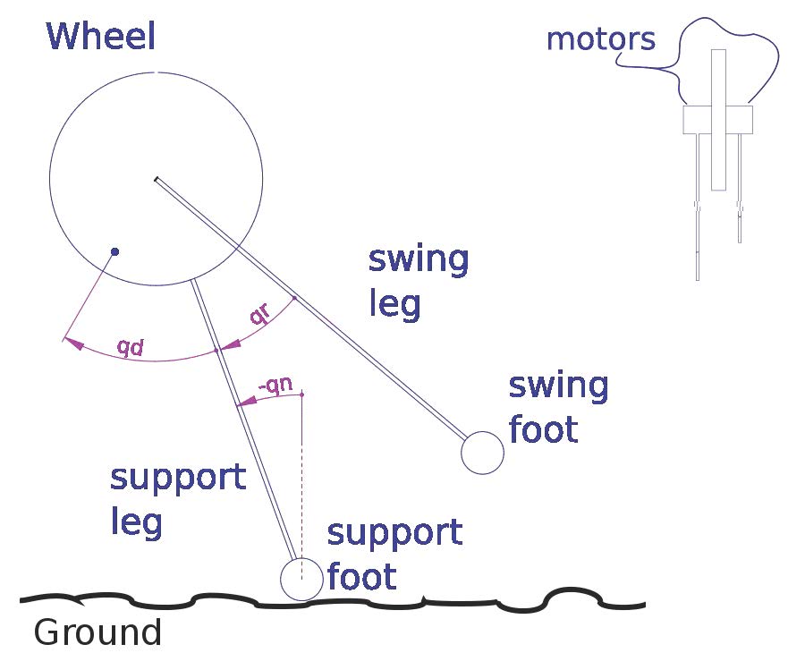
Figure 1: Example model. Side view with coordinates and detail of frontal view in the upper right corner.

On a higher order robots $\mathbf{q}_{r}$ will be a vector representing the angular displacements between each link. Indeed, the robot’s shape will be determined by $\mathbf{q}_{r}$.

The walking takes place on a surface, is restricted to the sagittal plane, and is composed of alternating phases of single and double support. During the single support phase, the stance foot acts as an ideal pivot. The double support phase is instantaneous and associated impacts are modeled as a rigid contact. At the impact, the swing leg touches the ground with no slip nor rebound and, the former stance leg releases without interaction.

The robot model is derived under the hypotheses briefly cited above and detailed in Westervelt et al. (2007), HR1~HR5, HGW1~HGW7 and HI1~HI7 ((Westervelt et al., 2007, p48 p50)). A small change is introduced in HR6.

• the model is expressed in one relative coordinate $q_{d}$ for the disc, N-2 relative coordinates $\mathbf{q}_{r}$ for the rest of the body and only one absolute coordinate $q_{N}$.

Using Lagrangian formulation, the dynamic equations for the continuous phase, between two impacts, will be

$$\mathbf{D}\left(\mathbf{q}_{r}\right)\mathbf{\ddot{q}}+\mathbf{C}\left(\mathbf{q}_{r},\mathbf{\dot{q}}_{r},\dot{q}_{N}\right)\dot{\mathbf{q}}+\mathbf{G}\left(\mathbf{q}_{r},q_{N}\right) = \mathbf{B}\left(\mathbf{q}_{r}\right)\mathbf{u}$$ (1)

where

$$\mathbf{q} \triangleq \left(\begin{array}[]{ccc}q_{d}&\mathbf{q}_{r}&q_{N}\end{array}\right)^{T}$$ (3)

$q_{d}\in\mathbb{R}$, $\mathbf{q}_{r}\in\mathbb{R}^{N-2}$, $q_{N}\in\mathbb{R}$ and the vector of actuator torques being defined by $\mathbf{u}\in\mathbb{R}^{N-1}$. $\mathbf{D}\left(\mathbf{q}_{r}\right)$ is called the Inertia Matrix, $\mathbf{C}\left(\mathbf{q}_{r},\dot{\mathbf{q}}_{r}\right)$ is called the Coriolis Matrix, $\mathbf{G}\left(\mathbf{q}_{r},q_{N}\right)$ is called the Gravity Vector and $\mathbf{B}\left(\mathbf{q}_{r}\right)$ will map the actuator torques as generalized forces.

It will be more convenient to define

$$\omega \triangleq \left(\begin{array}[]{ccc}\sigma_{N}&\dot{\mathbf{q}}_{r}&\dot{q}_{N}\end{array}\right)^{T}$$ (5)

where $\sigma_{N}$ is the angular moment of the system, calculated as

$$\sigma_{N} = \mathbf{D}_{N}\left(\mathbf{q}_{r}\right)\dot{\mathbf{q}}$$ (6)

$\mathbf{D}_{N}$ being the last line of the inertia matrix. Its derivative will be

$$\dot{\sigma}_{N} = -\mathbf{G}_{N}\left(\mathbf{q}_{r},q_{N}\right)$$ (7)

$\mathbf{G}_{N}$ being the last line of the gravity vector.

There will be a diffeomorphism between $\dot{\mathbf{q}}$ and $\omega$ and so it is possible to define the state vector

$$\mathbf{x} \triangleq \left(\begin{array}[]{cc}\mathbf{q}&\omega\end{array}\right)^{T}$$ (9)

and denote by $\mathcal{X}\subset\mathbb{R}^{N}$ the set of valid values for the vector state $\mathbf{x}$.

At some moment, the swing foot will touch the ground with state $\mathbf{x}^{-}$ and the system will be mapped to a new state $\mathbf{x}^{+}$. It is assumed that the walking gait is transversal to the impact surface. So, the impact forces will change the speeds on $\omega$. After the impact the roles of the legs are reversed with a change in $\mathbf{q}$. As result, the system state, $\mathbf{x}^{+}$, after the impact is

$$\mathbf{x}^{+} = \Delta\left(\mathbf{x}^{-}\right)$$ (10)

$$\Delta = \left(\begin{array}[]{c}\Delta_{\mathbf{q}}\mathbf{q}_{s}^{-}\\ \Delta_{\omega}\left(\mathbf{q}_{r}^{-},q_{N}^{-}\right)\omega^{-}\end{array}\right)$$ (13)

with $\Delta_{\mathbf{q}}$ being a constant involutive matrix and $\Delta_{\omega}$ a function of the robot geometry $\mathbf{q}_{r}^{-}$ and absolute orientation $q_{N}^{-}$. Note that any value with a superscript $\mathbf{q}^{-}$ means the value just before the impact at the end of the step, and a superscript $\mathbf{q}^{+}$ means the value immediately after the impact at the beginning of a new step. This is the same notation utilized in Westervelt et al. (2007).

The impact, modeled by the mapping $\Delta\left(\mathbf{x}^{-}\right)$, will take place at a given configuration that can be represented by a manifold $\mathcal{S}$, for example

$$\mathcal{S} \triangleq \left\{\mathbf{x}\in\mathcal{X}|p_{2}\left(\mathbf{q}\right)=0,\dot{p}_{2}\left(\mathbf{x}\right)<0\right\}$$ (14)

where $p_{2}\left(\mathbf{q}\right)\geq 0$ is a convenient function for which $\dot{p}_{2}\left(\mathbf{x}^{+}\right)>0$ and $\dot{p}_{2}\left(\mathbf{x}^{-}\right)<0$. The complete hybrid model will be

$$\begin{cases}\dot{\mathbf{x}}=\mathbf{f}\left(\mathbf{x}\right)+\mathbf{g}\left(\mathbf{x}\right)\mathbf{u}&\mathbf{x}\notin\mathcal{S}\\ \mathbf{x}^{+}=\Delta\left(\mathbf{x}^{-}\right)&\mathbf{x}\in\mathcal{S}\end{cases}$$ (15)

For this particular class of robots, if the coordinate vector is choose as (9) then it is possible to demonstrate that the first column of $\Delta_{\omega}$ is always $\left(\begin{array}[]{cccc}1&0&\cdots&0\end{array}\right)^{T}$. This is due to $q_{d}$ being a cyclic coordinate.

3 Design of the trajectory

In this section we present some aspects of the trajectory generation.

3.1 Ensuring a geometry tied to the absolute orientation

The idea of a geometry tied to the absolute orientation is presented in Westervelt et al. (2007). In this kind of design, all the actuators will be used to drive the robot geometry as a function of the absolute orientation. This geometry must be chosen in a way that, apart from not being directly controlled, the absolute orientation will have a monotonic evolution. Also, the interaction of the robot with the ground must produce a stable limit cycle.

In our robot, the disc position will be ignored. This allows us to get a new input available. Every relative link orientation, except for the disc coordinate $q_{d}$, should track a predefined function of $q_{N}$. This way, at any time, the robot configuration will be a function of its absolute orientation. This kind of control is equivalent to drive $\mathbf{q}_{r}-\mathbf{h}_{r}^{ref}\left(q_{N}\right)$ to zero on the output defined as

$$\mathbf{h} = \left(\begin{array}[]{cc}\mathbf{h}_{r}&q_{N}\end{array}\right)^{T}$$ (17)

$$\mathbf{h}_{r} = \mathbf{q}_{r}-\mathbf{h}_{r}^{ref}\left(q_{N}\right)$$ (18)

with $\mathbf{h}_{r}^{ref}\left(q_{N}\right)$ being the desired evolution of $\mathbf{q}_{r}$ as a function of $\mathbf{q}_{N}$. The output described by (17) has dimension $N-1$ which is the same dimension of the input $\mathbf{u}$. The dynamic system can be written in terms of the global diffeomorphism defined by

$$\mathbf{p} = \left(\mathbf{h},q_{d},\dot{\mathbf{h}},\sigma_{N}\right)$$ (19)

If the decoupling matrix $\mathcal{L}_{g}\mathcal{L}_{f}\mathbf{h}$ is square and invertible, there exists a input

$$\mathbf{u}^{*} = \left(\mathcal{L}_{g}\mathcal{L}_{f}\mathbf{h}\right)^{-1}\left\{\mathbf{v}-\mathcal{L}_{f}^{2}\mathbf{h}\right\}$$ (20)

so that by the use of $\mathbf{u}^{*}$ and the coordinate change (19), the system can be viewed as $N-1$ independent series of 2 integrators driven by the virtual input $\mathbf{v}=\left(\mathbf{v}_{r},v_{N}\right)^{T}$.

Thus, if it is possible to find $\mathbf{u}^{*}$, it will be possible to control every entry of $\mathbf{h}$ by the input $\mathbf{v}$. More information on the exact linearization control can be found in Isidori (1995).

Applying the change of coordinates defined by (19) it is possible to write

$$\dot{\sigma}_{N} = k_{2}\left(\mathbf{h}_{r},q_{N}\right)$$ (21)

$$k_{2}\left(\mathbf{h}_{r},q_{N}\right) \triangleq -\mathbf{G}_{N}\left(\mathbf{h}_{r}+\mathbf{h}_{r}^{ref}\left(q_{N}\right),q_{N}\right)$$ (22)

Using the input (20), the change of coordinates (19) and discarding $q_{d}$, it is possible to rewrite the continuous phase as

$$\cfrac{d}{dt}\left(\begin{array}[]{c}h_{r}\\ \dot{h}_{r}\\ \sigma_{N}\\ q_{N}\\ \dot{q}_{N}\end{array}\right) = \left(\begin{array}[]{c}\dot{h}_{r}\\ 0\\ k_{2}\left(\mathbf{h}_{r},q_{N}\right)\\ \dot{q}_{N}\\ 0\end{array}\right)+\left(\begin{array}[]{c}0\\ \mathbf{v}_{r}\\ 0\\ 0\\ v_{N}\end{array}\right)$$ (38)

Now define an embedded manifold

$$\mathcal{W} \triangleq \left\{\mathbf{x}\in\mathcal{X}|h_{r}=0,\,\dot{h}_{r}=0\right\}$$ (39)

From equation (38) it is possible to see that the input $\mathbf{v}_{r}$ can be used to drive $\mathbf{h}_{r}=0$. The input $v_{N}$ remains free to control the absolute speed $\dot{q}_{N}$ and also, when restricted to $\mathcal{W}$, the angular momentum $\sigma_{N}$.

Assume that it is possible to find functions $V\left(q_{N}\right)>0$ and $S\left(q_{N}\right)$, such that if $\dot{q}_{N}=V\left(q_{N}\right)$, then $\sigma_{N}=S\left(q_{N}\right)+\mathbb{C}_{\sigma}$, where $\mathbb{C}_{\sigma}$ is some constant bias. It is possible to use the input $v_{N}$ to exponentially attenuate this bias.

3.2 Finding a periodic step

The manifold $\mathcal{W}$ is said to be forward invariant if solutions starting at $\mathcal{W}$ will remain in $\mathcal{W}$. It will be said to be impact invariant if $\mathcal{W}\cap\mathcal{S}\neq\emptyset$ and $\Delta\left(\mathcal{W}\cap\mathcal{S}\right)\subset\mathcal{W}$. Observe that $\Delta\left(\mathcal{W}\cap\mathcal{S}\right)\cap\mathcal{S}=\emptyset$. If $\mathcal{W}$ is both forward and impact invariant, it is said to be hybrid invariant (Westervelt et al., 2007, p 96). While the feedback control can lead to forward invariance, the impact invariance is a design property.

For the nominal trajectory to be repeated, each variable evolution must be hybrid invariant. So, not only $\mathcal{W}$, but also the angular momentum reference $S\left(q_{N}\right)$, and the absolute speed reference $V\left(q_{N}\right)$, has to be hybrid invariant themselves.

One procedure to find such nominal trajectory would be:

1. Fix the absolute orientations at the beginning, $q_{N}=\bar{q}_{N}^{+}$, and at the end, $q_{N}=\bar{q}_{N}^{-}$, of the step, and the nominal configurations $\bar{\mathbf{q}}^{+}$ and $\bar{\mathbf{q}}^{-}$.

2. Determine a desirable evolution $\mathbf{h}_{r}^{ref}\left(q_{N}\right)$ for the robot configuration, such that

   1. $\bar{\mathbf{q}}^{+}=\Delta_{\mathbf{q}}\bar{\mathbf{q}}^{-}\forall\mathbf{q}\in\mathcal{W}$, as $q_{d}$ is a cyclic coordinate, it can be ignored; this will ensure impact invariance on the robot shape $\mathbf{h}_{r}^{ref}\left(q_{N}\right)$

   2. depending on the value of $\Delta_{\omega}\left(\bar{\mathbf{q}}_{r}^{-},\bar{q}_{N}^{-}\right)$, determine $\cfrac{\partial\mathbf{h}_{r}^{ref}\left(q_{N}^{+}\right)}{\partial q_{N}}$ and $\cfrac{\partial\mathbf{h}_{r}^{ref}\left(q_{N}^{-}\right)}{\partial q_{N}}$ for impact invariance of $\dot{\mathbf{h}}_{r}^{ref}\left(q_{N}\right)$. There will be also a fixed increment or decrement of the angular momentum $\Delta_{\sigma}=\sigma_{N}^{-}-\sigma_{N}^{+}$. This will lead to impact invariance on $\mathcal{W}$.

3. choose a impact invariant and convenient function candidate for $V\left(q_{N}\right)>0$ , then numerically calculate

   $$S\left(q_{N}\right) = \intop_{q_{N}^{+}}^{q_{N}}\tfrac{k_{2}\left(0,\tau\right)}{V\left(\tau\right)}d\tau+\sigma_{N}^{+}$$ (40)

   such that $\Delta_{\sigma}=S\left(q_{N}^{-}\right)-S\left(q_{N}^{+}\right)$ will satisfy the impact invariance restriction for $S\left(q_{N}\right)$.

The control must ensure forward invariance and also a stability around this planned trajectory.

3.3 A new change of coordinates

By construction of $V\left(q_{N}\right)$ and $S\left(q_{N}\right)$, when restricted to $\mathcal{W}$, where $\mathbf{h}_{r}=\mathbf{0}$, the following relation holds

$$\left.k_{2}\left(q_{N},\mathbf{h}_{r}\right)\right|_{\mathcal{W}} = \cfrac{\partial S\left(q_{N}\right)}{\partial q_{N}}V\left(q_{N}\right)$$ (41)

and so it is possible to write

$$k_{2}\left(\mathbf{h}_{r},q_{N}\right)-\cfrac{\partial S\left(q_{N}\right)}{\partial q_{N}}V\left(q_{N}\right) = \left\langle\mathbf{h}_{r},\mathbf{f}_{2}\left(\mathbf{h}_{r},q_{N}\right)\right\rangle$$ (42)

where $\mathbf{f}_{2}\left(\mathbf{h}_{r},q_{N}\right)$ is a unknown but bounded function.

Suppose now that exist hybrid impact invariant functions $\mathbf{h}_{r}^{ref}\left(q_{N}\right)$, $V\left(q_{N}\right)$ and $S\left(q_{N}\right)$ . Then if we choose

$$\mathbf{v}_{r} = -K_{P}\mathbf{h}_{r}-K_{V}\mathcal{L}_{f}\mathbf{h}_{r}$$ (43)

with $K_{P}$ and $K_{V}$ positive definite, this will ensure convergence of $\mathbf{q}_{r}\rightarrow\mathbf{h}_{r}^{ref}\left(q_{N}\right)$. The convergence $\mathbf{x}\rightarrow\mathcal{W}$ will be independent of $q_{N}$, $\dot{q}_{N}$, $q_{d}$ or $\dot{q}_{d}$ and also $\mathcal{W}$ will be forward invariant.

The input $v_{N}$ can be freely used to drive the absolute orientation of the robot. It is theoretically possible to track any reference trajectory by the use of the output (17) as we found a linearizable part of dimension $2N-2$, the side effect being that we do not have direct control over the speed accumulated by the disc. But there is an interesting property of this robot, as $q_{d}$ and $\dot{q}_{d}$ can be ignored for the dynamic model. So the remaining coordinates will be $q_{r}$, $q_{N}$ , $\sigma_{N}$, $\dot{q}_{r}$, $\dot{q}_{N}$. As $q_{N}$ is the only absolute coordinate, $\mathbf{D}$ is also independent of $q_{N}$.

Now define

$$b \triangleq \sigma_{N}-S\left(q_{N}\right)$$ (44a)

$$c \triangleq \dot{q}_{N}-V\left(q_{N}\right)-\cfrac{\gamma}{\beta_{0}}\cfrac{\partial S\left(q_{N}\right)}{\partial q_{N}}b$$ (44b)

with $\gamma$ and $\beta_{0}$ positive constants. It is possible to define the manifold

$$\mathcal{Z} \triangleq \left\{\mathbf{x}\in\mathcal{W}|b=0,c=0\right\}$$ (45)

and it will be impact invariant. When the robot is performing the nominal step, $\mathbf{x}\in\mathcal{Z}$ and $\mathcal{Z}\cap\mathcal{S}\in\mathbb{R}$.

As $q_{N}$ is monotonic at the continuous phase, it is possible to integrate (38) at $q_{N}$ and rewrite it using the coordinates

$$\mathbf{y} \triangleq \left(\begin{array}[]{cccc}\mathbf{h}_{r}&\dot{\mathbf{h}}_{r}&b&c\end{array}\right)^{T}$$ (47)

So, defining

$$\xi\left(q_{N}\right) \triangleq \left(c\left(q_{N}\right)+V\left(q_{N}\right)+\nicefrac{{\gamma}}{{\beta_{0}}}\cfrac{\partial S}{\partial q_{N}}b\left(q_{N}\right)\right)^{-1}$$ (48)

using the input $\mathbf{v}_{r}$ as defined in (43) and $v_{N}$ as

$$v_{N} = \cfrac{\partial V}{\partial q_{N}}\dot{q}_{N}+\gamma\cfrac{\partial S}{\partial q_{N}}b-\beta_{0}\left(\dot{q}_{N}-V\right)+\cfrac{d}{dt}\left(\cfrac{\gamma}{\beta_{0}}\cfrac{\partial S}{\partial q_{N}}b\right)$$ (49)

then the continuous part of the dynamic system, subject to the given hypotheses, can be written as

$$\cfrac{d\mathbf{y}}{dq_{N}} = \bar{\mathbf{f}}\left(\mathbf{y},q_{N}\right)$$ (50)

$$\bar{\mathbf{f}}\left(\mathbf{y},q_{N}\right) \triangleq \xi\left(\begin{array}[]{c}\dot{\mathbf{h}}_{r}\\ -K_{P}\mathbf{h}_{r}-K_{V}\dot{\mathbf{h}}_{r}\\ \left\langle\mathbf{h}_{r},\mathbf{f}_{2}\right\rangle-\tfrac{\partial S}{\partial q_{N}}c-\nicefrac{{\gamma}}{{\beta_{0}}}\left(\tfrac{\partial S}{\partial q_{N}}\right)^{2}b\\ -\beta_{0}c\end{array}\right)$$ (55)

Note also that by using the input (49), the impact invariant manifold $\mathcal{Z}$ will be forward invariant and thus, hybrid invariant.

In this new coordinates, the impact map will be

$$\left(\begin{array}[]{c}q_{d}^{+}\\ \mathbf{h}_{r}^{+}\\ q_{N}^{+}\end{array}\right) = \Delta_{q}\left(\begin{array}[]{c}q_{d}^{-}\\ \mathbf{h}_{r}^{-}+\mathbf{h}_{r}^{ref}\left(q_{N}^{-}\right)\\ q_{N}^{-}\end{array}\right)-\left(\begin{array}[]{c}0\\ \mathbf{h}_{r}^{ref}\left(q_{N}^{+}\right)\\ 0\end{array}\right)$$ (56j)

$$\left(\begin{array}[]{c}b^{+}\\ \dot{\mathbf{h}}_{r}^{+}\\ c^{+}\end{array}\right) = \Delta_{p}\left(h_{r}^{-},q_{N}^{-},q_{N}^{+}\right)\left(\begin{array}[]{c}b^{-}\\ \dot{\mathbf{h}}_{r}^{-}\\ c^{-}\end{array}\right)$$ (56q)

where

$$\Delta_{p} = \Delta_{1}\left(q_{N}^{+}\right)\Delta_{\omega}\left(\mathbf{h}_{r}+\mathbf{h}_{r}^{ref}\left(q_{N}\right)\right)\Delta_{2}\left(q_{N}^{-}\right)$$ (57)

$$\Delta_{1} = \left(\begin{array}[]{ccc}1&0&0\\ 0&1&-\cfrac{\partial\mathbf{h}_{r}^{ref}}{\partial q_{N}}\\ -\nicefrac{{\gamma}}{{\beta_{0}}}\cfrac{\partial S}{\partial q_{N}}&0&1\end{array}\right)$$ (61)

$$\Delta_{2} = \left(\begin{array}[]{ccc}1&0&0\\ \nicefrac{{\gamma}}{{\beta_{0}}}\cfrac{\partial\mathbf{h}_{r}^{ref}}{\partial q_{N}}\cfrac{\partial S}{\partial q_{N}}&1&\cfrac{\partial\mathbf{h}_{r}^{ref}}{\partial q_{N}}\\ \nicefrac{{\gamma}}{{\beta_{0}}}\cfrac{\partial S}{\partial q_{N}}&0&1\end{array}\right)$$ (65)

From (56j) and (14) it is possible to find the impact effect over $\mathbf{h}_{r}$ and the actual integration limits $q_{N}^{+}$ and $q_{N}^{-}$, $q_{N}^{+}<q_{N}^{-}$. From (56q) it is possible to find how the remaining part of (47) are affected by the impact. The impact map with respect to the vector state (47) will be

$$\mathbf{y}^{+} = \Delta_{\mathbf{y}}\left(\mathbf{y}^{-}\right)$$ (66)

and can be obtained by reshaping (56) adequately. From (50) and (66), the complete hybrid system will be

$$\begin{cases}\cfrac{d\mathbf{y}}{dq_{N}}=\bar{\mathbf{f}}\left(\mathbf{y},q_{N}\right)&\mathbf{y}\notin\mathcal{S}\\ \mathbf{y}^{+}=\Delta_{y}\left(\mathbf{y}^{-}\right)&\mathbf{y}\in\mathcal{S}\end{cases}$$ (67)

3.4 Poincaré Map

When walking, the dynamic system (67) will take a periodic evolution composed of a continuous phase, followed by the impact map and another continuous phase. To evaluate the stability of this periodic orbit, it will be important to define Poincaré return map for the manifold $\mathcal{S}$ as

$$\mathcal{P} : \mathcal{S_{P}}\rightarrow\mathcal{S}$$ (68)

where $\mathcal{S_{P}}\in\mathcal{S}$ is a neighborhood of $\mathbf{y}=\mathbf{0}$, such that

$$\mathcal{P}\left(\mathbf{y}\right) \triangleq \varphi_{\mathbf{y}}\left(q_{N}^{+},q_{N}^{-},\Delta_{\mathbf{y}}\left(\mathbf{y}\right)\right)$$ (69)

with $\varphi_{\mathbf{y}}\left(q_{N}^{+},q_{N}^{-},\mathbf{y}_{0}\right)$ being the integral curve of (67) with initial condition $\mathbf{y}_{0}$, starting at $q_{N}=q_{N}^{+}$ and ending at $q_{N}=q_{N}^{-}$. So $\varphi_{\mathbf{y}}\left(q_{N}^{+},q_{N}^{+},\mathbf{y}_{0}\right)=\mathbf{y}_{0}$.

By the hybrid invariance of the manifold $\mathcal{Z}$, $\mathbf{y}_{0}=\mathbf{0}$ will be a fixed point of $\mathcal{P}$

$$\mathcal{P}\left(\mathbf{0}\right) = \mathbf{0}$$ (70)

As expected, there exist a periodic orbit of $\mathbf{y}\in\mathcal{Z}$ and, the interception of this periodic orbit with the impact surface $\mathcal{S}$, that is $\mathcal{S}\cap\mathcal{Z}$, occours at $\mathbf{y}=\mathbf{0}$.

4 Stability around the nominal step

Theorem 1

Under the given robot hypotheses and the existence of $\mathbf{h}_{r}^{ref}\left(q_{N}\right)$, $V\left(q_{N}\right)$ and $S\left(q_{N}\right)$ such that the manifolds $\mathcal{W}$ and $\mathcal{Z}$ are hybrid invariants, then:

- The Poincaré return map $\mathcal{P}$ is regular in some neighborhood $\mathcal{S_{P}}\subset\mathcal{S}$ around $\mathbf{y}=0$.

- The Poincaré return map $\mathcal{P}$ can be made locally exponentially contracting in some neighborhood $\mathcal{S_{C}}\subset\mathcal{S_{P}}$ of $\mathbf{y}=0$, by adjusting the parameters $K_{P}$, $K_{v}$, $\beta_{0}$ and $\gamma$.

Corollary 2

If it is possible to find (20) for every possible value of $\mathbf{x}$, then the the system (15), except for the disc position, can be made exponentially stable around some neighborhood $\mathcal{U}$ of $\mathcal{Z}$ by using the inputs defined by (43), (49) and adjusting the parameters $K_{P}$, $K_{v}$, $\beta_{0}$ and $\gamma$.

Proof 4.1

The Poincaré return map is well defined for $\mathbf{y}=\mathbf{0}$, $\mathcal{Z}\cap\mathcal{S}$, and this is its fixed point. The manifold $\mathcal{Z}$ is transversal to $\mathcal{S}$ and solutions of the hybrid system (67) are continuous. So for some sufficiently small perturbation $\epsilon\in\mathcal{S}$ around $\mathbf{0}$ before the impact, the continuous part of the system will reach again the impact surface. If $\mathcal{S_{P}}$ is defined to be the set in which, in the event of a impact, at least one another impact will follow, then it is possible to conclude that $\exists\mathcal{P}:\mathcal{S_{P}}\rightarrow\mathcal{S}$.

The impact map (57) can be linearized at $\mathcal{Z}\cap\mathcal{S}$. This will lead to

$$\mathbf{y}^{+} \approx \bar{\Delta}_{\mathbf{y}}\mathbf{y}^{-}$$ (71)

where $\bar{\Delta}_{\mathbf{y}}$ will be a matrix whose non constant elements will increase at most with $\left(\nicefrac{{\gamma}}{{\beta_{0}}}\right)^{2}$. Also, the integration limits $q_{N}^{+}$ and $q_{N}^{-}$, being determined by the impact condition, will change if $\mathbf{h}_{r}\neq\mathbf{0}$. They can be written as functions and when linearizated around $\mathbf{y}=\mathbf{0}$ will lead to

$$q_{N}^{+} \approx \bar{q}_{N}^{+}+\left\langle\mathbf{h}_{r}^{+},\bar{\mathbf{f}}_{+}\right\rangle$$ (72)

$$q_{N}^{-} \approx \bar{q}_{N}^{-}+\left\langle\mathbf{h}_{r}^{-},\bar{\mathbf{f}}_{-}\right\rangle$$ (73)

where $\bar{\mathbf{f}}_{+}$ and $\bar{\mathbf{f}}_{-}$ are constants.

Note that $\left.\xi\left(q_{N}\right)\right|_{\mathcal{Z}}=\left(V\left(q_{N}\right)\right)^{-1}$, so the differential equation (50), linearizated around $\mathcal{Z}$, will be

$$\cfrac{d\mathbf{y}}{dq_{N}} \approx \Xi\mathbf{y}$$ (74)

with

$$\Xi = V^{-1}\left(\begin{array}[]{cccc}0&1&0&0\\ -K_{p}&-K_{v}&0&0\\ f_{2}&0&-\nicefrac{{\gamma}}{{\beta_{0}}}\left(\cfrac{\partial S}{\partial q_{N}}\right)^{2}&-\cfrac{\partial S}{\partial q_{N}}\\ 0&0&0&-\beta_{0}\end{array}\right)$$

If the linearized system is exponentially stable, then the non linear system will be stable around some neighborhood $\mathcal{U}$ of $\mathcal{Z}$.

We can find an explicit solution of (74) for the k-nth step

$$\mathbf{y}_{\left(k\right)}^{-} = \Phi_{\mathbf{y}}\left(q_{N\left(k\right)}^{-},q_{N\left(k\right)}^{+}\right)\mathbf{y}_{\left(k\right)}^{+}$$ (76)

where

$$\Phi_{\mathbf{y}}\left(q_{N},q_{N}^{+}\right) = \left(\begin{array}[]{cccc}g_{pp}&g_{pv}&0&0\\ g_{vp}&g_{vv}&0&0\\ g_{bp}&g_{bv}&g_{bb}&g_{bc}\\ 0&0&0&g_{cc}\end{array}\right)$$ (81)

$$g_{pp}\left(q_{N}\right) = \cfrac{\alpha_{1}e^{-\zeta\left(q_{N}\right)\alpha_{2}}-\alpha_{2}e^{-\zeta\left(q_{N}\right)\alpha_{1}}}{\alpha_{1}-\alpha_{2}}$$ (82)

$$g_{vp}\left(q_{N}\right) = V^{-1}\alpha_{1}\alpha_{2}\cfrac{e^{-\zeta\left(q_{N}\right)\alpha_{1}}-e^{-\zeta\left(q_{N}\right)\alpha_{2}}}{\alpha_{1}-\alpha_{2}}$$ (83)

$$g_{vv}\left(q_{N}\right) = V^{-1}\cfrac{\alpha_{1}e^{-\zeta\left(q_{N}\right)\alpha_{1}}-\alpha_{2}e^{-\zeta\left(q_{N}\right)\alpha_{2}}}{\alpha_{1}-\alpha_{2}}$$ (84)

$$g_{cc}\left(q_{N}\right) = e^{-\beta_{0}\zeta\left(q_{N}\right)}$$ (85)

$$g_{bb}\left(q_{N}\right) = e^{-\nicefrac{{\gamma}}{{\beta_{0}}}\psi\left(q_{N}\right)}$$ (86)

$$g_{bc}\left(q_{N}\right) = e^{-\nicefrac{{\gamma}}{{\beta_{0}}}\psi\left(q_{N}\right)}\intop_{q_{N}^{+}}^{q_{N}}e^{\nicefrac{{\gamma}}{{\beta_{0}}}\psi\left(q_{N}\right)-\beta_{0}\zeta}\cfrac{\partial S}{\partial q_{N}}V^{-1}dq_{N}$$ (87)

$$g_{bp}\left(q_{N}\right) = -\cfrac{e^{-\nicefrac{{\gamma}}{{\beta_{0}}}\psi\left(q_{N}\right)}}{\alpha_{1}-\alpha_{2}}\intop_{q_{N}^{+}}^{q_{N}}y_{bp}f_{2}\left(q_{N}\right)V^{-1}dq_{N}$$ (88)

$$y_{bp} = \alpha_{2}e^{\nicefrac{{\gamma}}{{\beta_{0}}}\psi\left(\tau\right)-\alpha_{2}\zeta\left(\tau\right)}+\alpha_{1}e^{\nicefrac{{\gamma}}{{\beta_{0}}}\psi\left(\tau\right)-\alpha_{1}\zeta\left(\tau\right)}$$ (89)

$$g_{bv}\left(q_{N}\right) = -\cfrac{e^{-\nicefrac{{\gamma}}{{\beta_{0}}}\psi\left(q_{N}\right)}}{\alpha_{1}-\alpha_{2}}\intop_{q_{N}^{+}}^{q_{N}}y_{bv}f_{2}\left(q_{N}\right)V^{-1}dq_{N}$$ (90)

$$y_{bv} = e^{\nicefrac{{\gamma}}{{\beta_{0}}}\psi\left(\tau\right)-\alpha_{2}\zeta\left(\tau\right)}-e^{\nicefrac{{\gamma}}{{\beta_{0}}}\psi\left(\tau\right)-\alpha_{1}\zeta\left(\tau\right)}$$ (91)

$$\alpha_{1,2} = K_{v}\pm\left(K_{v}^{2}-4K_{p}\right)^{\nicefrac{{1}}{{2}}}$$ (92)

$$\zeta\left(q_{N}\right) = \intop_{q_{N}^{+}}^{q_{N}}V^{-1}\left(\tau\right)d\tau\geq 0\forall q_{N}$$ (93)

$$\psi\left(q_{N}\right) = \intop_{q_{N}^{+}}^{q_{N}}\left(\cfrac{\partial S\left(\tau\right)}{\partial q_{N}}\right)^{2}V^{-1}d\tau\geq 0\forall q_{N}$$ (94)

It is possible to see that the parameters $K_{p}$, $K_{v}$, $\beta_{0}$ and $\gamma$ can be chosen large enough to have any initial condition $\mathbf{y}_{\left(k\right)}^{+}$ at $q_{N}=q_{N\left(k\right)}^{+}$ attenuated as much as we want at the point $q_{N}=q_{N\left(k\right)}^{-}$, end of the step. This will be true even if there are some small pertubation on the integration limits due to $\mathbf{h}_{r}\neq\mathbf{0}$.

Choosing $\mathcal{S}$ as the Poincaré surface, it will be possible to write its linearization as

$$\bar{\mathcal{P}}\left(\mathbf{y}_{0}\right) \approx \Phi_{\mathbf{y}}\left(q_{N}^{-},q_{N}^{+}\right)\bar{\Delta}_{\mathbf{y}}\mathbf{y}_{0}$$ (95)

and this product will be basically composed of terms like $\left(\nicefrac{{\gamma}}{{\beta_{0}}}\right)^{2}e^{-\nicefrac{{\gamma}}{{\beta_{0}}}}$ that, after some peak point, will exponentially became smaller as $\nicefrac{{\gamma}}{{\beta_{0}}}$ increases. By adjusting the tunning parameters, the linearized Poincaré map can be made as small as we want and, as result, its eigenvalues can be allocated inside the unit circle. Even starting in a neighborhood of $\mathcal{W}$, where the integration limits $q_{N}^{+}$ and $q_{N}^{-}$ will be different from the nominal values, the stability is assured. In fact, appropriate values of $K_{P}$ and $K_{V}$ will lead, along each step, to the convergence of $q_{N\left(k\right)}^{+}$ and $q_{N\left(k\right)}^{-}$ to the nominal values $\bar{q}_{N}^{+}$ and $\bar{q}_{N}^{-}$.

Under the conditions of the Corollary there exist a diffeomorphism between (67) and (15), except for the disc position. If the jacobian of the Poincaré return map evaluated at $\mathcal{Z}\cap\mathcal{S}$ has its eigenvalues inside the unit circle, then the system (67) will be stable around some neighborhood $\mathcal{U}$ of $\mathcal{Z}$. This can be achieved by choosing the parameters of the control law. As conclusion, the system (15) can be made stable in the neighborhood $\mathcal{U}$, except for the disc position.

5 Numerical simulations

By now some simulation results are presented for a model like the one illustrated on picture 1. The corresponding author can submit the numerical values and other details by email.

The proposed control law was simulated with parameters $\beta_{0}=4.5$ and $\gamma=0.35$, with the robot starting from rest at positions $q_{N}=-10^{\circ}$ and $q_{r}=-20^{\circ}$. This means that the robot state is outside $\mathcal{W}$. The simulated behavior can be viewed on figure 2.

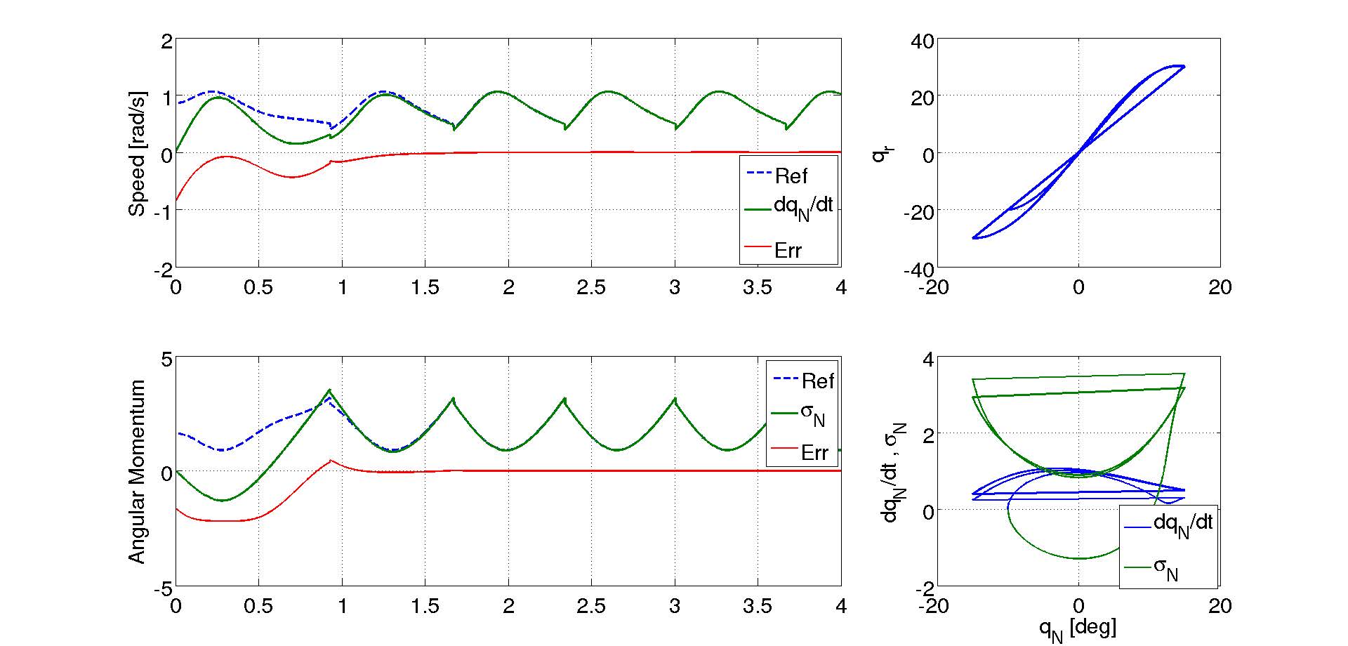
Figure 2: Complete control with exact model and starting outside $\mathcal{W}$ manifold.

Figure 3 show the results when some parametric errors are included on the model. Anyway, the control remains stable and can drive the robot close to the reference.

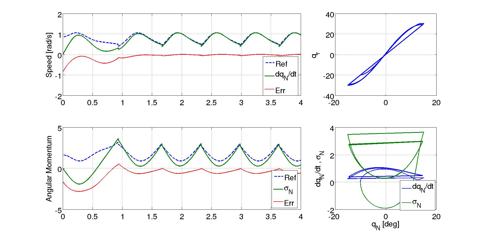
Figure 3: Complete control, model with parametric errors and starting outside $\mathcal{W}$ manifold.

6 Conclusions

We have derived a control law for the presented class of bipedal robots, so that the robot configuration will be tied to the absolute orientation. Also the speed of this absolute orientation and the angular momentum will follow predetermined references. As result, the robot will asymptotically converge to a walking gait at the same time as the average disc speed can be driven to zero (or any other desired value) by an appropriate offset in the reference for the angular momentum.

The stability of the proposed control was proved around some neighborhood of the nominal step and could be verified in numerical simulations. The simulations shows that the domain of attraction is somewhat big as the nominal step is reached even if the robot starts with no speed and the results could also be validated for some parametric errors

References

• Isidori (1995) Alberto Isidori. Nonlinear Control Systems. Springer-Verlag New York, Inc., Secaucus, NJ, USA, 3rd edition, 1995. ISBN 3540199160.
• Kieffer and Bale (1993) Jon Kieffer and Ramesh Bale. Walking Viability and Gait Synthesis for a Novel Class of Dynamically-Simple Bipeds. Informatica (Slovenia), 17(2), 1993.
• Peres (2008) Cauê Peres. Projeto de Robôs Bípedes com Dinâmica Simplifcada Modelagem, Controle e Síntese de Trajetórias. PhD thesis, Escola Politécnica da Universidade de São Paulo - USP, May 2008.
• Rouchon and Sira-Ramirez (2003) P. Rouchon and H. Sira-Ramirez. Control of the walking toy: a flatness approach. In American Control Conference, 2003. Proceedings of the 2003, volume 3, page 2018, 2003. 10.1109/ACC.2003.1243371.
• Spong and Vidyasagar (1989) M. W. Spong and M. Vidyasagar. Robot Dynamics and Control. John Wiley & Sons, 1989.
• Spong et al. (2000) Mark W. Spong, Rogelio Losano, and Robert Mahony. An almost Linear Biped. In Proceedings on the 39th IEEE Conference on Decision and Control, 2000.
• Westervelt et al. (2007) Eric R. Westervelt, Jessy W. Grizzle, Christine Chevallereau, Jun H. Choi, and Benjamin Morris. Feedback Control of Dynamic Bipedal Robot Locomotion. Taylor & Francis LLC, first edition, 2007.