Optimal preconditioning for the symmetric and non-symmetric coupling of adaptive finite elements and boundary elements

Abstract.

We analyze a multilevel diagonal additive Schwarz preconditioner for the adaptive coupling of FEM and BEM for a linear 2D Laplace transmission problem. We rigorously prove that the condition number of the preconditioned system stays uniformly bounded, independently of the refinement level and the local mesh-size of the underlying adaptively refined triangulations. Although the focus is on the non-symmetric Johnson-Nédélec one-equation coupling, the principle ideas also apply to other formulations like the symmetric FEM-BEM coupling. Numerical experiments underline our theoretical findings.

1. Introduction

There exist plenty of works on preconditioning of FEM-BEM coupling equations, covering mainly the symmetric coupling with quasi-uniform meshes, see [CKL98, FS09, HPPS03, HMS99, HS98, KS02, MS98] and the references therein. In contrast to that, only little is known on preconditioning of the non-symmetric Johnson-Nédélec coupling, see e.g. [Med98], and also on preconditioning of adaptive FEM-BEM couplings. It is the main goal of this paper to close this gap and to extend the existing analysis to the case of the (adaptive) symmetric as well as non-symmetric Johnson-Nédélec coupling [JN80]. For the symmetric coupling [Cos88, Han90], the approach of Bramble & Pasciak [BP88] applies, which guarantees positive definiteness and symmetry of the Galerkin matrix with respect to a special inner product [CKL98, HPPS03, KS02]. Therefore, efficient iterative solvers designed for symmetric and positive definite matrices are applicable. However, due to the non-symmetry, such an approach may not work for the Johnson-Nédélec coupling in general. In [Med98], it was assumed that the coupling boundary is smooth. Hence, the double-layer integral operator $\mathcal{K}$ is compact. The system matrix can therefore be split into a symmetric part plus a compact perturbation part $\mathbf{K}$ (the Galerkin matrix of the double-layer integral operator). Preconditioning is done only on the symmetric part with the theory of [BP88], and convergence results for iterative solvers can then be obtained by compact perturbation theory assuming that the mesh-size of the coarsest mesh is sufficiently small. In general, however, the coupling boundary is not smooth. Therefore, the preconditioner theory must not rely on compactness of $\mathcal{K}$.

To state the contributions of the current work, we consider the non-symmetric stiffness matrix of the (stabilized) Johnson-Nédélec coupling, which reads in block-form

(1) $$\mathbf{A}_{\mathcal{L}}:=\begin{pmatrix}\mathbf{A}_{A}&-\mathbf{M}^{T}\\ \tfrac{1}{2}\mathbf{M}-\mathbf{K}&\mathbf{A}_{\mathcal{V}}\end{pmatrix}+\mathbf{S}\mathbf{S}^{T}\in{\mathbb{R}}^{(N+M)\times(N+M)},$$

see Section 2 below. Here, $\mathbf{S}\in{\mathbb{R}}^{N+M}$ denotes an appropriate stabilization vector, which ensures positive definiteness of $\mathbf{A}_{\mathcal{L}}$. The $N\times N$ matrix block $\mathbf{A}_{A}$ is the (positive semi-definite) Galerkin matrix of the FEM part, and the $M\times M$ matrix block $\mathbf{A}_{\mathcal{V}}$ is the Galerkin matrix of the simple-layer integral operator $\mathcal{V}$. As in [FS09, MS98], we deal with block-diagonal preconditioners of the form

(2) $${\mathbf{P}}_{\mathcal{L}}=\begin{pmatrix}{\mathbf{P}}_{\mathcal{A}}&\boldsymbol{0}\\ \boldsymbol{0}&{\mathbf{P}}_{\mathcal{V}}\end{pmatrix}.$$

Here, the appropriate operator $\mathcal{A}:H^{1}(\Omega)\to(H^{1}(\Omega))^{*}$ induces a coercive, symmetric, and bounded bilinear form $\langle\mathcal{A}(\cdot)\,,\,(\cdot)\rangle\simeq\|\cdot\|_{H^{1}(\Omega)}^{2}$. The symmetric and positive definite matrices ${\mathbf{P}}_{\mathcal{A}}$ resp. ${\mathbf{P}}_{\mathcal{V}}$ are spectrally equivalent to the symmetric and positive definite Galerkin matrices $\mathbf{A}_{\mathcal{A}}$ resp. $\mathbf{A}_{\mathcal{V}}$, i.e.

(3a) $$d_{\mathcal{A}}\langle{\mathbf{P}}_{\mathcal{A}}\boldsymbol{X}\,,\,\boldsymbol{X}\rangle_{2} \leq\langle\mathbf{A}_{\mathcal{A}}\boldsymbol{X}\,,\,\boldsymbol{X}\rangle_{2}\leq D_{\mathcal{A}}\langle{\mathbf{P}}_{\mathcal{A}}\boldsymbol{X}\,,\,\boldsymbol{X}\rangle_{2}\quad\text{for all }\boldsymbol{X}\in{\mathbb{R}}^{N},$$

(3b) $$d_{\mathcal{V}}\langle{\mathbf{P}}_{\mathcal{V}}\boldsymbol{\Phi}\,,\,\boldsymbol{\Phi}\rangle_{2} \leq\langle\mathbf{A}_{\mathcal{V}}\boldsymbol{\Phi}\,,\,\boldsymbol{\Phi}\rangle_{2}\leq D_{\mathcal{V}}\langle{\mathbf{P}}_{\mathcal{V}}\boldsymbol{\Phi}\,,\,\boldsymbol{\Phi}\rangle_{2}\quad\text{for all }\boldsymbol{\Phi}\in{\mathbb{R}}^{M},$$

where $\mathbf{A}_{\mathcal{A}}$ is strongly related to the FEM block $\mathbf{A}_{A}$ of the FEM-BEM system (1), see (23)–(25) below. Inspired by [MS98], we prove that the condition number of ${\mathbf{P}}_{\mathcal{L}}^{-1}\mathbf{A}_{\mathcal{L}}$ as well as the number of iterations to reduce the relative residual by a factor $\tau$ in the preconditioned GMRES algorithm with inner product $\langle\cdot\,,\,\cdot\rangle_{{\mathbf{P}}_{\mathcal{L}}}$ depends only on $\max\{D_{\mathcal{A}},D_{\mathcal{V}}\}/\min\{d_{\mathcal{A}},d_{\mathcal{V}}\}$.

Usually, the condition number of Galerkin matrices $\mathbf{A}_{\mathcal{A}}$ and $\mathbf{A}_{\mathcal{V}}$ on adaptively refined meshes hinges on the global mesh-ratio as well as on the number of degrees of freedom. Therefore, the construction of optimal preconditioners for iterative solvers is a necessary task. Here, optimality is understood in the sense that the condition number of the preconditioned matrix is independent of the mesh-size and the degrees of freedom.

Very recently, it was proven in [XCH10] for 2D FEM with energy space $H^{1}$ that a local multilevel additive Schwarz preconditioner ${\mathbf{P}}_{\mathcal{A}}$ is optimal, i.e. the constants $d_{\mathcal{A}},D_{\mathcal{A}}$ in (3) are independent of the mesh-size, the number of degrees of freedom, and the number of levels. Here, “local” means, that scaling at each level is done only on newly created nodes plus neighbouring nodes, where the associated basis functions have changed. An analogous result for 2D and 3D hypersingular integral equations with energy space $H^{1/2}$ has been derived by the authors [FFPS13]. In [FFPS13, XCH10], the proofs rely on a stable space decomposition of the discrete subspaces in $H^{1}$ resp. $H^{1/2}$. Alternatively, [XCN09] provides stable subspace decompositions in $H^{1}$ for higher order elements in any dimension on bisection grids.

In the present work, we prove the optimality of some local multilevel additive Schwarz preconditioner ${\mathbf{P}}_{\mathcal{V}}$ for 2D weakly-singular integral equations with energy space $H^{-1/2}$. The proof is derived by postprocessing of the corresponding result for the hypersingular integral equation [FFPS13]. Combining this with the result of [XCH10], we prove optimality of ${\mathbf{P}}_{\mathcal{L}}$ for the FEM-BEM coupling.

Notation. Throughout the work, we explicitly state all constants and their dependencies in all statements of results. In proofs, however, we use the notation $a\lesssim b$ to abbreviate $a\leq Cb$ with a constant $C>0$ which is clear from the context. Moreover, $a\simeq b$ abbreviates $a\lesssim b\lesssim a$. Furthermore, the entries of a vector $\mathbf{b}$ or a matrix $\mathbf{A}$ are denoted by $(\mathbf{b})_{j}$ resp. $(\mathbf{A})_{jk}$. By $\langle\cdot\,,\,\cdot\rangle$, we denote the duality brackets between a Hilbert space ${\mathcal{H}}$ and its dual ${\mathcal{H}}^{*}$.

Outline. The remainder of this work is organized as follows: In Section 2, we recall the basic facts on the Johnson-Nédélec coupling and define the admissible mesh-refinement strategies. We also formulate the preconditioned GMRES Algorithm 3, which is required to state the main result (Theorem 4). In Section 3, we prove the spectral estimates (3). Section 4 adapts the analysis for the symmetric coupling [MS98] and contains the proof of the main result (Theorem 4). The short Section 5 deals with extensions of the developed theory to the symmetric coupling and the one-equation Bielak-MacCamy coupling. Numerical examples from Section 6 underline our theoretical predictions and conclude the work.

2. Johnson-Nédélec coupling and main result

2.1. Model problem and analytical setting

Let $\Omega\subset{\mathbb{R}}^{2}$ be a polygonal and simply connected domain with boundary $\Gamma=\partial\Omega$. We consider the following Laplace transmission problem in free space:

(4a) $$-{\rm div}(A\nabla u) =f \text{in }\Omega,$$

(4b) $$-\Delta u^{\rm ext} =0 \text{in }\Omega^{\rm ext}:={\mathbb{R}}^{2}\backslash\overline{\Omega},$$

(4c) $$u-u^{\rm ext} =u_{0} \text{on }\Gamma,$$

(4d) $$(A\nabla u-\nabla u^{\rm ext})\cdot\boldsymbol{n} =\phi_{0} \text{on }\Gamma,$$

(4e) $$|u^{\rm ext}(x)| ={\mathcal{O}}(1/|x|) \text{as }|x|\to\infty.$$

Here, $\boldsymbol{n}$ denotes the outer normal on $\Gamma$, and $A\in L^{\infty}(\Omega)$ satisfies $A(x)\in{\mathbb{R}}_{\rm sym}^{2\times 2}$ with uniform bounds on the maximal resp. minimal eigenvalue

(5) $$0<c_{A}:={\rm ess}\inf_{x\in\Omega}\lambda_{\rm min}(A(x))\leq{\rm ess}\sup_{x\in\Omega}\lambda_{\rm max}(A(x))=:C_{A}<\infty.$$

With $H^{1}(\Omega)$ resp. $H^{1/2}(\Gamma)$ and its dual $H^{-1/2}(\Gamma)=H^{1/2}(\Gamma)^{*}$, we denote the usual Sobolev spaces on $\Omega$ resp. $\Gamma$. For given data $f\in L^{2}(\Omega)$, $u_{0}\in H^{1/2}(\Gamma)$, and $\phi_{0}\in H^{-1/2}(\Gamma)$, it is well-known that the model problem (4) admits a unique solution $u\in H^{1}(\Omega)$, $u^{\rm ext}\in H_{\rm loc}^{1}(\Omega^{\rm ext})$ with finite energy $\nabla u^{\rm ext}\in L^{2}(\Omega^{\rm ext})$, if we impose the compatibility condition

(6) $$\langle f\,,\,1\rangle_{\Omega}+\langle\phi_{0}\,,\,1\rangle_{\Gamma}=0$$

to ensure the radiation condition (4e). Here, $\langle\cdot\,,\,\cdot\rangle_{\Omega}$ stands for the $L^{2}(\Omega)$ inner product, whereas $\langle\cdot\,,\,\cdot\rangle_{\Gamma}$ denotes the extended $L^{2}(\Gamma)$ inner product.

2.2. Johnson-Nédélec coupling

For the formulation of the Johnson-Nédélec coupling [JN80], the exterior solution (4b) is formulated by Green’s third formula. The latter gives rise to the simple-layer and double-layer integral operator

(7a) $$\mathcal{V}\in L(H^{-1/2+s}(\Gamma);H^{1/2+s}(\Gamma)),\quad \mathcal{V}\phi(x):=\int_{\Gamma}\,G(x,y)\phi(y)\,dy,$$

(7b) $$\mathcal{K}\in L(H^{1/2+s}(\Gamma);H^{1/2+s}(\Gamma)),\quad \mathcal{K}v(x):=\int_{\Gamma}\partial_{\boldsymbol{n}(y)}G(x,y)\,v(y)\,dy,$$

where $$G(x,y):=-\frac{1}{2\pi}\,\log|x-y| \partial_{\boldsymbol{n}}(\cdot) -1/2\leq s\leq 1/2$$ denotes the fundamental solution of the 2D Laplacian and is the normal derivative. Note that boundedness holds for all . In addition, our analysis requires the hypersingular integral operator

(7c) $$\mathcal{W}\in L(H^{1/2+s}(\Gamma);H^{-1/2+s}(\Gamma)),\quad \mathcal{W}v(x):=-\partial_{\boldsymbol{n}(x)}\int_{\Gamma}\partial_{\boldsymbol{n}(y)}G(x,y)\,v(y)\,dy,$$

where the integral is understood as finite part integral. It is known that $\mathcal{V}$ and $\mathcal{W}$ are symmetric in the sense of

(8) $$\langle\phi\,,\,\mathcal{V}\psi\rangle_{\Gamma}=\langle\psi\,,\,\mathcal{V}\phi\rangle_{\Gamma}\quad\text{and}\quad\langle\mathcal{W}v\,,\,w\rangle_{\Gamma}=\langle\mathcal{W}w\,,\,v\rangle_{\Gamma}$$

for all $\phi,\psi\in H^{-1/2}(\Gamma)$ and $v,w\in H^{1/2}(\Gamma)$. Moreover, the assumption ${\rm diam}(\Omega)<1$ ensures $H^{-1/2}(\Gamma)$-ellipticity of $\mathcal{V}$,

(9) $$c_{\mathcal{V}}\,\|\psi\|_{H^{-1/2}(\Gamma)}^{2}\leq\langle\psi\,,\,\mathcal{V}\psi\rangle_{\Gamma}\quad\text{for all }\psi\in H^{-1/2}(\Gamma).$$

Finally, $\mathcal{W}$ is semi-elliptic with kernel being the constant functions,

(10) $$\mathcal{W}1=0\quad\text{and}\quad c_{\mathcal{W}}\,\|v\|_{H^{1/2}(\Gamma)}^{2}\leq\langle\mathcal{W}v\,,\,v\rangle_{\Gamma}\quad\text{for all }v\in H^{1/2}(\Gamma)\text{ with }\int_{\Gamma}v\,dx=0.$$

The constants $c_{\mathcal{V}},c_{\mathcal{W}}>0$ depend only on $\Omega$.

With the definitions (7) of the layer integral operators, the model problem (4) is equivalently recast by the Johnson-Nédélec coupling: Given $f\in L^{2}(\Omega)$, $u_{0}\in H^{1/2}(\Gamma)$, and $\phi_{0}\in H^{-1/2}(\Gamma)$, find $(u,\phi)\in{\mathcal{H}}:=H^{1}(\Omega)\times H^{-1/2}(\Gamma)$ such that

(11a) $$\langle A\nabla u\,,\,\nabla v\rangle_{\Omega}-\langle\phi\,,\,v\rangle_{\Gamma} =\langle f\,,\,v\rangle_{\Omega}+\langle\phi_{0}\,,\,v\rangle_{\Gamma},$$

(11b) $$\langle\psi\,,\,(\tfrac{1}{2}-\mathcal{K})u+\mathcal{V}\phi\rangle_{\Gamma} =\langle\psi\,,\,(\tfrac{1}{2}-\mathcal{K})u_{0}\rangle_{\Gamma}$$

for all $(v,\psi)\in{\mathcal{H}}$. Setting $(u,\phi)=(1,0)=(v,\psi)$ in (11), we see that the (non-stabilized) linear operator associated to the left-hand side of (11) is indefinite. However, let $1/2\leq c_{\mathcal{K}}<1$ denote the contraction constant of the double-layer potential [SW01]. Following the analysis in [OS13, Say09, Ste11], also (stabilized) Galerkin formulations of (11) admit unique solutions, if the ellipticity constant $c_{A}$ from (5) satisfies

(12) $$c_{A}\geq c_{\mathcal{K}}/4$$

and if the equation is either explicitly stabilized [OS13, Ste11] or if the discrete subspace of $H^{-1/2}(\Gamma)$ contains the constant functions [Say09]. In [AFF⁺13a], the result of [Say09] is reproduced with a new proof. Introducing the notion of implicit stabilization, an equivalent elliptic operator equation of (11) is derived which fits in the frame of the Lax-Milgram lemma and thus leads to non-symmetric, but positive definite Galerkin matrices. The main result of [AFF⁺13a] reads as follows (and also holds for a strongly monotone, but nonlinear material tensor $A$):

Lemma 1.

Let (12) be satisfied. For $(u,\phi),(v,\psi)\in{\mathcal{H}}={\mathcal{X}}\times{\mathcal{Y}}$, define

(13a) $$\begin{split}\langle\mathcal{L}(u,\phi)\,,\,(v,\psi)\rangle&:=\langle A\nabla u\,,\,\nabla v\rangle_{\Omega}-\langle\phi\,,\,v\rangle_{\Gamma}+\langle\psi\,,\,(\tfrac{1}{2}-\mathcal{K})u+\mathcal{V}\phi\rangle_{\Gamma}\\ &\qquad+\langle 1\,,\,(\tfrac{1}{2}-\mathcal{K})u+\mathcal{V}\phi\rangle_{\Gamma}\langle 1\,,\,(\tfrac{1}{2}-\mathcal{K})v+\mathcal{V}\psi\rangle_{\Gamma}\end{split}$$

as well as

(13b) $$\begin{split}\langle F\,,\,(v,\psi)\rangle&:=\langle f\,,\,v\rangle_{\Omega}+\langle\phi_{0}\,,\,v\rangle_{\Gamma}+\langle\psi\,,\,(\tfrac{1}{2}-\mathcal{K})u_{0}\rangle_{\Gamma}\\ &\qquad+\langle 1\,,\,(\tfrac{1}{2}-\mathcal{K})u_{0}\rangle_{\Gamma}\langle 1\,,\,(\tfrac{1}{2}-\mathcal{K})v+\mathcal{V}\psi\rangle_{\Gamma}.\end{split}$$

Let ${\mathcal{X}}^{\ell}\subseteq{\mathcal{X}}$ and ${\mathcal{Y}}^{\ell}\subseteq{\mathcal{Y}}$ be arbitrary closed subspaces with $1\in{\mathcal{Y}}^{\ell}$. Then, the pair $(u_{\ell},\phi_{\ell})\in{\mathcal{H}}^{\ell}:={\mathcal{X}}^{\ell}\times{\mathcal{Y}}^{\ell}$ solves the Galerkin formulation of the Johnson-Nédélec coupling (11)

(14a) $$\langle A\nabla u_{\ell}\,,\,\nabla v_{\ell}\rangle_{\Omega}-\langle\phi_{\ell}\,,\,v_{\ell}\rangle_{\Gamma} =\langle f\,,\,v_{\ell}\rangle_{\Omega}+\langle\phi_{0}\,,\,v_{\ell}\rangle_{\Gamma},$$

(14b) $$\langle\psi_{\ell}\,,\,(\tfrac{1}{2}-\mathcal{K})u_{\ell}+\mathcal{V}\phi_{\ell}\rangle_{\Gamma} =\langle\psi_{\ell}\,,\,(\tfrac{1}{2}-\mathcal{K})u_{0}\rangle_{\Gamma}$$

for all $(v_{\ell},\psi_{\ell})\in{\mathcal{H}}^{\ell}$, if and only if it solves the operator formulation

(15) $$\begin{split}\langle\mathcal{L}(u_{\ell},\phi_{\ell})\,,\,(v_{\ell},\psi_{\ell})\rangle&=\langle F\,,\,(v_{\ell},\psi_{\ell})\rangle\end{split}$$

for all $(v_{\ell},\psi_{\ell})\in{\mathcal{H}}^{\ell}$. The operator $\mathcal{L}:{\mathcal{H}}\to{\mathcal{H}}^{*}$ is non-symmetric, but linear, continuous, and elliptic, and the constants

(16) $$c_{\mathcal{L}}:=\inf_{\boldsymbol{0}\neq(u,\phi)\in{\mathcal{H}}}\frac{\langle\mathcal{L}(u,\phi)\,,\,(u,\phi)\rangle}{\|(u,\phi)\|_{{\mathcal{H}}}^{2}}\quad\text{and}\quad C_{\mathcal{L}}:=\sup_{\boldsymbol{0}\neq(u,\phi)\in{\mathcal{H}}}\frac{\|\mathcal{L}(u,\phi)\|_{{\mathcal{H}}^{*}}}{\|(u,\phi)\|_{{\mathcal{H}}}}$$

satisfy $0<c_{\mathcal{L}}\leq C_{\mathcal{L}}<\infty$ and depend only on $c_{A}$ and $C_{A}$ from (5) as well as on $\Omega$. Moreover, $F\in{\mathcal{H}}^{*}$ is a continuous linear functional on ${\mathcal{H}}$. In particular, (15) (and hence also (14)) admits a unique solution $(u_{\ell},\phi_{\ell})\in{\mathcal{H}}^{\ell}$, and there holds the Céa-type estimate

(17) $$\|(u,\phi)-(u_{\ell},\phi_{\ell})\|_{{\mathcal{H}}}\leq\frac{C_{\mathcal{L}}}{c_{\mathcal{L}}}\inf\limits_{(v_{\ell},\psi_{\ell})\in{\mathcal{H}}^{\ell}}\|(u,\phi)-(v_{\ell},\psi_{\ell})\|_{{\mathcal{H}}},$$

where $(u,\phi)\in{\mathcal{H}}$ denotes the unique solution of the Johnson-Nédélec coupling (11).∎

2.3. Adaptive mesh-refinement and discrete spaces

\psfrag{T0}{}\psfrag{T1}{}\psfrag{T2}{}\psfrag{T3}{}\psfrag{T4}{}\psfrag{T12}{}\psfrag{T34}{}\includegraphics[width=99.58464pt]{nvb/bisec1_00}

\psfrag{T0}{}\psfrag{T1}{}\psfrag{T2}{}\psfrag{T3}{}\psfrag{T4}{}\psfrag{T12}{}\psfrag{T34}{}\includegraphics[width=99.58464pt]{nvb/bisec2left_00}

\psfrag{T0}{}\psfrag{T1}{}\psfrag{T2}{}\psfrag{T3}{}\psfrag{T4}{}\psfrag{T12}{}\psfrag{T34}{}\includegraphics[width=99.58464pt]{nvb/bisec2right_00}

\psfrag{T0}{}\psfrag{T1}{}\psfrag{T2}{}\psfrag{T3}{}\psfrag{T4}{}\psfrag{T12}{}\psfrag{T34}{}\includegraphics[width=99.58464pt]{nvb/bisec3_00}

\psfrag{T0}{}\psfrag{T1}{}\psfrag{T2}{}\psfrag{T3}{}\psfrag{T4}{}\psfrag{T12}{}\psfrag{T34}{}\includegraphics[width=99.58464pt]{nvb/bisec1_01}

\psfrag{T0}{}\psfrag{T1}{}\psfrag{T2}{}\psfrag{T3}{}\psfrag{T4}{}\psfrag{T12}{}\psfrag{T34}{}\includegraphics[width=99.58464pt]{nvb/bisec2left_01}

\psfrag{T0}{}\psfrag{T1}{}\psfrag{T2}{}\psfrag{T3}{}\psfrag{T4}{}\psfrag{T12}{}\psfrag{T34}{}\includegraphics[width=99.58464pt]{nvb/bisec2right_01}

\psfrag{T0}{}\psfrag{T1}{}\psfrag{T2}{}\psfrag{T3}{}\psfrag{T4}{}\psfrag{T12}{}\psfrag{T34}{}\includegraphics[width=99.58464pt]{nvb/bisec3_01}

Figure 1. For each triangle $T\in{\mathcal{T}}_{\ell}^{\Omega}$, there is one fixed reference edge, indicated by the double line (left, top). Refinement of $T$ is done by bisecting the reference edge, where its midpoint becomes a new node. The reference edges of the son triangles are opposite to this newest vertex (left, bottom). To avoid hanging nodes, one proceeds as follows: We assume that certain edges of $T$, but at least the reference edge, are marked for refinement (top). Using iterated newest vertex bisection, the element is then split into 2, 3, or 4 son triangles (bottom).

Let ${\mathcal{T}}_{0}^{\Omega}$ be a given conforming initial triangulation of $\Omega$ into compact and non-degenerate triangles. We suppose that a sequence ${\mathcal{T}}_{\ell+1}^{\Omega}={\rm refine}({\mathcal{T}}_{\ell}^{\Omega},\mathcal{M}_{\ell}^{\Omega})$ of refined triangulations is obtained by newest vertex bisection, see Figure 1, where ${\mathcal{T}}_{\ell+1}^{\Omega}$ is the coarsest conforming mesh such that all marked elements $T\in\mathcal{M}_{\ell}^{\Omega}\subseteq{\mathcal{T}}_{\ell}^{\Omega}$ have been bisected. For our analysis, the set $\emptyset\neq\mathcal{M}_{\ell}^{\Omega}\subseteq{\mathcal{T}}_{\ell}^{\Omega}$ of marked elements is arbitrary, but in practice obtained from local a posteriori refinement indicators, see e.g. [AFF⁺13a]. We note that newest vertex bisection guarantees uniform shape regularity in the sense that

(18) $$\sup\limits_{T\in{\mathcal{T}}_{\ell}^{\Omega}}\frac{{\rm diam}(T)}{|T|^{1/2}}\leq\gamma<\infty\quad\text{for all }\ell\in{\mathbb{N}}_{0},$$

where $\gamma$ depends only on the initial mesh ${\mathcal{T}}_{0}^{\Omega}$, see e.g. [Ver13, KPP13] and the references therein.

Let ${\mathcal{T}}_{0}^{\Gamma}$ be a given initial partition of the coupling boundary $\Gamma$ into compact line segments. We suppose that a sequence ${\mathcal{T}}_{\ell+1}^{\Gamma}={\rm refine}({\mathcal{T}}_{\ell}^{\Gamma},\mathcal{M}_{\ell}^{\Gamma})$ of refined partitions is obtained by bisection, where the refined elements $T\in{\mathcal{T}}_{\ell}^{\Gamma}\backslash{\mathcal{T}}_{\ell+1}^{\Gamma}$ are refined into two sons $T^{\prime},T^{\prime\prime}\in{\mathcal{T}}_{\ell+1}^{\Gamma}\backslash{\mathcal{T}}_{\ell}^{\Gamma}$ of half length, i.e. $T=T^{\prime}\cup T^{\prime\prime}$ with ${\rm diam}(T^{\prime})={\rm diam}(T^{\prime\prime})={\rm diam}(T)/2$ and where at least the marked elements $T\in\mathcal{M}_{\ell}^{\Gamma}\subseteq{\mathcal{T}}_{\ell}^{\Gamma}$ are refined, i.e. $\mathcal{M}_{\ell}^{\Gamma}\subseteq{\mathcal{T}}_{\ell}^{\Gamma}\backslash{\mathcal{T}}_{\ell+1}^{\Gamma}$. In addition, we suppose that the meshes are uniformly $\gamma$-shape regular in the sense that

(19) $$\frac{{\rm diam}(T)}{{\rm diam}(T^{\prime})}\leq\gamma<\infty\quad\text{for all }T,T^{\prime}\in{\mathcal{T}}_{\ell}^{\Gamma}\text{ with }T\cap T^{\prime}\neq\emptyset\text{ and all }\ell\in{\mathbb{N}}_{0},$$

where $\gamma$ depends only on the initial partition ${\mathcal{T}}_{0}^{\Gamma}$. Possible choices include the 1D bisection algorithms from [AFF⁺13b]. A further choice is to consider the partition ${\mathcal{T}}_{\ell}^{\Gamma}:={\mathcal{T}}_{\ell}^{\Omega}|_{\Gamma}$ of $\Gamma$ which is induced by the triangulation ${\mathcal{T}}_{\ell}^{\Omega}$ of $\Omega$. Formally, such a coupling of ${\mathcal{T}}_{\ell}^{\Omega}$ and ${\mathcal{T}}_{\ell}^{\Gamma}$ is not required for the analysis, but simplifies the implementation and is therefore used in the numerical experiments of Section 6.

In this work, we consider lowest-order Galerkin elements. We approximate functions $u\in H^{1}(\Omega)$ by functions $u_{\ell}\in{\mathcal{X}}^{\ell}$ and functions $\phi\in H^{-1/2}(\Gamma)$ by functions $\phi_{\ell}\in{\mathcal{Y}}^{\ell}$, where

(20) $${\mathcal{X}}^{\ell} :=\big{\{}v\in C(\Omega)\,:\,v|_{T}\text{ is affine for all }T\in{\mathcal{T}}_{\ell}^{\Omega}\big{\}},$$

(21) $${\mathcal{Y}}^{\ell} :=\big{\{}\psi\in L^{2}(\Gamma)\,:\,\psi|_{T}\text{ is constant for all }T\in{\mathcal{T}}_{\ell}^{\Gamma}\big{\}}.$$

Let ${\mathcal{N}}_{\ell}^{\Omega}$ denote the set of nodes of the triangulation ${\mathcal{T}}_{\ell}^{\Omega}$, and let ${\mathcal{N}}_{\ell}^{\Gamma}$ denote the set of nodes of the triangulation ${\mathcal{T}}_{\ell}^{\Gamma}$. For $z\in{\mathcal{N}}_{\ell}^{\Omega}$ resp. $z\in{\mathcal{N}}_{\ell}^{\Gamma}$, we define the patch $\omega_{\ell}^{\Omega}(z):=\big{\{}T\in{\mathcal{T}}_{\ell}^{\Omega}\,:\,z\in T\big{\}}$ resp. $\omega_{\ell}^{\Gamma}(z):=\big{\{}T\in{\mathcal{T}}_{\ell}^{\Gamma}\,:\,z\in T\big{\}}$. For the construction of optimal multilevel preconditioners on adaptively refined triangulations, we need the following subsets of ${\mathcal{N}}_{\ell}^{\Omega}$ resp. ${\mathcal{N}}_{\ell}^{\Gamma}$:

(22a) $$\widetilde{\mathcal{N}}_{0}^{\Omega} :={\mathcal{N}}_{0}^{\Omega}, \widetilde{\mathcal{N}}_{\ell}^{\Omega} :={\mathcal{N}}_{\ell}^{\Omega}\backslash{\mathcal{N}}_{\ell-1}^{\Omega}\cup\big{\{}z\in{\mathcal{N}}_{\ell-1}^{\Omega}\,:\,\omega_{\ell}^{\Omega}(z)\subsetneqq\omega_{\ell-1}^{\Omega}(z)\big{\}}\quad\text{for }\ell\geq 1,$$

(22b) $$\widetilde{\mathcal{N}}_{0}^{\Gamma} :={\mathcal{N}}_{0}^{\Gamma} \widetilde{\mathcal{N}}_{\ell}^{\Gamma} :={\mathcal{N}}_{\ell}^{\Gamma}\backslash{\mathcal{N}}_{\ell-1}^{\Gamma}\cup\big{\{}z\in{\mathcal{N}}_{\ell-1}^{\Gamma}\,:\,\omega_{\ell}^{\Gamma}(z)\subsetneqq\omega_{\ell-1}^{\Gamma}(z)\big{\}}\quad\text{for }\ell\geq 1.$$

The sets $\widetilde{\mathcal{N}}_{\ell}^{\Omega}$ resp. $\widetilde{\mathcal{N}}_{\ell}^{\Gamma}$ thus consist of the new nodes plus the old nodes, where the corresponding patches have changed. A visualization of $\widetilde{\mathcal{N}}_{\ell}^{\Omega}$ is given in Figure 2. For each node $z\in{\mathcal{N}}_{\ell}^{\Omega}$, $\eta_{z}^{\ell}\in{\mathcal{X}}^{\ell}$ denotes the associated hat-function with $\eta_{z}^{\ell}(z^{\prime})=\delta_{zz^{\prime}}$ for all $z^{\prime}\in{\mathcal{N}}_{\ell}^{\Omega}$, where $\delta_{zz^{\prime}}$ is Kronecker’s delta.

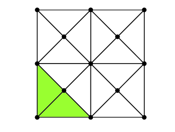
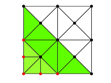
Figure 2. The left figure shows a FEM mesh ${\mathcal{T}}_{\ell-1}^{\Omega}$, where the two elements (green) are marked for refinement. Bisection of these two elements provides the mesh ${\mathcal{T}}_{\ell}^{\Omega}$ (right), where two new nodes are created. The set $\widetilde{\mathcal{N}}_{\ell}^{\Omega}$ consists of these new nodes plus their immediate neighbours (red), where the corresponding patches have changed. The union of the support of the basis functions associated to nodes in $\widetilde{\mathcal{N}}_{\ell}^{\Omega}$ is given by the light- and dark-green areas in the right figure.

2.4. Galerkin system and block-diagonal preconditioning

Let $\{\eta_{z_{j}}^{\ell}\}_{j=1}^{N_{\ell}}$ with $N_{\ell}:=\#{\mathcal{N}}_{\ell}^{\Omega}$ denote the nodal basis of ${\mathcal{X}}^{\ell}$, and let $\{\psi_{T_{j}}\}_{j=1}^{M_{\ell}}$ with $M_{\ell}:=\#{\mathcal{T}}_{\ell}^{\Gamma}$ denote a basis of ${\mathcal{Y}}^{\ell}$, where $\psi_{T_{j}}$ denotes the characteristic function on $T_{j}\in{\mathcal{T}}_{\ell}^{\Gamma}$. The Galerkin matrix $\mathbf{A}_{\mathcal{L}}=\mathbf{A}_{\mathcal{L}}^{\ell}\in{\mathbb{R}}^{(N_{\ell}+M_{\ell})\times(N_{\ell}+M_{\ell})}$ of the operator $\mathcal{L}$ has the form

$$\mathbf{A}_{\mathcal{L}}=\begin{pmatrix}\mathbf{A}_{A}&-\mathbf{M}^{T}\\ \tfrac{1}{2}\mathbf{M}-\mathbf{K}&\mathbf{A}_{\mathcal{V}}\end{pmatrix}+\mathbf{S}\mathbf{S}^{T},$$

where the block matrices $\mathbf{A}_{A}\in{\mathbb{R}}^{N_{\ell}\times N_{\ell}}$, $\mathbf{A}_{\mathcal{V}}\in{\mathbb{R}}^{M_{\ell}\times M_{\ell}}$, $\mathbf{M}\in{\mathbb{R}}^{M_{\ell}\times N_{\ell}}$, and $\mathbf{K}\in{\mathbb{R}}^{M_{\ell}\times N_{\ell}}$ as well as the stabilization (column) vector $\mathbf{S}\in{\mathbb{R}}^{N_{\ell}+M_{\ell}}$ are given by

(23a) $$(\mathbf{A}_{A})_{jk} =\langle A\nabla\eta_{z_{k}}^{\ell}\,,\,\nabla\eta_{z_{j}}^{\ell}\rangle_{\Omega}\quad\text{for }j,k=1,\dots,N_{\ell},$$

(23b) $$(\mathbf{A}_{\mathcal{V}})_{jk} =\langle\psi_{T_{j}}\,,\,\mathcal{V}\psi_{T_{k}}\rangle_{\Gamma}\quad\text{for }j,k=1,\dots,M_{\ell},$$

(23c) $$(\mathbf{M})_{jk} =\langle\psi_{T_{j}}\,,\,(\eta_{z_{k}}^{\ell})|_{\Gamma}\rangle_{\Gamma}\quad\text{for }j=1,\dots,M_{\ell},k=1,\dots,N_{\ell},$$

(23d) $$(\mathbf{K})_{jk} =\langle\psi_{T_{j}}\,,\,\mathcal{K}(\eta_{z_{k}}^{\ell})|_{\Gamma}\rangle_{\Gamma}\quad\text{for }j=1,\dots,M_{\ell},k=1,\dots,N_{\ell},$$

(23e) $$\begin{split}(\mathbf{S})_{j}&=\langle 1\,,\,(\tfrac{1}{2}-\mathcal{K})(\eta_{z_{j}}^{\ell})|_{\Gamma}\rangle_{\Gamma}\quad\text{for }j=1,\dots,N_{\ell},\\ (\mathbf{S})_{j+N_{\ell}}&=\langle 1\,,\,\mathcal{V}\psi_{T_{j}}\rangle_{\Gamma}\quad\text{for }j=1,\dots,M_{\ell}.\end{split}$$

We stress that $\mathbf{A}_{A}$ as well as $\mathbf{M}$ are sparse, whereas $\mathbf{A}_{\mathcal{V}}$ is dense. Note that the number of non-zeros in the matrix $\mathbf{K}$ is bounded by $\#({\mathcal{N}}_{\ell}^{\Omega}\cap\Gamma)\cdot M_{\ell}$. Moreover, the application of the rank-$1$ stabilization matrix $\mathbf{S}\mathbf{S}^{T}$ can be implemented efficiently with complexity ${\mathcal{O}}(N_{\ell}+M_{\ell})$ for use with an iterative solver.

The discrete variational formulation (15) is equivalent to solving the following linear system of equations: Find $\mathbf{U}\in{\mathbb{R}}^{N_{\ell}+M_{\ell}}$ such that

(24) $$\mathbf{A}_{\mathcal{L}}\mathbf{U}=\mathbf{F}\in{\mathbb{R}}^{N_{\ell}+M_{\ell}},$$

where the right-hand side vector $\mathbf{F}\in{\mathbb{R}}^{N_{\ell}+M_{\ell}}$ reads

$$(\mathbf{F})_{j} =\langle F\,,\,(\eta_{z_{j}}^{\ell},0)\rangle\quad\text{for }j=1,\dots,N_{\ell},$$

$$(\mathbf{F})_{j+N_{\ell}} =\langle F\,,\,(0,\psi_{T_{j}})\rangle\quad\text{for }j=1,\dots,M_{\ell}.$$

To formulate our block-diagonal preconditioner, we require an appropriate operator $\mathcal{A}$ which is related to the FEM-domain part of $\mathcal{L}$. The next lemma follows from a Rellich compactness argument, since $\mathcal{K}c=-c/2$ for all constants $c\in{\mathbb{R}}$. Details are analogous to, e.g., [AFF⁺13a, Lemma 10] and therefore left to the reader.

Lemma 2.

For $u,v\in H^{1}(\Omega)$, define

(25a) $$\langle\mathcal{A}u\,,\,v\rangle:=\langle A\nabla u\,,\,\nabla v\rangle_{\Omega}+\langle 1\,,\,(\tfrac{1}{2}-\mathcal{K})u\rangle_{\Gamma}\langle 1\,,\,(\tfrac{1}{2}-\mathcal{K})v\rangle_{\Gamma}.$$

Then, the operator $$\mathcal{A}:H^{1}(\Omega)\to(H^{1}(\Omega))^{*}$$ is linear, symmetric, continuous, and elliptic, and the constants

(25b) $$c_{\mathcal{A}}:=\inf_{0\neq u\in H^{1}(\Omega)}\frac{\langle\mathcal{A}u\,,\,u\rangle}{\|u\|_{H^{1}(\Omega)}^{2}}\quad\text{and}\quad C_{\mathcal{A}}:=\sup_{0\neq u\in H^{1}(\Omega)}\frac{\|\mathcal{A}u\|_{(H^{1}(\Omega))^{*}}}{\|u\|_{H^{1}(\Omega)}}$$

satisfy $0<c_{\mathcal{A}}\leq C_{\mathcal{A}}<\infty$ and depend only on $c_{A}$ and $C_{A}$ from (5) as well as on $\Omega$.∎

In this work, we investigate block-diagonal preconditioners of the form

(26) $${\mathbf{P}}_{\mathcal{L}}=\begin{pmatrix}{\mathbf{P}}_{\mathcal{A}}&\boldsymbol{0}\\ \boldsymbol{0}&{\mathbf{P}}_{\mathcal{V}}\end{pmatrix},$$

where ${\mathbf{P}}_{\mathcal{A}}$ is a “good” approximation of the Galerkin matrix $\mathbf{A}_{\mathcal{A}}$ corresponding to the operator $\mathcal{A}$ from Lemma 2 with respect to the nodal basis of ${\mathcal{X}}^{\ell}$, and ${\mathbf{P}}_{\mathcal{V}}$ is a “good” approximation of the Galerkin matrix $\mathbf{A}_{\mathcal{V}}$. Our construction below ensures that ${\mathbf{P}}_{\mathcal{A}},{\mathbf{P}}_{\mathcal{V}}$ and hence ${\mathbf{P}}$ are symmetric and positive definite.

Instead of (24), we solve the preconditioned system

(27) $${\mathbf{P}}_{\mathcal{L}}^{-1}\mathbf{A}_{\mathcal{L}}\mathbf{U}={\mathbf{P}}_{\mathcal{L}}^{-1}\mathbf{F}\in{\mathbb{R}}^{N_{\ell}+M_{\ell}}.$$

For this non-symmetric system of linear equations, we use a preconditioned GMRES algorithm [SS86], which will be discussed in the following subsection. The preconditioned Galerkin matrix reads in block form

(28) $${\mathbf{P}}_{\mathcal{L}}^{-1}\mathbf{A}_{\mathcal{L}}=\begin{pmatrix}{\mathbf{P}}_{\mathcal{A}}^{-1}&\boldsymbol{0}\\ \boldsymbol{0}&{\mathbf{P}}_{\mathcal{V}}^{-1}\end{pmatrix}\left[\begin{pmatrix}\mathbf{A}_{A}&-\mathbf{M}^{T}\\ \tfrac{1}{2}\mathbf{M}-\mathbf{K}&\mathbf{A}_{\mathcal{V}}\end{pmatrix}+\mathbf{S}\mathbf{S}^{T}\right].$$

2.5. Preconditioned GMRES algorithm

Let ${\mathbf{P}}\in{\mathbb{R}}^{N\times N}$ denote a symmetric and positive definite matrix and let $\mathbf{A}\in{\mathbb{R}}^{N\times N}$ denote a (possibly) non-symmetric, but positive definite matrix. Let, $\mathbf{E}^{k}\in{\mathbb{R}}^{N}$ denote the standard unit vector with entries $(\mathbf{E}^{k})_{j}=\delta_{kj}$. The preconditioned GMRES algorithm reads as follows.

Algorithm 3 (GMRES).

Input: Matrices ${\mathbf{P}},\mathbf{A}\in{\mathbb{R}}^{N\times N}$, right-hand side vector $\mathbf{F}\in{\mathbb{R}}^{N}$, initial guess $\mathbf{U}^{0}\in{\mathbb{R}}^{N}$, relative tolerance $\tau>0$, and maximum number of iterations $K\in{\mathbb{N}}$ with $K\leq N$.

• Allocate memory for the matrix $\mathbf{H}\in{\mathbb{R}}^{(K+1)\times K}$, the vectors $\mathbf{V}^{i}\in{\mathbb{R}}^{N}$, $i=1,\dots,K$, $\mathbf{W}\in{\mathbb{R}}^{N}$, $\mathbf{U}\in{\mathbb{R}}^{N}$, $\mathbf{R}^{0}\in{\mathbb{R}}^{N}$ and $\mathbf{R}\in{\mathbb{R}}^{N}$.

• Compute initial residual $\mathbf{R}^{0}\leftarrow{\mathbf{P}}^{-1}(\mathbf{F}-\mathbf{A}\mathbf{U}^{0})$ and $\mathbf{V}^{1}\leftarrow\mathbf{R}^{0}/\|\mathbf{R}^{0}\|_{{\mathbf{P}}}$.

• Set counter $k\leftarrow 1$, and initialize $(\mathbf{H})_{ij}\leftarrow 0$ for all $i=1,\dots,K+1,j=1,\dots,K$.

Iterate the following steps (i)–(vii):

• Compute $\mathbf{W}\leftarrow{\mathbf{P}}^{-1}\mathbf{A}\mathbf{V}^{k}$.

• For all $i=1,\dots,k$ compute

  $$(\mathbf{H})_{ik}\leftarrow\langle\mathbf{W}\,,\,\mathbf{V}^{i}\rangle_{\mathbf{P}}\quad\text{and}\quad\mathbf{W}\leftarrow\mathbf{W}-\mathbf{V}^{i}(\mathbf{H})_{ik}.$$

• Compute $(\mathbf{H})_{k+1,k}\leftarrow\|\mathbf{W}\|_{{\mathbf{P}}}$.

• Define the sub-matrix $\overline{\mathbf{H}}^{k}\in{\mathbb{R}}^{(k+1)\times k}$ with entries $(\overline{\mathbf{H}}^{k})_{ij}:=(\mathbf{H})_{ij}$ for $i=1,\dots,k+1,j=1,\dots,k$ and compute

  $$\mathbf{Y}^{k}\leftarrow\operatorname*{arg\,min}\limits_{\mathbf{Y}\in{\mathbb{R}}^{k}}\|\|\mathbf{R}_{0}\|_{{\mathbf{P}}}\mathbf{E}^{1}-\overline{\mathbf{H}}^{k}\mathbf{Y}\|_{2}.$$

• Compute $\mathbf{U}\leftarrow\mathbf{U}^{0}+(\mathbf{V}^{1}\cdots\mathbf{V}^{k})\mathbf{Y}^{k}$ and $\mathbf{R}\leftarrow{\mathbf{P}}^{-1}(\mathbf{F}-\mathbf{A}\mathbf{U})$.

• Stop iteration if $\|\mathbf{R}\|_{{\mathbf{P}}}\leq\tau\|\mathbf{R}^{0}\|_{{\mathbf{P}}}$ or $k\geq K$.

• Otherwise, compute $\mathbf{V}^{k+1}\leftarrow\mathbf{W}/(\mathbf{H})_{k+1,k}$, update counter $k\leftarrow k+1$, and goto (iv).

Output: $\mathbf{U}$, $k$, and $\|\mathbf{R}\|_{{\mathbf{P}}}/\|\mathbf{R}^{0}\|_{{\mathbf{P}}}$.

Note that for ${\mathbf{P}}$ being the identity matrix, Algorithm 3 is the usual GMRES algorithm with inner product $\langle\cdot\,,\,\cdot\rangle_{2}$, see e.g. [SS86]. The main memory consumption is given by the vectors $\mathbf{V}^{i}\in{\mathbb{R}}^{N}$, while the matrix $\overline{\mathbf{H}}^{k}\in{\mathbb{R}}^{(k+1)\times k}$ in step (iv) is a sub-block of the matrix $\mathbf{H}\in{\mathbb{R}}^{(K+1)\times K}$ and thus does not need to be stored explicitly.

As is often the case for multilevel preconditioners, the application of ${\mathbf{P}}^{-1}$ on a vector is known, whereas the application of ${\mathbf{P}}$ is unknown. We therefore note that the GMRES Algorithm 3 can be implemented without using ${\mathbf{P}}$ to compute the inner products $\langle\cdot\,,\,\cdot\rangle_{\mathbf{P}}$ and the norms $\|\cdot\|_{{\mathbf{P}}}$. To this end, one replaces the computation of $\mathbf{V}^{1}$ by $\widetilde{\mathbf{V}}^{1}\leftarrow(\mathbf{F}-\mathbf{A}\mathbf{U}^{0})/\|\mathbf{R}^{0}\|_{{\mathbf{P}}}$, where $\|\mathbf{R}^{0}\|_{{\mathbf{P}}}^{2}=\langle{\mathbf{P}}^{-1}(\mathbf{F}-\mathbf{A}\mathbf{U}^{0})\,,\,\mathbf{F}-\mathbf{A}\mathbf{U}^{0}\rangle_{2}$. Then, $\mathbf{V}^{1}\leftarrow{\mathbf{P}}^{-1}\widetilde{\mathbf{V}}^{1}$. In step (i), we compute $\widetilde{\mathbf{W}}\leftarrow\mathbf{A}\mathbf{V}^{k}$ instead of $\mathbf{W}$. Step (ii) is replaced by $(\mathbf{H})_{ik}\leftarrow\langle{\mathbf{P}}^{-1}\widetilde{\mathbf{W}}\,,\,\mathbf{V}^{i}\rangle_{\mathbf{P}}=\langle\widetilde{\mathbf{W}}\,,\,\mathbf{V}^{i}\rangle_{2}$ and $\widetilde{\mathbf{W}}\leftarrow\widetilde{\mathbf{W}}-\widetilde{\mathbf{V}}^{i}(\mathbf{H})_{ik}$. Instead of step (iii), we then compute $(\mathbf{H})_{k+1,k}\leftarrow\|{\mathbf{P}}^{-1}\widetilde{\mathbf{W}}\|_{{\mathbf{P}}}=\sqrt{\langle{\mathbf{P}}^{-1}\widetilde{\mathbf{W}}\,,\,\widetilde{\mathbf{W}}\rangle_{2}}$. Note that $\|\mathbf{R}\|_{{\mathbf{P}}}^{2}=\langle{\mathbf{P}}^{-1}(\mathbf{F}-\mathbf{A}\mathbf{U})\,,\,\mathbf{F}-\mathbf{A}\mathbf{U}\rangle_{2}$ in step (vi). Lastly, in step (vii) we replace the computation of $\mathbf{V}^{k+1}$ by $\widetilde{\mathbf{V}}^{k+1}\leftarrow\widetilde{\mathbf{W}}/(\mathbf{H})_{k+1,k}$ and $\mathbf{V}^{k+1}\leftarrow{\mathbf{P}}^{-1}\widetilde{\mathbf{V}}^{k+1}$.

2.6. Local multilevel preconditioner and main result

For both the FEM part ${\mathbf{P}}_{\mathcal{A}}$ and BEM part ${\mathbf{P}}_{\mathcal{V}}$ in (26), we will use local multilevel preconditioners which are optimal in the sense that the condition numbers of the preconditioned systems are independent of the number of levels $L$ and the mesh-size $h_{L}$.

For the preconditioner ${\mathbf{P}}_{\mathcal{A}}$, we use an additive Schwarz multilevel diagonal preconditioner similar to the one in [XCH10]. Recall $\widetilde{\mathcal{N}}_{\ell}^{\Omega}\subseteq{\mathcal{N}}_{\ell}^{\Omega}$ from (22) Define

(29) $$\widetilde{\mathcal{X}}^{\ell}:={\rm span}\big{\{}\eta_{z}^{\ell}\,:\,z\in\widetilde{\mathcal{N}}_{\ell}^{\Omega}\big{\}}\subseteq{\mathcal{X}}^{\ell}.$$

Let $\widetilde{\mathcal{I}}^{\ell}:\widetilde{\mathcal{X}}^{\ell}\to{\mathcal{X}}^{L}$ denote the canonical embedding with matrix representation $\widetilde{\mathbf{I}}^{\ell}\in{\mathbb{R}}^{\widetilde{N}_{\ell}^{\Omega}\times N_{L}^{\Omega}}$ and $\widetilde{N}_{\ell}^{\Omega}:=\#\widetilde{\mathcal{N}}_{\ell}^{\Omega}$. Furthermore, let $\widetilde{\mathbf{D}}_{\mathcal{A}}^{\ell}$ denote the diagonal of the Galerkin matrix $\widetilde{\mathbf{A}}_{\mathcal{A}}^{\ell}$ with respect to the local set of nodes $\widetilde{\mathcal{N}}_{\ell}^{\Omega}$, i.e. $(\widetilde{\mathbf{A}}_{\mathcal{A}}^{\ell})_{jk}=\langle\mathcal{A}\eta_{z_{k}}^{\ell}\,,\,\eta_{z_{j}}^{\ell}\rangle$ for $j,k=1,\dots,\widetilde{N}_{\ell}^{\Omega}$ and $(\widetilde{\mathbf{D}}_{\mathcal{A}}^{\ell})_{jk}:=\delta_{jk}(\widetilde{\mathbf{A}}_{\mathcal{A}}^{\ell})_{jj}$. Then, our local multilevel diagonal preconditioner ${\mathbf{P}}_{\mathcal{A}}$ is defined via

(30) $${\mathbf{P}}_{\mathcal{A}}^{-1}:=({\mathbf{P}}_{\mathcal{A}}^{L})^{-1}:=\sum_{\ell=0}^{L}\widetilde{\mathbf{I}}^{\ell}(\widetilde{\mathbf{D}}_{\mathcal{A}}^{\ell})^{-1}(\widetilde{\mathbf{I}}^{\ell})^{T}.$$

From the definition, we see that this preconditioner corresponds to a diagonal scaling on each level, where scaling is done on the local subset $\widetilde{\mathcal{N}}_{\ell}^{\Omega}$ only.

For all boundary nodes $z\in{\mathcal{N}}_{\ell}^{\Gamma}$, let

(31) $$\zeta_{z}^{\ell}\in{\mathcal{Z}}^{\ell}:=\big{\{}v\in C(\Gamma)\,:\,v|_{T}\text{ is affine for all }T\in{\mathcal{T}}_{\ell}^{\Gamma}\big{\}}$$

denote the boundary hat-function with $\zeta_{z}^{\ell}(z^{\prime})=\delta_{zz^{\prime}}$ for all $z^{\prime}\in{\mathcal{N}}_{\ell}^{\Gamma}$. To construct an efficient preconditioner ${\mathbf{P}}_{\mathcal{V}}$ for the weakly-singular integral operator $\mathcal{V}$ in 2D, we use the Haar-basis functions $\chi_{z}^{\ell}:=(\zeta_{z}^{\ell})^{\prime}$ for all $z\in{\mathcal{N}}_{\ell}^{\Gamma}$. Recall $\widetilde{\mathcal{N}}_{\ell}^{\Gamma}\subseteq{\mathcal{N}}_{\ell}^{\Gamma}$ from (22). Let $\widetilde{N}_{\ell}^{\Gamma}:=\#\widetilde{\mathcal{N}}_{\ell}^{\Gamma}$. Define the local subspaces

(32) $$\widetilde{\mathcal{Y}}^{\ell}:={\rm span}\big{\{}\chi_{z}^{\ell}\,:\,z\in\widetilde{\mathcal{N}}_{\ell}^{\Gamma}\big{\}}\subsetneqq{\mathcal{Y}}^{\ell},\qquad\widetilde{\mathcal{Z}}^{\ell}:={\rm span}\big{\{}\zeta_{z}^{\ell}\,:\,z\in\widetilde{\mathcal{N}}_{\ell}^{\Gamma}\big{\}}\subseteq{\mathcal{Z}}^{\ell},$$

and the matrix $\widetilde{\mathbf{H}}^{\ell}\in{\mathbb{R}}^{M_{\ell}\times\widetilde{N}_{\ell}^{\Gamma}}$ which represents the Haar-basis functions with respect to the canonical basis $\big{\{}\psi_{T}\,:\,\psi_{T}\text{ is characteristic function on }T\in{\mathcal{T}}_{\ell}^{\Gamma}\big{\}}$ of ${\mathcal{Y}}^{\ell}$, i.e.

$$\chi_{z_{k}}^{\ell}=\sum_{j=1}^{M_{\ell}}(\widetilde{\mathbf{H}}^{\ell})_{jk}\psi_{T_{j}}\quad\text{for }j=1,\dots,M_{\ell},\quad k=1,\dots,\widetilde{N}_{\ell}^{\Gamma}.$$

Maue’s formula [Mau49] states the relation

(33) $$\langle\mathcal{W}v\,,\,w\rangle_{\Gamma}=\langle\mathcal{V}v^{\prime}\,,\,w^{\prime}\rangle_{\Gamma}\quad\text{for all }v,w\in H^{1}(\Gamma)$$

and thus reveals the identity

$$\Big{(}(\widetilde{\mathbf{H}}^{\ell})^{T}\mathbf{A}_{\mathcal{V}}^{\ell}\widetilde{\mathbf{H}}^{\ell}\Big{)}_{jk}=\langle\mathcal{V}\chi_{z_{k}}^{\ell}\,,\,\chi_{z_{j}}^{\ell}\rangle_{\Gamma}=\langle\mathcal{W}\zeta_{z_{k}}^{\ell}\,,\,\zeta_{z_{j}}^{\ell}\rangle_{\Gamma}=:(\widetilde{\mathbf{A}}_{\mathcal{W}}^{\ell})_{jk}\quad\text{for }j,k=1,\dots,\widetilde{N}_{\ell}^{\Gamma}$$

for the Galerkin matrix $\widetilde{\mathbf{A}}_{\mathcal{W}}^{\ell}$ of the hypersingular integral operator with respect to the nodes $\widetilde{\mathcal{N}}_{\ell}^{\Gamma}$. Let $\widetilde{\mathbf{D}}_{\mathcal{W}}^{\ell}$ denote the diagonal of $\widetilde{\mathbf{A}}_{\mathcal{W}}^{\ell}$, and let $\mathcal{J}^{\ell}:{\mathcal{Y}}^{\ell}\to{\mathcal{Y}}^{L}$ denote the canonical embedding with matrix representation $\mathbf{J}^{\ell}$. Moreover, define $D:=\langle 1\,,\,\mathcal{V}1\rangle_{\Gamma}$ and let $\mathbf{1}\in{\mathbb{R}}^{M_{L}}$ denote the vector with constant entries $(\mathbf{1})_{j}=1$ for all $j=1,\dots M_{L}$. Then, our multilevel diagonal preconditioner ${\mathbf{P}}_{\mathcal{V}}$ for the weakly-singular integral operator reads

(34) $${\mathbf{P}}_{\mathcal{V}}^{-1}:=({\mathbf{P}}_{\mathcal{V}}^{L})^{-1}:=\mathbf{1}D^{-1}\mathbf{1}^{T}+\sum_{\ell=0}^{L}\mathbf{J}^{\ell}\widetilde{\mathbf{H}}^{\ell}(\widetilde{\mathbf{D}}_{\mathcal{W}}^{\ell})^{-1}(\widetilde{\mathbf{H}}^{\ell})^{T}(\mathbf{J}^{\ell})^{T}.$$

The following theorem is the main result of this work. Let ${\rm cond}_{\mathbf{C}}(\mathbf{A})=\|\mathbf{A}\|_{\mathbf{C}}\|\mathbf{A}^{-1}\|_{\mathbf{C}}$ denote the condition number of the matrix $\mathbf{A}$ with respect to the norm $\|\cdot\|_{\mathbf{C}}$ induced by the symmetric and positive definite matrix $\mathbf{C}$.

Theorem 4.

Let ${\mathbf{P}}_{\mathcal{A}}$ resp. ${\mathbf{P}}_{\mathcal{V}}$ denote the multilevel preconditioners defined in (30) resp. (34). Then, the condition number

(35) $${\rm cond}_{{\mathbf{P}}_{\mathcal{L}}}({\mathbf{P}}_{\mathcal{L}}^{-1}\mathbf{A}_{\mathcal{L}})\leq C<\infty$$

is uniformly bounded. Moreover, the $j$-th residual $\mathbf{R}^{j}$ from the preconditioned GMRES Algorithm 3 with ${\mathbf{P}}={\mathbf{P}}_{\mathcal{L}}$ from (26) satisfies

(36) $$\|\mathbf{R}^{j}\|_{{\mathbf{P}}_{\mathcal{L}}}\leq q_{\rm GMRES}^{j}\|\mathbf{R}^{0}\|_{{\mathbf{P}}_{\mathcal{L}}}.$$

The constants $C>0$ and $0<q_{\rm GMRES}<1$ depend only on $\Omega$, the ellipticity and continuity constants of the material tensor $A$ from (5), the initial triangulations ${\mathcal{T}}_{0}^{\Omega}$ and ${\mathcal{T}}_{0}^{\Gamma}$, as well as on the mesh-refinement strategy chosen.

3. Spectral estimates for $\mathbf{A}_{\mathcal{A}}$ and $\mathbf{A}_{\mathcal{V}}$

In this section, we provide spectral estimates for the matrices $\mathbf{A}_{\mathcal{A}}$, $\mathbf{A}_{\mathcal{V}}$. In particular, the equivalences $\langle\mathbf{A}_{\mathcal{A}}\boldsymbol{X}\,,\,\boldsymbol{X}\rangle_{2}\simeq\langle{\mathbf{P}}_{\mathcal{A}}\boldsymbol{X}\,,\,\boldsymbol{X}\rangle_{2}$ for $\boldsymbol{X}\in{\mathbb{R}}^{N_{L}}$ as well as $\langle\mathbf{A}_{\mathcal{V}}\boldsymbol{\Phi}\,,\,\boldsymbol{\Phi}\rangle_{2}\simeq\langle{\mathbf{P}}_{\mathcal{V}}\boldsymbol{\Phi}\,,\,\boldsymbol{\Phi}\rangle_{2}$ for $\boldsymbol{\Phi}\in{\mathbb{R}}^{M_{L}}$ are optimal in the sense, that the involved constants are independent of $L$ and $h_{L}$.

The remainder of this section is organized as follows: In Section 3.1, we focus on the optimality of the preconditioner ${\mathbf{P}}_{\mathcal{A}}$, which follows from [WC06, XCH10]. In Section 3.2, we analyze the preconditioner ${\mathbf{P}}_{\mathcal{V}}$ and prove optimality thereof. Note that optimality of ${\mathbf{P}}_{\mathcal{V}}$ for uniform meshes has already been proved in [TS96], where $\widetilde{\mathcal{N}}_{\ell}^{\Omega}={\mathcal{N}}_{\ell}^{\Omega}$ and $\widetilde{\mathcal{N}}_{\ell}^{\Gamma}={\mathcal{N}}_{\ell}^{\Gamma}$, while optimality on adaptive meshes is a particular contribution of the present work.

3.1. Optimality of the multilevel preconditioner ${\mathbf{P}}_{\mathcal{A}}$

Define the local projection operators ${\mathfrak{A}}_{z}^{\ell}:{\mathcal{X}}^{L}\to{\mathcal{X}}_{z}^{\ell}:={\rm span}\{\eta_{z}^{\ell}\}$ by

(37) $$\langle{\mathfrak{A}}_{z}^{\ell}v\,,\,w_{z}^{\ell}\rangle_{\mathcal{A}}=\langle v\,,\,w_{z}^{\ell}\rangle_{\mathcal{A}}\quad\text{for all }w_{z}^{\ell}\in{\mathcal{X}}_{z}^{\ell},$$

and the multilevel additive Schwarz preconditioner

(38) $${\mathfrak{A}}_{\rm AS}:=\sum_{\ell=0}^{L}\sum_{z\in\widetilde{\mathcal{N}}_{\ell}}{\mathfrak{A}}_{z}^{\ell}\,:\,{\mathcal{X}}^{L}\to{\mathcal{X}}^{L}.$$

A straightforward calculation shows the identity

(39) $$\langle{\mathbf{P}}_{\mathcal{A}}^{-1}\mathbf{A}_{\mathcal{A}}\boldsymbol{X}\,,\,\boldsymbol{X}\rangle_{\mathbf{A}_{\mathcal{A}}}=\langle{\mathfrak{A}}_{\rm AS}v\,,\,v\rangle_{\mathcal{A}},$$

where $v\in{\mathcal{H}}^{L}$ is given by $v=\sum_{j=1}^{N_{L}}(\boldsymbol{X})_{j}\eta_{z_{j}}^{L}$, and $N_{L}:=\#{\mathcal{N}}_{L}^{\Omega}$ denotes the number of nodes in the FEM domain. Thus, bounds for the extremal eigenvalues of the operator ${\mathfrak{A}}_{\rm AS}$ provide bounds for the extremal eigenvalues of the preconditioned system.

Theorem 5.

The preconditioner matrix ${\mathbf{P}}_{\mathcal{A}}$ is symmetric and positive definite. There holds

(40) $$d_{\mathcal{A}}\langle{\mathbf{P}}_{\mathcal{A}}\boldsymbol{X}\,,\,\boldsymbol{X}\rangle_{2}\leq\langle\mathbf{A}_{\mathcal{A}}\boldsymbol{X}\,,\,\boldsymbol{X}\rangle_{2}\leq D_{\mathcal{A}}\langle{\mathbf{P}}_{\mathcal{A}}\boldsymbol{X}\,,\,\boldsymbol{X}\rangle_{2}\quad\text{for all }\boldsymbol{X}\in{\mathbb{R}}^{N_{L}}.$$

The constants $d_{\mathcal{A}},D_{\mathcal{A}}$ depend only on $\Omega$, the initial triangulation ${\mathcal{T}}_{0}^{\Omega}$, as well as the use of newest vertex bisection for mesh-refinement.

Proof.

There holds a similar result to [XCH10, Theorem 4.2] for the additive Schwarz operator ${\mathfrak{A}}_{\rm AS}$, i.e., ${\mathfrak{A}}_{\rm AS}$ is $\langle\cdot\,,\,\cdot\rangle_{\mathcal{A}}$-symmetric and there holds for all $v\in{\mathcal{X}}^{L}$

(41) $$\langle{\mathfrak{A}}_{\rm AS}v\,,\,v\rangle_{\mathcal{A}}\simeq\langle\mathcal{A}v\,,\,v\rangle$$

where the hidden constants depend only on $\Omega$, the initial triangulation ${\mathcal{T}}_{0}^{\Omega}$, as well as on the mesh-refinement chosen. In particular, the proof of the equivalence (41) follows the lines of [XCH10, Section 4.1]. The two key ingredients of the proof are the results [WC06, Lemma 3.2–3.3], which also hold for the problem considered in this work. ∎

3.2. Optimality of the multilevel preconditioner ${\mathbf{P}}_{\mathcal{V}}$

In this section we prove that the optimal additive Schwarz preconditioner for the hypersingular integral operator provided in [FFPS13], which is based on a space decomposition of lowest-order hat-functions, induces optimality of the additive Schwarz operator for the weakly-singular integral operator. The key ingredient of the proof is Maue’s formula (33), which allows us, roughly speaking, to change between the $H^{1/2}$ and $H^{-1/2}$ norms. For uniform meshes, a similar approach, which uses a generalised antiderivative operator [HS96], is considered in [TS96]. The remainder of this section can be seen as an alternate proof of the results from [TS96, Section 3] as well as an extension to locally refined meshes.

Theorem 6.

The preconditioner matrix ${\mathbf{P}}_{\mathcal{V}}$ is symmetric and positive definite. There holds

(42) $$d_{\mathcal{V}}\langle{\mathbf{P}}_{\mathcal{V}}\boldsymbol{\Phi}\,,\,\boldsymbol{\Phi}\rangle_{2}\leq\langle\mathbf{A}_{\mathcal{V}}\boldsymbol{\Phi}\,,\,\boldsymbol{\Phi}\rangle_{2}\leq D_{\mathcal{V}}\langle{\mathbf{P}}_{\mathcal{V}}\boldsymbol{\Phi}\,,\,\boldsymbol{\Phi}\rangle_{2}\quad\text{for all }\boldsymbol{\Phi}\in{\mathbb{R}}^{M_{L}}.$$

The constants $d_{\mathcal{V}},D_{\mathcal{V}}$ depend only on $\Gamma$, the initial triangulation ${\mathcal{T}}_{0}^{\Gamma}$, and the chosen mesh-refinement. Moreover, the eigenvalues of the preconditioned matrix ${\mathbf{P}}_{\mathcal{V}}^{-1}\mathbf{A}_{\mathcal{V}}$ are bounded by

(43) $$d_{\mathcal{V}}\leq\lambda_{\rm min}({\mathbf{P}}_{\mathcal{V}}^{-1}\mathbf{A}_{\mathcal{V}})\leq\lambda_{\rm max}({\mathbf{P}}_{\mathcal{V}}^{-1}\mathbf{A}_{\mathcal{V}})\leq D_{\mathcal{V}}.$$

According to (7a), and (8)–(9), $\langle\phi\,,\,\psi\rangle_{\mathcal{V}}:=\langle\mathcal{V}\phi\,,\,\psi\rangle_{\Gamma}$ defines a scalar product with equivalent norm $\|\phi\|_{\mathcal{V}}^{2}:=\langle\phi\,,\,\phi\rangle_{\mathcal{V}}$ on $H^{-1/2}(\Gamma)$. According to (7c), (8), (10), and the Rellich compactness theorem, $\langle u\,,\,v\rangle_{\mathcal{W}}:=\langle\mathcal{W}u\,,\,v\rangle_{\Gamma}+\langle u\,,\,1\rangle_{\Gamma}\langle v\,,\,1\rangle_{\Gamma}$ defines a scalar product with equivalent norm $\|u\|_{\mathcal{W}}^{2}:=\langle u\,,\,u\rangle_{\mathcal{W}}$ on $H^{1/2}(\Gamma)$.

We need to define a subspace decomposition of the space ${\mathcal{Y}}^{L}$. To that end, we make use of the Haar basis functions $\chi_{z}^{\ell}=(\zeta_{z}^{\ell})^{\prime}$, which are the arclength derivatives of the hat functions $\zeta_{z}^{\ell}$. Then, ${\mathcal{Z}}^{L}={\rm span}\big{\{}\zeta_{z}^{L}\,:\,z\in{\mathcal{N}}^{L}\big{\}}$ can be decomposed into

$${\mathcal{Z}}^{L}=\sum_{\ell=0}^{L}\sum_{z\in\widetilde{\mathcal{N}}_{\ell}^{\Gamma}}{\mathcal{Z}}_{z}^{\ell}\quad\text{with }{\mathcal{Z}}_{z}^{\ell}:={\rm span}\{\zeta_{z}^{\ell}\}.$$

Moreover, simple calculations with $\langle\chi_{z}^{\ell}\,,\,1\rangle_{\Gamma}=0$ show that

$${\mathcal{Y}}^{L}={\mathcal{Y}}^{00}\oplus\sum_{\ell=0}^{L}\sum_{z\in\widetilde{\mathcal{N}}_{\ell}^{\Gamma}}{\mathcal{Y}}_{z}^{\ell}\quad\text{with }{\mathcal{Y}}^{00}:={\rm span}\{1\}\text{ and }{\mathcal{Y}}_{z}^{\ell}:={\rm span}\{\chi_{z}^{\ell}\}$$

defines a (direct sum) decomposition of ${\mathcal{Y}}^{L}$ into ${\mathcal{Y}}^{00}$ and an additive Schwarz space. With this, we define the additive Schwarz operator

(44) $$\mathfrak{V}_{\rm AS}={\mathfrak{V}}^{00}+\sum_{\ell=0}^{L}\sum_{z\in\widetilde{\mathcal{N}}_{\ell}^{\Gamma}}{\mathfrak{V}}_{z}^{\ell},$$

where ${\mathfrak{V}}^{00}$ resp. ${\mathfrak{V}}_{z}^{\ell}$ are defined for all $\phi\in{\mathcal{Y}}^{L}$ via

(45a) $$\langle{\mathfrak{V}}^{00}\phi\,,\,\phi_{0}\rangle_{\mathcal{V}} =\langle\phi\,,\,\phi_{0}\rangle_{\mathcal{V}}\quad\text{for all }\phi_{0}\in{\mathcal{Y}}^{00}\quad\text{resp.}$$

(45b) $$\langle{\mathfrak{V}}_{z}^{\ell}\phi\,,\,\phi_{z}^{\ell}\rangle_{\mathcal{V}} =\langle\phi\,,\,\phi_{z}^{\ell}\rangle_{\mathcal{V}}\quad\text{for all }\phi_{z}^{\ell}\in{\mathcal{Y}}_{z}^{\ell}.$$

We note that the symmetry of the orthogonal projectors ${\mathfrak{V}}^{00}$ resp. ${\mathfrak{V}}_{z}^{\ell}$ implies that also $\mathfrak{V}_{\rm AS}$ is symmetric

(46) $$\langle\mathfrak{V}_{\rm AS}\phi\,,\,\psi\rangle_{\mathcal{V}}=\langle\phi\,,\,\mathfrak{V}_{\rm AS}\phi\rangle_{\mathcal{V}}\quad\text{for all }\phi,\psi\in{\mathcal{Y}}^{L}.$$

Our analysis of $\mathfrak{V}_{\rm AS}$ builds on own results [FFPS13] on the additive Schwarz operator associated to the hypersingular integral equation,

(47) $$\mathfrak{W}_{\rm AS}=\sum_{\ell=0}^{L}\sum_{z\in\widetilde{\mathcal{N}}_{\ell}^{\Gamma}}{\mathfrak{W}}_{z}^{\ell},\quad\text{where }\langle{\mathfrak{W}}_{z}^{\ell}v\,,\,v_{z}^{\ell}\rangle_{\mathcal{W}}=\langle v\,,\,v_{z}^{\ell}\rangle_{\mathcal{W}}\quad\text{for all }v_{z}^{\ell}\in{\mathcal{X}}_{z}^{\ell}.$$

The analysis of [FFPS13] provides the following result.

Lemma 7 ([FFPS13, Proposition 4 ]).

The operator $\mathfrak{W}_{\rm AS}:{\mathcal{Z}}^{L}\to{\mathcal{Z}}^{L}$ is symmetric and satisfies

$$C_{\ref{consthyp:lb}}\|v\|_{\mathcal{W}}^{2}\leq\langle\mathfrak{W}_{\rm AS}v\,,\,v\rangle_{\mathcal{W}}\leq C_{\ref{consthyp:ub}}\|v\|_{\mathcal{W}}^{2}\quad\text{for all }v\in{\mathcal{Z}}^{L},$$

where the constants $C_{\ref{consthyp:lb}},C_{\ref{consthyp:ub}}>0$ depend only on $\Gamma$, the initial triangulation ${\mathcal{T}}_{0}^{\Gamma}$, as well as on the chosen mesh-refinement. ∎

For each $\phi\in{\mathcal{Y}}^{L}$, we follow [TS96] and split

(48) $$\phi=\phi_{0}+\widetilde{\phi}\quad\text{with unique }\phi_{0}=\langle\phi\,,\,1\rangle_{\Gamma}/|\Gamma|\in{\mathcal{Y}}^{00}\,\text{and }\widetilde{\phi}\in\sum_{\ell=0}^{L}\sum_{z\in\widetilde{\mathcal{N}}_{\ell}^{\Gamma}}{\mathcal{Y}}_{z}^{\ell}.$$

Let us introduce a mechanism to switch between the $H^{1/2}$ and $H^{-1/2}$ norms. For $\widetilde{\phi}\in{\mathcal{Y}}_{*}^{L}:=\{\phi\in{\mathcal{Y}}^{L}\,:\,\langle\phi\,,\,1\rangle_{\Gamma}=0\}$, there exists a unique function $\widetilde{v}\in{\mathcal{Z}}_{*}^{L}:=\{v\in{\mathcal{Z}}^{L}\,:\,\langle v\,,\,1\rangle_{\Gamma}=0\}$ such that

(49) $$\widetilde{\phi}=(\widetilde{v})^{\prime}.$$

To see this, let $\widetilde{\phi}\in{\mathcal{Y}}_{*}^{L}$ with

(50) $$\widetilde{\phi}=\sum_{\ell=0}^{L}\sum_{z\in\widetilde{\mathcal{N}}_{\ell}^{\Gamma}}\alpha_{z}^{\ell}\chi_{z}^{\ell}\quad\text{and define}\quad v:=\sum_{\ell=0}^{L}\sum_{z\in\widetilde{\mathcal{N}}_{\ell}^{\Gamma}}\alpha_{z}^{\ell}\zeta_{z}^{\ell}\in{\mathcal{Z}}^{L}.$$

Then, $\widetilde{v}:=v-\langle v\,,\,1\rangle_{\Gamma}/|\Gamma|\in{\mathcal{Z}}_{*}^{L}$, and it holds $(\widetilde{v})^{\prime}=v^{\prime}=\widetilde{\phi}$ as $\chi_{z}^{\ell}=(\zeta_{z}^{\ell})^{\prime}$. Maue’s formula (33) provides the important identities

(51) $$\langle\mathcal{W}\zeta_{z}^{\ell}\,,\,\zeta_{z}^{\ell}\rangle_{\Gamma}=\langle\mathcal{V}\chi_{z}^{\ell}\,,\,\chi_{z}^{\ell}\rangle_{\Gamma}\quad\text{as well as}\quad\langle\mathcal{W}\widetilde{v}\,,\,\widetilde{v}\rangle_{\Gamma}=\langle\mathcal{V}\widetilde{\phi}\,,\,\widetilde{\phi}\rangle_{\Gamma}.$$

We stress that (51) allows to switch between the spaces $H^{1/2}$ and $H^{-1/2}$. This is the heart of the proof of the following proposition.

Proposition 8.

The operator $\mathfrak{V}_{\rm AS}:{\mathcal{Y}}^{L}\to{\mathcal{Y}}^{L}$ is symmetric (46), and it holds

(52) $$C_{\ref{constslp_lb}}\|\psi\|_{\mathcal{V}}^{2}\leq\langle\mathfrak{V}_{\rm AS}\psi\,,\,\psi\rangle_{\mathcal{V}}\leq C_{\ref{constslp_ub}}\|\psi\|_{\mathcal{V}}^{2}\quad\text{for all }\psi\in{\mathcal{Y}}^{L}.$$

The constants $C_{\ref{constslp_lb}},C_{\ref{constslp_ub}}>0$ depend only on $\Gamma$, the initial triangulation ${\mathcal{T}}_{0}^{\Gamma}$, as well as on the bisection algorithm from Section 2.3.

For the proof of Proposition 8 we need the following result, see e.g. [Zha92], where the first part is known as Lions’ lemma.

Lemma 9.

(i)  Let $c>0$ and $\psi\in{\mathcal{Y}}^{L}$. Suppose that there exists a decomposition $\psi=\psi_{0}+\sum_{\ell=0}^{L}\sum_{z\in\widetilde{\mathcal{N}}_{\ell}^{\Gamma}}\psi_{z}^{\ell}$ with $\psi_{0}\in{\mathcal{Y}}^{00},\psi_{z}^{\ell}\in{\mathcal{Y}}_{z}^{\ell}$ such that

(53) $$\|\psi_{0}\|_{\mathcal{V}}^{2}+\sum_{\ell=0}^{L}\sum_{z\in\widetilde{\mathcal{N}}_{\ell}^{\Gamma}}\|\psi_{z}^{\ell}\|_{\mathcal{V}}^{2}\leq c^{-1}\|\psi\|_{\mathcal{V}}^{2}.$$

Then it follows, $c\|\psi\|_{\mathcal{V}}^{2}\leq\langle\mathfrak{V}_{\rm AS}\psi\,,\,\psi\rangle_{\mathcal{V}}$.

(ii)  Let $C>0$ and $\psi\in{\mathcal{Y}}^{L}$. Suppose that for all decompositions $\psi=\psi_{0}+\sum_{\ell=0}^{L}\sum_{z\in\widetilde{\mathcal{N}}_{\ell}^{\Gamma}}\psi_{z}^{\ell}$ with $\psi_{0}\in{\mathcal{Y}}^{00}$ and $\psi_{z}^{\ell}\in{\mathcal{Y}}_{z}^{\ell}$ holds

(54) $$\|\psi\|_{\mathcal{V}}^{2}\leq C\big{(}\|\psi_{0}\|_{\mathcal{V}}^{2}+\sum_{\ell=0}^{L}\sum_{z\in\widetilde{\mathcal{N}}_{\ell}^{\Gamma}}\|\psi_{z}^{\ell}\|_{\mathcal{V}}^{2}\big{)}.$$

Then, it follows $\langle\mathfrak{V}_{\rm AS}\psi\,,\,\psi\rangle_{\mathcal{V}}\leq C\|\psi\|_{\mathcal{V}}^{2}$.

Proof of Proposition 8, lower bound in (52).

By means of Lemma 9, we have to provide a stable subspace decomposition. For $\phi\in{\mathcal{Y}}^{L}$, we consider the unique decomposition $\phi=\phi_{0}+\widetilde{\phi}$ from (48). With $\phi_{0}=\langle\phi\,,\,1\rangle_{\Gamma}/|\Gamma|$, we infer

(55) $$\|\phi_{0}\|_{\mathcal{V}}=\frac{\langle\phi\,,\,1\rangle_{\Gamma}}{|\Gamma|}\|1\|_{\mathcal{V}}\leq\frac{\|\phi\|_{H^{-1/2}(\Gamma)}\|1\|_{H^{1/2}(\Gamma)}}{|\Gamma|}\|1\|_{\mathcal{V}}\lesssim\|\phi\|_{\mathcal{V}}.$$

Moreover, there exists $\widetilde{v}\in{\mathcal{Z}}_{*}^{L}$, such that $(\widetilde{v})^{\prime}=\widetilde{\phi}$. The abstract result [Zha92, Lemma 3.1] states

(56) $$\lambda_{\rm min}(\mathfrak{W}_{\rm AS})=\min\limits_{v\in{\mathcal{Z}}^{L}}\frac{\|v\|_{\mathcal{W}}^{2}}{\min\limits_{\sum_{\ell=0}^{L}\sum_{z\in\widetilde{\mathcal{N}}_{\ell}^{\Gamma}}v_{z}^{\ell}=v}\sum_{\ell=0}^{L}\sum_{z\in\widetilde{\mathcal{N}}_{\ell}^{\Gamma}}\|v_{z}^{\ell}\|_{\mathcal{W}}^{2}},$$

since $\mathfrak{W}_{\rm AS}$ is a finite sum of symmetric projectors. Lemma 7 provides uniform boundedness of the Rayleigh quotient $\langle\mathfrak{W}_{\rm AS}v\,,\,v\rangle_{\mathcal{W}}/\|v\|_{\mathcal{W}}^{2}\geq C_{\ref{consthyp:lb}}>0$. Thus, $\lambda_{\rm min}(\mathfrak{W}_{\rm AS})\geq C_{\ref{consthyp:lb}}>0$ is uniformly bounded, and we infer from (56) the existence of a decomposition $\widetilde{v}=\sum_{\ell=0}^{L}\sum_{z\in\widetilde{\mathcal{N}}_{\ell}^{\Gamma}}v_{z}^{\ell}$ with $v_{z}^{\ell}\in{\mathcal{Z}}_{z}^{\ell}$ such that

(57) $$\sum_{\ell=0}^{L}\sum_{z\in\widetilde{\mathcal{N}}_{\ell}^{\Gamma}}\|v_{z}^{\ell}\|_{\mathcal{W}}^{2}\lesssim\|\widetilde{v}\|_{\mathcal{W}}^{2}.$$

This provides a decomposition of $\widetilde{\phi}$ into functions $\phi_{z}^{\ell}=(v_{z}^{\ell})^{\prime}\in{\mathcal{Y}}_{z}^{\ell}$ by

(58) $$\widetilde{\phi}=(\widetilde{v})^{\prime}=:\sum_{\ell=0}^{L}\sum_{z\in\widetilde{\mathcal{N}}_{\ell}^{\Gamma}}\phi_{z}^{\ell}.$$

The identities from (51) imply

(59) $$\sum_{\ell=0}^{L}\sum_{z\in\widetilde{\mathcal{N}}_{\ell}^{\Gamma}}\|\phi_{z}^{\ell}\|_{\mathcal{V}}^{2}=\sum_{\ell=0}^{L}\sum_{z\in\widetilde{\mathcal{N}}_{\ell}^{\Gamma}}\langle\mathcal{V}\phi_{z}^{\ell}\,,\,\phi_{z}^{\ell}\rangle_{\Gamma}=\sum_{\ell=0}^{L}\sum_{z\in\widetilde{\mathcal{N}}_{\ell}^{\Gamma}}\langle\mathcal{W}v_{z}^{\ell}\,,\,v_{z}^{\ell}\rangle_{\Gamma}$$

The estimate $\langle\mathcal{W}v_{z}^{\ell}\,,\,v_{z}^{\ell}\rangle_{\Gamma}\leq\|v_{z}^{\ell}\|_{\mathcal{W}}^{2}$ and (57) prove

(60) $$\sum_{\ell=0}^{L}\sum_{z\in\widetilde{\mathcal{N}}_{\ell}^{\Gamma}}\langle\mathcal{W}v_{z}^{\ell}\,,\,v_{z}^{\ell}\rangle_{\Gamma}\leq\sum_{\ell=0}^{L}\sum_{z\in\widetilde{\mathcal{N}}_{\ell}^{\Gamma}}\|v_{z}^{\ell}\|_{\mathcal{W}}^{2}\lesssim\|\widetilde{v}\|_{\mathcal{W}}^{2}.$$

Since $\langle\widetilde{v}\,,\,1\rangle_{\Gamma}=0$, there holds $\|\widetilde{v}\|_{\mathcal{W}}^{2}=\langle\mathcal{W}\widetilde{v}\,,\,\widetilde{v}\rangle_{\Gamma}$. This, (59)–(60), and Maue’s formula (51) yield

(61) $$\sum_{\ell=0}^{L}\sum_{z\in\widetilde{\mathcal{N}}_{\ell}^{\Gamma}}\|\phi_{z}^{\ell}\|_{\mathcal{V}}^{2}\lesssim\langle\mathcal{W}\widetilde{v}\,,\,\widetilde{v}\rangle_{\Gamma}=\langle\mathcal{V}\widetilde{\phi}\,,\,\widetilde{\phi}\rangle_{\Gamma}=\|\widetilde{\phi}\|_{\mathcal{V}}^{2}.$$

Recall that $\widetilde{\phi}=\phi-\phi_{0}$. With (55), the triangle inequality yields

(62) $$\|\phi_{0}\|_{\mathcal{V}}^{2}+\sum_{\ell=0}^{L}\sum_{z\in\widetilde{\mathcal{N}}_{\ell}^{\Gamma}}\|\phi_{z}^{\ell}\|_{\mathcal{V}}^{2}\lesssim\|\phi_{0}\|_{\mathcal{V}}^{2}+\|\widetilde{\phi}\|_{\mathcal{V}}^{2}\lesssim\|\phi_{0}\|_{\mathcal{V}}^{2}+\|\phi\|_{\mathcal{V}}^{2}\lesssim\|\phi\|_{\mathcal{V}}^{2},$$

where the hidden constants depend only on $\Gamma$, the initial triangulation ${\mathcal{T}}_{0}^{\Gamma}$, as well as the chosen mesh-refinement strategy. By means of Lemma 9 (i), this proves the lower bound in (52). ∎

Proof of Proposition 8, upper bound in (52).

Recall the unique splitting $\phi=\phi_{0}+\widetilde{\phi}$ from (48). Let $\sum_{\ell=0}^{L}\sum_{z\in\widetilde{\mathcal{N}}_{\ell}^{\Gamma}}\phi_{z}^{\ell}=\widetilde{\phi}$ denote an arbitrary splitting of $\widetilde{\phi}\in\sum_{\ell=0}^{L}\sum_{z\in\widetilde{\mathcal{N}}_{\ell}^{\Gamma}}{\mathcal{Y}}_{z}^{\ell}$. Note that $\phi_{z}^{\ell}=\alpha_{z}^{\ell}\chi_{z}^{\ell}$ for some $\alpha_{z}^{\ell}\in{\mathbb{R}}$. We define $\widetilde{v}$ as

(63) $$\widetilde{v}:=\sum_{\ell=0}\sum_{z\in\widetilde{\mathcal{N}}_{\ell}^{\Gamma}}v_{z}^{\ell}\quad\text{with }v_{z}^{\ell}:=\alpha_{z}^{\ell}\zeta_{z}^{\ell}$$

and stress that $\widetilde{\phi}=(\widetilde{v})^{\prime}$ as well as $\phi_{z}^{\ell}=(v_{z}^{\ell})^{\prime}$. The abstract result [Zha92, Lemma 3.1] states

(64) $$\lambda_{\rm max}(\mathfrak{W}_{\rm AS})=\max_{v\in{\mathcal{Z}}^{L}}\frac{\|v\|_{\mathcal{W}}^{2}}{\min\limits_{\sum_{\ell=0}^{L}\sum_{z\in\widetilde{\mathcal{N}}_{\ell}^{\Gamma}}v_{z}^{\ell}=v}\sum_{\ell=0}^{L}\sum_{z\in\widetilde{\mathcal{N}}_{\ell}^{\Gamma}}\|v_{z}^{\ell}\|_{\mathcal{W}}^{2}},$$

since $\mathfrak{W}_{\rm AS}$ is a finite sum of symmetric projections. From Lemma 7, we get uniform boundedness of the Rayleigh quotient $\langle\mathfrak{W}_{\rm AS}v\,,\,v\rangle_{\mathcal{W}}/\|v\|_{\mathcal{W}}^{2}\leq C_{\ref{consthyp:ub}}$. Thus, $\lambda_{\rm max}(\mathfrak{W}_{\rm AS})\leq C_{\ref{consthyp:ub}}<\infty$ is uniformly bounded. Then, (64) yields

(65) $$\|\widetilde{v}\|_{\mathcal{W}}^{2}\lesssim\sum_{\ell=0}^{L}\sum_{z\in\widetilde{\mathcal{N}}_{\ell}^{\Gamma}}\|v_{z}^{\ell}\|_{\mathcal{W}}^{2}.$$

Together with Maue’s formula (51), the definition (63), and the norm equivalence

$$\|v_{z}^{\ell}\|_{\mathcal{W}}^{2}\simeq\|v_{z}^{\ell}\|_{H^{1/2}(\Gamma)}^{2}=\|v_{z}^{\ell}\|_{\widetilde{H}^{1/2}(\omega_{\ell}(z))}^{2}\simeq\langle\mathcal{W}v_{z}^{\ell}\,,\,v_{z}^{\ell}\rangle_{\Gamma}=\langle\mathcal{V}\phi_{z}^{\ell}\,,\,\phi_{z}^{\ell}\rangle_{\Gamma},$$

we infer

$$\|\widetilde{\phi}\|_{\mathcal{V}}^{2}=\langle\mathcal{V}\widetilde{\phi}\,,\,\widetilde{\phi}\rangle_{\Gamma}=\langle\mathcal{W}\widetilde{v}\,,\,\widetilde{v}\rangle_{\Gamma}\leq\|\widetilde{v}\|_{\mathcal{W}}^{2}\lesssim\sum_{\ell=0}^{L}\sum_{z\in\widetilde{\mathcal{N}}_{\ell}^{\Gamma}}\|v_{z}^{\ell}\|_{\mathcal{W}}^{2}\simeq\sum_{\ell=0}^{L}\sum_{z\in\widetilde{\mathcal{N}}_{\ell}^{\Gamma}}\|\phi_{z}^{\ell}\|_{\mathcal{V}}^{2}.$$

Finally, $\phi=\phi_{0}+\widetilde{\phi}$ yields

(66) $$\begin{split}\|\phi\|_{\mathcal{V}}^{2}&\lesssim\|\phi_{0}\|_{\mathcal{V}}^{2}+\|\widetilde{\phi}\|_{\mathcal{V}}^{2}\lesssim\|\phi_{0}\|_{\mathcal{V}}^{2}+\sum_{\ell=0}^{L}\sum_{z\in\widetilde{\mathcal{N}}_{\ell}^{\Gamma}}\|\phi_{z}^{\ell}\|_{\mathcal{V}}^{2},\end{split}$$

where the hidden constants depend only on $\Gamma$, the initial triangulation ${\mathcal{T}}_{0}^{\Gamma}$, and the chosen mesh-refinement strategy. Lemma 9 (ii) and (66) prove the upper bound in (52).

∎

Proof of Theorem 6.

Recall that $\psi_{T_{m}}^{\ell}\in{\mathcal{Y}}^{\ell}$ denotes the characteristic function of $T_{m}^{\ell}\in{\mathcal{T}}_{\ell}^{\Gamma}$. First, we prove the relation

$$\mathfrak{V}_{\rm AS}\phi=\sum_{m=1}^{M_{L}}({\mathbf{P}}_{\mathcal{V}}^{-1}\mathbf{A}_{\mathcal{V}}\boldsymbol{\Phi})_{m}\psi_{T_{m}^{L}}\quad\text{for all }\phi=\sum_{j=1}^{M_{L}}(\boldsymbol{\Phi})_{j}\psi_{T_{j}^{L}}\in{\mathcal{Y}}^{L}.$$

Recall $\mathfrak{V}_{\rm AS}={\mathfrak{V}}^{00}+\sum_{\ell=0}^{L}\sum_{z\in\widetilde{\mathcal{N}}_{\ell}^{\Gamma}}{\mathfrak{V}}_{z}^{\ell}$ from (44) and $\mathbf{1}\in{\mathbb{R}}^{M_{L}}$ with $(\mathbf{1})_{j}=1$ for all $j=1,\dots,M_{L}$. By definition (45) of ${\mathfrak{V}}^{00}$, it follows with $D=\|1\|_{\mathcal{V}}^{2}$

(67) $${\mathfrak{V}}^{00}\phi=D^{-1}\langle\phi\,,\,1\rangle_{\mathcal{V}}\,1=D^{-1}\langle\boldsymbol{\Phi}\,,\,\mathbf{1}\rangle_{\mathbf{A}_{\mathcal{V}}}=\sum_{m=1}^{M_{L}}(\mathbf{1}D^{-1}\mathbf{1}^{T}\mathbf{A}_{\mathcal{V}}\boldsymbol{\Phi})_{m}\psi_{T_{m}^{L}}.$$

Moreover, from (45) we also infer

(68) $${\mathfrak{V}}_{z}^{\ell}\phi=\|\chi_{z}^{\ell}\|_{\mathcal{V}}^{-2}\langle\phi\,,\,\chi_{z}^{\ell}\rangle_{\mathcal{V}}\,\chi_{z}^{\ell}\quad\text{for all }z\in\widetilde{\mathcal{N}}_{\ell}^{\Gamma}.$$

With the definition of $\widetilde{\mathbf{H}}^{\ell}$ and $\mathbf{J}^{\ell}$ from Section 2.6, each Haar basis function $\chi_{z}^{\ell}\in\widetilde{\mathcal{Z}}^{\ell}$ can be represented as

(69) $$\chi_{z_{k}}^{\ell}=\sum_{j=1}^{M_{\ell}}(\widetilde{\mathbf{H}}^{\ell})_{jk}\psi_{T_{j}^{\ell}}=\sum_{j=1}^{M_{\ell}}\sum_{m=1}^{M_{L}}(\widetilde{\mathbf{H}}^{\ell})_{jk}(\mathbf{J}^{\ell})_{mj}\psi_{T_{m}^{L}}=\sum_{m=1}^{M_{L}}(\mathbf{J}^{\ell}\widetilde{\mathbf{H}}^{\ell})_{mk}\psi_{T_{m}^{L}}.$$

Thus,

$$\langle\phi\,,\,\chi_{z_{k}}^{\ell}\rangle_{\mathcal{V}} =\sum_{m=1}^{M_{L}}(\mathbf{J}^{\ell}\widetilde{\mathbf{H}}^{\ell})_{mk}\langle\phi\,,\,\psi_{T_{m}^{L}}\rangle_{\mathcal{V}}=\sum_{m=1}^{M_{L}}((\widetilde{\mathbf{H}}^{\ell})^{T}(\mathbf{J}^{\ell})^{T})_{km}(\mathbf{A}_{\mathcal{V}}\boldsymbol{\Phi})_{m}$$

$$=((\widetilde{\mathbf{H}}^{\ell})^{T}(\mathbf{J}^{\ell})^{T}\mathbf{A}_{\mathcal{V}}\boldsymbol{\Phi})_{k}.$$

Furthermore, the last identity together with (68), (69), and $\|\chi_{z_{k}}^{\ell}\|_{\mathcal{V}}^{2}=(\widetilde{\mathbf{D}}_{\mathcal{W}}^{\ell})_{kk}$ show

(70) $${\mathfrak{V}}_{z_{k}}^{\ell}\phi=\sum_{m=1}^{M_{L}}(\mathbf{J}^{\ell}\widetilde{\mathbf{H}}^{\ell})_{mk}(\widetilde{\mathbf{D}}_{\mathcal{W}}^{\ell})^{-1}_{kk}((\widetilde{\mathbf{H}}^{\ell})^{T}(\mathbf{J}^{\ell})^{T}\mathbf{A}_{\mathcal{V}}\boldsymbol{\Phi})_{k}\psi_{T_{m}^{L}}.$$

Summing the last terms over all $k=1,\dots,\widetilde{N}_{\ell}^{\Gamma}:=\#\widetilde{\mathcal{N}}_{\ell}^{\Gamma}$ and $\ell=0,\dots,L$ yields with (67)

(71) $$\begin{split}\mathfrak{V}_{\rm AS}\phi&=\sum_{m=1}^{M_{L}}(\mathbf{1}D^{-1}\mathbf{1}^{T}\mathbf{A}_{\mathcal{V}}\boldsymbol{\Phi})_{m}\psi_{T_{m}^{L}}+\sum_{\ell=0}^{L}\sum_{m=1}^{M_{L}}(\mathbf{J}^{\ell}\widetilde{\mathbf{H}}^{\ell}(\widetilde{\mathbf{D}}_{\mathcal{W}}^{\ell})^{-1}(\widetilde{\mathbf{H}}^{\ell})^{T}(\mathbf{J}^{\ell})^{T}\mathbf{A}_{\mathcal{V}}\boldsymbol{\Phi})_{m}\psi_{T_{m}^{L}}\\ &=\sum_{m=1}^{M_{L}}({\mathbf{P}}_{\mathcal{V}}^{-1}\mathbf{A}_{\mathcal{V}}\boldsymbol{\Phi})_{m}\psi_{T_{m}^{L}}.\end{split}$$

The last identity together with Proposition 8 implies

(72) $$\langle{\mathbf{P}}_{\mathcal{V}}^{-1}\mathbf{A}_{\mathcal{V}}\boldsymbol{\Phi}\,,\,\boldsymbol{\Phi}\rangle_{\mathbf{A}_{\mathcal{V}}}=\langle\mathfrak{V}_{\rm AS}\phi\,,\,\phi\rangle_{\mathcal{V}}\simeq\|\phi\|_{\mathcal{V}}^{2}=\|\boldsymbol{\Phi}\|_{\mathbf{A}_{\mathcal{V}}}^{2},$$

where the hidden constants depend only on $\Gamma$, the initial triangulation ${\mathcal{T}}_{0}^{\Gamma}$, as well as on the chosen mesh-refinement. Finally, by setting $\boldsymbol{\Phi}=\mathbf{A}_{\mathcal{V}}^{-1/2}(\mathbf{A}_{\mathcal{V}}^{-1/2}{\mathbf{P}}_{\mathcal{V}}\mathbf{A}_{\mathcal{V}}^{-1/2})^{1/2}\mathbf{A}_{\mathcal{V}}^{1/2}{\boldsymbol{\Psi}}$ in (72), we get

$$\langle{\mathbf{P}}_{\mathcal{V}}\boldsymbol{\Psi}\,,\,\boldsymbol{\Psi}\rangle_{2}\simeq\langle\mathbf{A}_{\mathcal{V}}\boldsymbol{\Psi}\,,\,\boldsymbol{\Psi}\rangle_{2}\quad\text{for all }\boldsymbol{\Psi}\in{\mathbb{R}}^{M_{L}},$$

which concludes the proof. ∎

4. Proof of Theorem 4

Basically, we follow the lines of the proof of [MS98, Theorem 5.2], which was stated for the symmetric coupling and a block-diagonal preconditioner based on a hierarchical basis decomposition of the underlying discrete spaces. Here, we adapt the proof to the non-symmetric Johnson-Nédélec coupling.

For the analysis of the proposed block-diagonal preconditioner, we define the operator $\mathcal{B}$, which can be interpreted as a preconditioning form of the operator $\mathcal{L}$. The next result directly follows from the properties of the operator $\mathcal{A}$ from Lemma 2 and the properties of the simple-layer integral operator $\mathcal{V}$.

Lemma 10.

For $(u,\phi),(v,\psi)\in{\mathcal{H}}$, define

$$\langle\mathcal{B}(u,\phi)\,,\,(v,\psi)\rangle:=\langle\mathcal{A}u\,,\,v\rangle+\langle\psi\,,\,\mathcal{V}\phi\rangle_{\Gamma}.$$

Then, the operator $\mathcal{B}:{\mathcal{H}}\to{\mathcal{H}}^{*}$ is linear, symmetric, continuous, and elliptic, and the constants.

$$c_{\mathcal{B}}:=\inf_{\boldsymbol{0}\neq(u,\phi)\in{\mathcal{H}}}\frac{\langle\mathcal{B}(u,\phi)\,,\,(u,\phi)\rangle}{\|(u,\phi)\|_{{\mathcal{H}}}^{2}}\quad\text{and}\quad C_{\mathcal{B}}:=\sup_{\boldsymbol{0}\neq(u,\phi)\in{\mathcal{H}}}\frac{\|\mathcal{B}(u,\phi)\|_{{\mathcal{H}}^{*}}}{\|(u,\phi)\|_{{\mathcal{H}}}}$$

satisfy $0<c_{\mathcal{B}}\leq C_{\mathcal{B}}<\infty$ and depend only on $c_{\mathcal{A}}$ and $C_{\mathcal{A}}$ from (25b) as well as on $\Omega$.∎

The following auxiliary result is explicitly stated for the Johnson-Nédélec coupling and also used in [MS98] for the symmetric coupling accordingly.

Lemma 11.

Let ${\mathcal{H}}^{L}\subset{\mathcal{H}}=H^{1}(\Omega)\times H^{-1/2}(\Gamma)$ be a finite dimensional subspace. Let $\mathcal{L}_{L},\mathcal{B}_{L}:{\mathcal{H}}^{L}\to({\mathcal{H}}^{L})^{*}$ denote the operators $\mathcal{L},\mathcal{B}$ restricted to the discrete space ${\mathcal{H}}^{L}$, i.e.

$$\langle\mathcal{L}_{L}\boldsymbol{u}_{L}\,,\,\boldsymbol{v}_{L}\rangle :=\langle\mathcal{L}\boldsymbol{u}_{L}\,,\,\boldsymbol{v}_{L}\rangle$$

$$\langle\mathcal{B}_{L}\boldsymbol{u}_{L}\,,\,\boldsymbol{v}_{L}\rangle :=\langle\mathcal{B}\boldsymbol{u}_{L}\,,\,\boldsymbol{v}_{L}\rangle$$

for all $\boldsymbol{u}_{L},\boldsymbol{v}_{L}\in{\mathcal{H}}^{L}$. Define $\mathcal{Q}_{L}:=\mathcal{L}_{L}^{*}\mathcal{B}_{L}^{-1}\mathcal{L}_{L}:{\mathcal{H}}^{L}\to({\mathcal{H}}^{L})^{*}$. Then, the Galerkin matrix $\mathbf{Q}$ of $\mathcal{Q}_{L}$ with respect to the basis $\{\varphi_{j}\}_{j=1}^{N_{L}+M_{L}}$ of ${\mathcal{H}}^{L}$, i.e. $(\mathbf{Q})_{jk}=\langle\mathcal{Q}_{L}\varphi_{k}\,,\,\varphi_{j}\rangle$ for $j,k=1,\dots,N_{L}+M_{L}$, satisfies

(73) $$\mathbf{Q}=\mathbf{A}_{\mathcal{L}}^{T}\mathbf{A}_{\mathcal{B}}^{-1}\mathbf{A}_{\mathcal{L}}.$$

Proof.

Let $\{\mathbf{E}^{j}\}_{j=1}^{N_{L}+M_{L}}$ denote the canonical basis of ${\mathbb{R}}^{N_{L}+M_{L}}$ with $\langle\mathbf{E}^{j}\,,\,\mathbf{E}^{k}\rangle_{2}=\delta_{jk}$. The matrix entry of the $j$-th row and $k$-th column is given by

$$(\mathbf{Q})_{jk}=\langle\mathcal{L}_{L}^{*}\mathcal{B}_{L}^{-1}\mathcal{L}_{L}\varphi_{k}\,,\,\varphi_{j}\rangle=\langle\mathcal{B}_{L}^{-1}\mathcal{L}_{L}\varphi_{k}\,,\,\mathcal{L}_{L}\varphi_{j}\rangle.$$

Let $\boldsymbol{w}_{k}:=\mathcal{B}_{L}^{-1}\mathcal{L}_{L}\varphi_{k}$ and note that by definition of the inverse of the discrete operator $\mathcal{B}_{L}$, $\boldsymbol{w}_{k}$ satisfies

(74) $$\langle\mathcal{B}_{L}\boldsymbol{w}_{k}\,,\,\varphi_{m}\rangle=\langle\mathcal{L}_{L}\varphi_{k}\,,\,\varphi_{m}\rangle\quad m=1,\dots,N_{L}+M_{L}.$$

Note that $\langle\mathcal{L}_{L}\varphi_{k}\,,\,\varphi_{m}\rangle=(\mathbf{A}_{\mathcal{L}})_{mk}=(\mathbf{A}_{\mathcal{L}}\mathbf{E}^{k})_{m}$. Together with the basis representation $\boldsymbol{w}_{k}=\sum_{j=1}^{N_{L}+M_{L}}(\mathbf{W})_{j}\varphi_{j}$, the Galerkin formulation (74) of $\boldsymbol{w}_{k}$ is thus equivalent to

$$\mathbf{A}_{\mathcal{B}}\mathbf{W}=\mathbf{A}_{\mathcal{L}}\mathbf{E}^{k}.$$

By choice of $\boldsymbol{w}_{k}$, we get

$$(\mathbf{Q})_{jk} =\langle\boldsymbol{w}_{k}\,,\,\mathcal{L}_{L}\varphi_{j}\rangle=\sum_{m=1}^{N_{L}+M_{L}}(\mathbf{W})_{m}\langle\varphi_{m}\,,\,\mathcal{L}_{L}\varphi_{j}\rangle=\sum_{m=1}^{N_{L}+M_{L}}\big{(}\mathbf{A}_{\mathcal{B}}^{-1}\mathbf{A}_{\mathcal{L}}\mathbf{E}^{k}\big{)}_{m}\big{(}\mathbf{A}_{\mathcal{L}}\mathbf{E}^{j}\big{)}_{m}$$

$$=\langle\mathbf{A}_{\mathcal{B}}^{-1}\mathbf{A}_{\mathcal{L}}\mathbf{E}^{k}\,,\,\mathbf{A}_{\mathcal{L}}\mathbf{E}^{j}\rangle_{2}=\langle\mathbf{A}_{\mathcal{L}}^{T}\mathbf{A}_{\mathcal{B}}^{-1}\mathbf{A}_{\mathcal{L}}\mathbf{E}^{k}\,,\,\mathbf{E}^{j}\rangle_{2}\quad\text{for all }j,k=1,\dots,N_{L}+M_{L}.$$

This concludes the proof. ∎

Proof of Theorem 4.

We use the following result on the reduction of the relative residual in the preconditioned GMRES Algorithm 3, which can be found, e.g., in [HS98, Section 3]: Due to [EES83, SS86], the $j$-th residuum from the preconditioned GMRES Algorithm 3 is bounded by

(75a) $$\|\mathbf{R}_{j}\|_{{\mathbf{P}}_{\mathcal{L}}}\leq\big{(}1-\alpha^{2}/\beta^{2}\big{)}^{j/2}\|\mathbf{R}_{0}\|_{{\mathbf{P}}_{\mathcal{L}}},$$

with constants

(75b) $$\alpha :=\inf_{\mathbf{U}\neq\boldsymbol{0}}\frac{\langle{\mathbf{P}}_{\mathcal{L}}^{-1}\mathbf{A}_{\mathcal{L}}\mathbf{U}\,,\,\mathbf{U}\rangle_{{\mathbf{P}}_{\mathcal{L}}}}{\|\mathbf{U}\|_{{\mathbf{P}}_{\mathcal{L}}}^{2}}\leq\inf_{\mathbf{U}\neq\boldsymbol{0}}\frac{\|{\mathbf{P}}_{\mathcal{L}}^{-1}\mathbf{A}_{\mathcal{L}}\mathbf{U}\|_{{\mathbf{P}}_{\mathcal{L}}}}{\|\mathbf{U}\|_{{\mathbf{P}}_{\mathcal{L}}}}=\|({\mathbf{P}}_{\mathcal{L}}^{-1}\mathbf{A}_{\mathcal{L}})^{-1}\|_{{\mathbf{P}}_{\mathcal{L}}}^{-1},$$

(75c) $$\beta :=\sup_{\mathbf{U}\neq\boldsymbol{0}}\frac{\|{\mathbf{P}}_{\mathcal{L}}^{-1}\mathbf{A}_{\mathcal{L}}\mathbf{U}\|_{{\mathbf{P}}_{\mathcal{L}}}}{\|\mathbf{U}\|_{{\mathbf{P}}_{\mathcal{L}}}}=\|{\mathbf{P}}_{\mathcal{L}}^{-1}\mathbf{A}_{\mathcal{L}}\|_{{\mathbf{P}}_{\mathcal{L}}},$$

when $\langle\cdot\,,\,\cdot\rangle_{{\mathbf{P}}_{\mathcal{L}}}:=\langle{\mathbf{P}}_{\mathcal{L}}(\cdot)\,,\,\cdot\rangle_{2}$ is used as inner product in the preconditioned GMRES algorithm. We also refer to [SS07] for a discussion on preconditioned GMRES methods using different inner products.

Due to (75), ${\rm cond}_{{\mathbf{P}}_{\mathcal{L}}}({\mathbf{P}}_{\mathcal{L}}^{-1}\mathbf{A}_{\mathcal{L}})\leq\beta/\alpha$ and we have to provide a lower bound for (75b) and an upper bound for (75c). Recall that the preconditioner matrix ${\mathbf{P}}_{\mathcal{L}}$ and the Galerkin matrix $\mathbf{A}_{\mathcal{B}}$ of $\mathcal{B}$ have the form

$${\mathbf{P}}_{\mathcal{L}}=\begin{pmatrix}{\mathbf{P}}_{\mathcal{A}}&\boldsymbol{0}\\ \boldsymbol{0}&{\mathbf{P}}_{\mathcal{V}}\end{pmatrix},\qquad\mathbf{A}_{\mathcal{B}}=\begin{pmatrix}\mathbf{A}_{\mathcal{A}}&\boldsymbol{0}\\ \boldsymbol{0}&\mathbf{A}_{\mathcal{V}}\end{pmatrix}.$$

Define $d_{\mathcal{B}}:=\min\{d_{\mathcal{A}},d_{\mathcal{V}}\}$, $D_{\mathcal{B}}:=\max\{D_{\mathcal{A}},D_{\mathcal{V}}\}$. From Theorem 5 and Theorem 6, it follows

(76) $$d_{\mathcal{B}}\langle{\mathbf{P}}_{\mathcal{L}}\mathbf{V}\,,\,\mathbf{V}\rangle_{2}\leq\langle\mathbf{A}_{\mathcal{B}}\mathbf{V}\,,\,\mathbf{V}\rangle_{2}\leq D_{\mathcal{B}}\langle{\mathbf{P}}_{\mathcal{L}}\mathbf{V}\,,\,\mathbf{V}\rangle_{2}\quad\text{for all }\mathbf{V}\in{\mathbb{R}}^{N_{L}+M_{L}},$$

which is equivalent to

(77) $$d_{\mathcal{B}}\langle\mathbf{A}_{\mathcal{B}}^{-1}\mathbf{U}\,,\,\mathbf{U}\rangle_{2}\leq\langle{\mathbf{P}}_{\mathcal{L}}^{-1}\mathbf{U}\,,\,\mathbf{U}\rangle_{2}\leq D_{\mathcal{B}}\langle\mathbf{A}_{\mathcal{B}}^{-1}\mathbf{U}\,,\,\mathbf{U}\rangle_{2}\quad\text{for all }\mathbf{U}\in{\mathbb{R}}^{N_{L}+M_{L}}.$$

Here, the equivalence of (76)–(77) follows from the choice $\mathbf{U}=\mathbf{A}_{\mathcal{B}}^{1/2}(\mathbf{A}_{\mathcal{B}}^{-1/2}{\mathbf{P}}_{\mathcal{L}}\mathbf{A}_{\mathcal{B}}^{-1/2})^{1/2}\mathbf{A}_{\mathcal{B}}^{1/2}\mathbf{V}$ resp. $\mathbf{V}=\mathbf{A}_{\mathcal{B}}^{-1/2}(\mathbf{A}_{\mathcal{B}}^{-1/2}{\mathbf{P}}_{\mathcal{L}}\mathbf{A}_{\mathcal{B}}^{-1/2})^{-1/2}\mathbf{A}_{\mathcal{B}}^{-1/2}\mathbf{U}$ and elementary calculations. Setting $\mathbf{U}=\mathbf{A}_{\mathcal{B}}\mathbf{W}$ in (77) and since ${\mathbf{P}}_{\mathcal{L}}^{-1}\mathbf{A}_{\mathcal{B}}$ is symmetric with respect to $\langle\cdot\,,\,\cdot\rangle_{\mathbf{A}_{\mathcal{B}}}$ yields

(78) $$d_{\mathcal{B}}\leq\lambda_{\rm min}({\mathbf{P}}_{\mathcal{L}}^{-1}\mathbf{A}_{\mathcal{B}})\leq\langle{\mathbf{P}}_{\mathcal{L}}^{-1}\mathbf{A}_{\mathcal{B}}\mathbf{W}\,,\,\mathbf{W}\rangle_{\mathbf{A}_{\mathcal{B}}}/\|\mathbf{W}\|_{\mathbf{A}_{\mathcal{B}}}^{2}\leq\lambda_{\rm max}({\mathbf{P}}_{\mathcal{L}}^{-1}\mathbf{A}_{\mathcal{B}})\leq D_{\mathcal{B}}.$$

For given $\mathbf{U}=(\boldsymbol{X},\boldsymbol{\Phi})^{T}\in{\mathbb{R}}^{N_{L}+M_{L}}$, let $\mathbf{u}_{L}=(u_{L},\phi_{L})\in{\mathcal{H}}^{L}$ denote the corresponding function. We start to prove a lower bound for (75b). Lemma 2, Lemma 10, and (76) yield

$$\langle{\mathbf{P}}_{\mathcal{L}}^{-1}\mathbf{A}_{\mathcal{L}}\mathbf{U}\,,\,\mathbf{U}\rangle_{{\mathbf{P}}_{\mathcal{L}}} =\langle\mathbf{A}_{\mathcal{L}}\mathbf{U}\,,\,\mathbf{U}\rangle_{2}=\langle\mathcal{L}\mathbf{u}_{L}\,,\,\mathbf{u}_{L}\rangle\geq c_{\mathcal{L}}\|\mathbf{u}_{L}\|_{{\mathcal{H}}}^{2}\geq c_{\mathcal{L}}C_{\mathcal{B}}^{-1}\langle\mathcal{B}\mathbf{u}_{L}\,,\,\mathbf{u}_{L}\rangle$$

$$=c_{\mathcal{L}}C_{\mathcal{B}}^{-1}\langle\mathbf{A}_{\mathcal{B}}\mathbf{U}\,,\,\mathbf{U}\rangle_{2}=c_{\mathcal{L}}C_{\mathcal{B}}^{-1}d_{\mathcal{B}}\langle{\mathbf{P}}_{\mathcal{L}}\mathbf{U}\,,\,\mathbf{U}\rangle_{2}=c_{\mathcal{L}}C_{\mathcal{B}}^{-1}d_{\mathcal{B}}\|\mathbf{U}\|_{{\mathbf{P}}_{\mathcal{L}}}^{2}.$$

Thus, $\widetilde{\alpha}:=c_{\mathcal{L}}C_{\mathcal{B}}^{-1}d_{\mathcal{B}}=c_{\mathcal{L}}C_{\mathcal{B}}^{-1}\min\{d_{\mathcal{A}},d_{\mathcal{V}}\}$ is a lower bound for $\alpha$ from (75b).

It remains to prove an upper bound for $\beta$ from (75c). With (77) and the discrete operator $\mathcal{Q}_{L}=\mathcal{L}_{L}^{*}\mathcal{B}_{L}^{-1}\mathcal{L}_{L}$ with Galerkin matrix $\mathbf{Q}$ from Lemma 11, we infer

$$\|{\mathbf{P}}_{\mathcal{L}}^{-1}\mathbf{A}_{\mathcal{L}}\mathbf{U}\|_{{\mathbf{P}}_{\mathcal{L}}}^{2}=\langle\mathbf{A}_{\mathcal{L}}\mathbf{U}\,,\,{\mathbf{P}}_{\mathcal{L}}^{-1}\mathbf{A}_{\mathcal{L}}\mathbf{U}\rangle_{2}\leq D_{\mathcal{B}}\langle\mathbf{A}_{\mathcal{B}}^{-1}\mathbf{A}_{\mathcal{L}}\mathbf{U}\,,\,\mathbf{A}_{\mathcal{L}}\mathbf{U}\rangle_{2} =D_{\mathcal{B}}\langle\mathbf{Q}\mathbf{U}\,,\,\mathbf{U}\rangle_{2}$$

$$=D_{\mathcal{B}}\langle\mathcal{Q}_{L}\mathbf{u}_{L}\,,\,\mathbf{u}_{L}\rangle.$$

Moreover, it holds

$$\langle\mathcal{Q}_{L}\mathbf{u}_{L} \,,\,\mathbf{u}_{L}\rangle=\langle\mathcal{L}_{L}^{*}\mathcal{B}_{L}^{-1}\mathcal{L}_{L}\mathbf{u}_{L}\,,\,\mathbf{u}_{L}\rangle=\langle\mathcal{B}_{L}^{-1}\mathcal{L}_{L}\mathbf{u}_{L}\,,\,\mathcal{L}_{L}\mathbf{u}_{L}\rangle=\langle\mathcal{B}_{L}^{-1}\mathcal{L}_{L}\mathbf{u}_{L}\,,\,\mathcal{L}\mathbf{u}_{L}\rangle$$

$$\leq\|\mathcal{L}\mathbf{u}_{L}\|_{{\mathcal{H}}^{*}}\|\mathcal{B}_{L}^{-1}\mathcal{L}_{L}\mathbf{u}_{L}\|_{{\mathcal{H}}}\leq C_{\mathcal{L}}\|\mathbf{u}_{L}\|_{{\mathcal{H}}}\|\mathcal{B}_{L}^{-1}\mathcal{L}_{L}\mathbf{u}_{L}\|_{{\mathcal{H}}}.$$

Note that $\boldsymbol{w}_{L}:=\mathcal{B}_{L}^{-1}\mathcal{L}_{L}\mathbf{u}_{L}$ is the Galerkin solution of

$$\langle\mathcal{B}\boldsymbol{w}_{L}\,,\,\mathbf{v}_{L}\rangle=\langle\mathcal{L}\mathbf{u}_{L}\,,\,\mathbf{v}_{L}\rangle\quad\text{for all }\mathbf{v}_{L}\in{\mathcal{H}}^{L}.$$

Therefore, we can estimate the norm of $\boldsymbol{w}_{L}$ by

$$c_{\mathcal{B}}\,\|\boldsymbol{w}_{L}\|_{{\mathcal{H}}}^{2}\leq\langle\mathcal{B}\boldsymbol{w}_{L}\,,\,\boldsymbol{w}_{L}\rangle=\langle\mathcal{L}\mathbf{u}_{L}\,,\,\boldsymbol{w}_{L}\rangle\leq\|\mathcal{L}\mathbf{u}_{L}\|_{{\mathcal{H}}^{*}}\|\boldsymbol{w}_{L}\|_{{\mathcal{H}}}\leq C_{\mathcal{L}}\|\mathbf{u}_{L}\|_{{\mathcal{H}}}\|\boldsymbol{w}_{L}\|_{{\mathcal{H}}}.$$

With (76), this altogether gives

$$\|{\mathbf{P}}_{\mathcal{L}}^{-1}\mathbf{A}_{\mathcal{L}}\mathbf{U}\|_{{\mathbf{P}}_{\mathcal{L}}}^{2} \leq D_{\mathcal{B}}c_{\mathcal{B}}^{-1}C_{\mathcal{L}}^{2}\|\mathbf{u}_{L}\|_{{\mathcal{H}}}^{2}\leq D_{\mathcal{B}}c_{\mathcal{B}}^{-2}C_{\mathcal{L}}^{2}\langle\mathcal{B}\mathbf{u}_{L}\,,\,\mathbf{u}_{L}\rangle=D_{\mathcal{B}}c_{\mathcal{B}}^{-2}C_{\mathcal{L}}^{2}\langle\mathbf{A}_{\mathcal{B}}\mathbf{U}\,,\,\mathbf{U}\rangle_{2}$$

$$\leq D_{\mathcal{B}}^{2}c_{\mathcal{B}}^{-2}C_{\mathcal{L}}^{2}\langle{\mathbf{P}}_{\mathcal{L}}\mathbf{U}\,,\,\mathbf{U}\rangle_{2}=D_{\mathcal{B}}^{2}c_{\mathcal{B}}^{-2}C_{\mathcal{L}}^{2}\|\mathbf{U}\|_{{\mathbf{P}}_{\mathcal{L}}}^{2}.$$

Then, $\widetilde{\beta}:=D_{\mathcal{B}}c_{\mathcal{B}}^{-1}C_{\mathcal{L}}=\max\{D_{\mathcal{A}},D_{\mathcal{V}}\}c_{\mathcal{B}}^{-1}C_{\mathcal{L}}$ is an upper bound for $\beta$ from (75c).

Finally, the definition

$$q_{\rm gmres}:=(1-\widetilde{\alpha}^{2}/\widetilde{\beta}^{2})^{1/2}=\left(1-\Big{(}\frac{c_{\mathcal{L}}c_{\mathcal{B}}\min\{d_{\mathcal{A}},d_{\mathcal{V}}\}}{C_{\mathcal{L}}C_{\mathcal{B}}\max\{D_{\mathcal{A}},D_{\mathcal{V}}\}}\Big{)}^{2}\right)^{1/2}$$

concludes the proof. ∎

Remark 12.

Note that the last proof unveils

(79) $${\rm cond}_{{\mathbf{P}}_{\mathcal{L}}}({\mathbf{P}}_{\mathcal{L}}^{-1}\mathbf{A}_{\mathcal{L}})\lesssim\frac{\lambda_{\rm max}({\mathbf{P}}_{\mathcal{L}}^{-1}\mathbf{A}_{\mathcal{B}})}{\lambda_{\rm min}({\mathbf{P}}_{\mathcal{L}}^{-1}\mathbf{A}_{\mathcal{B}})}={\rm cond}_{{\mathbf{P}}_{\mathcal{L}}}({\mathbf{P}}_{\mathcal{L}}^{-1}\mathbf{A}_{\mathcal{B}})={\rm cond}_{\mathbf{A}_{\mathcal{B}}}({\mathbf{P}}_{\mathcal{L}}^{-1}\mathbf{A}_{\mathcal{B}}).$$

This result can be obtained by replacing $d_{\mathcal{B}}$ with $\lambda_{\rm min}({\mathbf{P}}_{\mathcal{L}}^{-1}\mathbf{A}_{\mathcal{B}})$ resp. $D_{\mathcal{B}}$ with $\lambda_{\rm max}({\mathbf{P}}_{\mathcal{L}}^{-1}\mathbf{A}_{\mathcal{B}})$ in the proof of Theorem 4.

5. Extension to other coupling methods and further remarks

5.1. Symmetric coupling

The model problem (4) can equivalently be reformulated by means of the symmetric coupling [Cos88, Han90]: Find $(u,\phi)\in{\mathcal{H}}:=H^{1}(\Omega)\times H^{-1/2}(\Gamma)$ such that

(80) $$\begin{split}\langle A\nabla u\,,\,\nabla v\rangle_{\Omega}+\langle\mathcal{W}u\,,\,v\rangle_{\Gamma}+\langle(\mathcal{K}^{\prime}-\tfrac{1}{2})\phi\,,\,v\rangle_{\Gamma}&=\langle f\,,\,v\rangle_{\Omega}+\langle\phi_{0}+\mathcal{W}u_{0}\,,\,v\rangle_{\Gamma},\\ \langle\psi\,,\,(\tfrac{1}{2}-\mathcal{K})u+\mathcal{V}\phi\rangle_{\Gamma}&=\langle\psi\,,\,(\tfrac{1}{2}-\mathcal{K})u_{0}\rangle_{\Gamma}.\end{split}$$

for all $(v,\psi)\in{\mathcal{H}}$. Analogously to the Johnson-Nédélec coupling (13)–(14), we define the operator ${\widetilde{\mathcal{L}}}:{\mathcal{H}}\to{\mathcal{H}}^{*}$ resp. the linear functional ${\widetilde{F}}\in{\mathcal{H}}^{*}$ for an equivalent operator formulation

$${\widetilde{\mathcal{L}}}(u,\phi)={\widetilde{F}}$$

of the symmetric coupling (80) by

$$\langle{\widetilde{\mathcal{L}}}(u,\phi)\,,\,(v,\psi)\rangle :=\langle A\nabla u\,,\,\nabla v\rangle_{\Omega}+\langle\mathcal{W}u\,,\,v\rangle_{\Gamma}+\langle(\mathcal{K}^{\prime}-\tfrac{1}{2})\phi\,,\,v\rangle_{\Gamma}+\langle\psi\,,\,(\tfrac{1}{2}-\mathcal{K})u+\mathcal{V}\phi\rangle_{\Gamma}$$

$$\qquad+\langle 1\,,\,(\tfrac{1}{2}-\mathcal{K})u+\mathcal{V}\phi\rangle_{\Gamma}\langle 1\,,\,(\tfrac{1}{2}-\mathcal{K})v+\mathcal{V}\psi\rangle_{\Gamma},$$

$$\langle{\widetilde{F}}\,,\,(u,\phi)\rangle :=\langle f\,,\,v\rangle_{\Gamma}+\langle\phi_{0}+\mathcal{W}u_{0}\,,\,v\rangle_{\Gamma}+\langle\psi\,,\,(\tfrac{1}{2}-\mathcal{K})u_{0}\rangle_{\Gamma}$$

$$\qquad+\langle 1\,,\,(\tfrac{1}{2}-\mathcal{K})u_{0}\rangle_{\Gamma}\langle 1\,,\,(\tfrac{1}{2}-\mathcal{K})v+\mathcal{V}\psi\rangle_{\Gamma},$$

for all $(u,\phi),(v,\psi)\in{\mathcal{H}}$. We stress that Lemma 1 also holds for the symmetric coupling with $(\mathcal{L},F)$ replaced by $({\widetilde{\mathcal{L}}},{\widetilde{F}})$. The following result can be found in [AFF⁺13a, Section 5].

Lemma 13.

Lemma 1 holds accordingly for the symmetric coupling, where (12) is replaced by $c_{A}>0$.∎

Let $\mathbf{A}_{\mathcal{W}}$ denote the Galerkin matrix of the hypersingular integral operator with respect to the nodal basis of ${\mathcal{X}}^{L}$, i.e. $(\mathbf{A}_{\mathcal{W}})_{jk}=\langle\mathcal{W}\eta_{z_{k}}^{L}\,,\,\eta_{z_{j}}^{L}\rangle_{\Gamma}$ for all $j,k=1,\dots,N_{L}$. The Galerkin matrix $\mathbf{A}_{\widetilde{\mathcal{L}}}$ of the operator ${\widetilde{\mathcal{L}}}$ reads in matrix block form

$$\mathbf{A}_{\widetilde{\mathcal{L}}}=\begin{pmatrix}\mathbf{A}_{A}+\mathbf{A}_{\mathcal{W}}&\mathbf{K}^{T}-\tfrac{1}{2}\mathbf{M}^{T}\\ \tfrac{1}{2}\mathbf{M}-\mathbf{K}&\mathbf{A}_{\mathcal{V}}\end{pmatrix}+\mathbf{S}\mathbf{S}^{T}.$$

We use the block-diagonal preconditioner

$${\mathbf{P}}_{\widetilde{\mathcal{L}}}:=\begin{pmatrix}{\mathbf{P}}_{\widetilde{\mathcal{A}}}&\boldsymbol{0}\\ \boldsymbol{0}&{\mathbf{P}}_{\mathcal{V}}\end{pmatrix},$$

which is similar to the one for the Johnson-Nédélec coupling. Here, $\widetilde{\mathcal{A}}:H^{1}(\Omega)\to(H^{1}(\Omega))^{*}$ is defined as $\langle\widetilde{\mathcal{A}}u\,,\,v\rangle:=\langle\mathcal{A}u\,,\,v\rangle+\langle\mathcal{W}u\,,\,v\rangle_{\Gamma}$ and ${\mathbf{P}}_{\widetilde{\mathcal{A}}}$ is defined as ${\mathbf{P}}_{\mathcal{A}}$ with the diagonals of $\mathbf{A}_{\mathcal{A}}$ replaced by the diagonals of the Galerkin matrix of $\widetilde{\mathcal{A}}$. We seek for a solution of the preconditioned system

(81) $${\mathbf{P}}_{\widetilde{\mathcal{L}}}^{-1}\mathbf{A}_{\widetilde{\mathcal{L}}}\mathbf{U}={\mathbf{P}}_{\widetilde{\mathcal{L}}}^{-1}\widetilde{\mathbf{F}},$$

where $\widetilde{\mathbf{F}}$ denotes the discretization of the right-hand side $\widetilde{F}$. The following theorem is proved along the lines of Section 4 with the obvious modifications.

Theorem 14.

Theorem 4 holds accordingly for the symmetric coupling.∎

5.2. One-equation Bielak-MacCamy coupling

The model problem (4) can equivalently be rewritten by means of the one-equation Bielak-MacCamy coupling [BM84] which can be seen as the “transposed” Johnson-Nédélec coupling: Find $(u,\phi)\in{\mathcal{H}}$ such that

(82) $$\begin{split}\langle A\nabla u\,,\,\nabla v\rangle_{\Omega}+\langle(\tfrac{1}{2}-\mathcal{K}^{\prime})\phi\,,\,v\rangle_{\Gamma}&=\langle f\,,\,v\rangle_{\Omega}+\langle\phi_{0}\,,\,v\rangle_{\Gamma},\\ \langle\psi\,,\,\mathcal{V}\phi-u\rangle_{\Gamma}&=-\langle\psi\,,\,u_{0}\rangle_{\Gamma},\end{split}$$

for all $(v,\psi)\in{\mathcal{H}}$. Analogously to the Johnson-Nédélec coupling (13)–(14), we define the operator ${\widetilde{\mathcal{L}}}:{\mathcal{H}}\to{\mathcal{H}}^{*}$ and the linear functional ${\widetilde{F}}\in{\mathcal{H}}^{*}$ for an equivalent operator formulation

$${\widetilde{\mathcal{L}}}(u,\phi)={\widetilde{F}}$$

of the Bielak-MacCamy coupling (82) by

$$\langle{\widetilde{\mathcal{L}}}(u,\phi)\,,\,(v,\psi)\rangle :=\langle A\nabla u\,,\,\nabla v\rangle_{\Omega}+\langle(\tfrac{1}{2}-\mathcal{K}^{\prime})\phi\,,\,v\rangle_{\Gamma}+\langle\psi\,,\,\mathcal{V}\phi-u\rangle_{\Gamma}$$

$$\qquad+\langle 1\,,\,\mathcal{V}\phi-u\rangle_{\Gamma}\langle 1\,,\,\mathcal{V}\psi-v\rangle_{\Gamma},$$

$$\langle{\widetilde{F}}\,,\,(v,\psi)\rangle :=\langle f\,,\,v\rangle_{\Omega}+\langle\phi_{0}\,,\,v\rangle_{\Gamma}-\langle\psi\,,\,u_{0}\rangle_{\Gamma}-\langle 1\,,\,u_{0}\rangle_{\Gamma}\langle 1\,,\,\mathcal{V}\psi-v\rangle_{\Gamma},$$

for all $(u,\phi),(v,\psi)\in{\mathcal{H}}$. The following result is found in [AFF⁺13a, Section 3].

Lemma 15.

Provided (12), Lemma 1 holds accordingly for the Bielak-MacCamy coupling. ∎

The Galerkin matrix $\mathbf{A}_{\widetilde{\mathcal{L}}}$ of the operator ${\widetilde{\mathcal{L}}}$ reads in matrix block form

$$\mathbf{A}_{\widetilde{\mathcal{L}}}=\begin{pmatrix}\mathbf{A}_{A}&\tfrac{1}{2}\mathbf{M}^{T}-\mathbf{K}^{T}\\ -\mathbf{M}&\mathbf{A}_{\mathcal{V}}\end{pmatrix}+{\widetilde{\mathbf{S}}}{\widetilde{\mathbf{S}}}^{T},$$

where the (column) vector ${\widetilde{\mathbf{S}}}$ is defined componentwise by $({\widetilde{\mathbf{S}}})_{j}:=-\langle 1\,,\,\eta_{z_{j}}^{L}\rangle_{\Gamma}$ for $j=1,\dots,N_{L}$ and $({\widetilde{\mathbf{S}}})_{j+N_{L}}:=\langle 1\,,\,\mathcal{V}\psi_{T_{j}}\rangle_{\Gamma}$ for $j=1,\dots,M_{L}$. We use the same block-diagonal preconditioner (26) as for the Johnson-Nédélec coupling. The following theorem is proved along the lines of Section 4 with the obvious modifications.

Theorem 16.

Theorem 4 holds accordingly for the Bielak-MacCamy coupling. ∎

5.3. Further remarks

The analysis in Section 4 depends only on the spectral estimates (40) and (42). Therefore, the multilevel additive Schwarz preconditioners ${\mathbf{P}}_{\mathcal{A}}$ and ${\mathbf{P}}_{\mathcal{V}}$ can be replaced by any preconditioners $\widetilde{\mathbf{P}}_{\mathcal{A}}$ and $\widetilde{\mathbf{P}}_{\mathcal{V}}$ such that

(83) $$\langle\widetilde{\mathbf{P}}_{\mathcal{A}}\boldsymbol{X}\,,\,\boldsymbol{X}\rangle_{2}\simeq\langle\mathbf{A}_{\mathcal{A}}\boldsymbol{X}\,,\,\boldsymbol{X}\rangle_{2}\quad\text{and}\quad\langle\widetilde{\mathbf{P}}_{\mathcal{V}}\boldsymbol{\Phi}\,,\,\boldsymbol{\Phi}\rangle_{2}\simeq\langle\mathbf{A}_{\mathcal{V}}\boldsymbol{\Phi}\,,\,\boldsymbol{\Phi}\rangle_{2}$$

holds for all $\boldsymbol{X}\in{\mathbb{R}}^{N_{L}},\boldsymbol{\Phi}\in{\mathbb{R}}^{M_{L}}$. The reduction constant $q_{\rm GMRES}$ from Theorem 4 then depends on the equivalence constants in (83). Preferably, the preconditioners $\widetilde{\mathbf{P}}_{\mathcal{A}}$ and $\widetilde{\mathbf{P}}_{\mathcal{V}}$ should be chosen such that these constants are independent of mesh-related quantities as is the case for the local multilevel additive Schwarz preconditioners considered here.

The techniques presented in this work may also apply for the (quasi-)symmetric Bielak-MacCamy coupling [BM84]. A stability analysis of this coupling method can be found in [GHS12].

It is also possible to apply our analysis to other model problems, e.g., transmission problems for linear elasticity. We stress that our approach requires a (possibly non-symmetric) positive definite Galerkin matrix, associated to the coupling method. For Lamé-type problems, this can be ensured by stabilization, where a result analogously to Lemma 1 remains valid [FFKP12].

6. Numerical examples

\psfrag{x}[c][c]{\tiny$x$}\psfrag{y}[c][c]{\tiny$y$}\includegraphics[width=346.89731pt]{figures/Lshape2}

Figure 3. L-shaped domain $\Omega$ with ${\rm diam}(\Omega)<1$ and initial volume triangulation ${\mathcal{T}}_{0}^{\Omega}$. The initial triangulation ${\mathcal{T}}_{0}^{\Gamma}$ of the boundary is given by the restriction ${\mathcal{T}}_{0}^{\Omega}|_{\Gamma}$ of the volume triangulation on the boundary. The initial triangulations consist of $\#{\mathcal{T}}_{0}^{\Omega}=12$ resp. $\#{\mathcal{T}}_{0}^{\Gamma}=8$ elements. Red lines indicate the reference edges for the newest vertex bisection of the initial volume triangulation.

6.1. Weakly-singular integral equation with adaptive mesh-refinement

In our first experiment, we underline the result of Theorem 6, which states the uniform boundedness of the condition number of the preconditioned simple-layer operator. We consider the homogeneous Laplace equation

(84a) $$-\Delta u =0\quad\text{in }\Omega,$$

(84b) $$u =g\quad\text{on }\Gamma:=\partial\Omega$$

with given Dirichlet data $g\in H^{1/2}(\Gamma)$ and the L-shaped domain $\Omega$ from Figure 3. We note that ${\rm diam}(\Omega)=2/3<1$. Problem (84) is equivalent to the weakly-singular integral equation

(85) $$\mathcal{V}\phi=(1/2+\mathcal{K})g,$$

where $\phi=\partial_{\boldsymbol{n}}u$ and $(\mathcal{K}-1/2):H^{1/2}(\Gamma)\to H^{1/2}(\Gamma)$ denotes the trace of the double layer potential

$$\widetilde{\mathcal{K}}g(x)=\int_{\Gamma}\partial_{\boldsymbol{n}(y)}G(x-y)g(y)\,d\Gamma_{y}.$$

Equation (85) reads in the variational formulation: Find $\phi\in{\mathcal{Y}}:=H^{-1/2}(\Gamma)$ such that

(86) $$\langle\psi\,,\,\phi\rangle_{\mathcal{V}}=\langle\psi\,,\,(1/2+\mathcal{K})g\rangle_{\Gamma}\quad\text{for all }\psi\in{\mathcal{Y}}.$$

We prescribe the exact solution

$$u(x,y)=r^{2/3}\cos(2\varphi/3)$$

with $(x,y)=(r\cos\varphi,r\sin\varphi)$ given in 2D polar coordinates. Then, $g:=u|_{\Gamma}$ and $\phi=\partial_{\boldsymbol{n}}u$. The exact solution of (86) exhibits a generic singularity at the reentrant corner $(0,0)\in{\mathbb{R}}^{2}$. We use the local ZZ-type error indicators developed in [FFKP14] to steer the mesh-adaptation and to resolve this singularity effectively.

The discrete version of (86) reads in matrix notation: Find $\boldsymbol{\Phi}\in{\mathbb{R}}^{M_{L}}$ such that

(87) $$\mathbf{A}_{\mathcal{V}}\boldsymbol{\Phi}=\mathbf{G}\in{\mathbb{R}}^{M_{L}},$$

where $(\mathbf{G})_{j}=\langle\psi_{T_{j}}\,,\,(1/2+\mathcal{K})g\rangle_{\Gamma}$ for all $j=1,\dots,M_{L}$. Due to [AMT99], the $\ell_{2}$-condition number of the Galerkin matrix $\mathbf{A}_{\mathcal{V}}\in{\mathbb{R}}^{M_{L}\times M_{L}}$ is bounded by

(88) $${\rm cond}_{2}(\mathbf{A}_{\mathcal{V}})\lesssim M_{L}\Big{(}\frac{h_{\rm max}}{h_{\rm min}}\Big{)}^{2}(1+|\log(M_{L}h_{\rm max})|)=:\alpha_{L}$$

and, thus, can become bad on adaptively refined meshes. Therefore, we consider the preconditioned system

(89) $${\mathbf{P}}^{-1}\mathbf{A}_{\mathcal{V}}\boldsymbol{\Phi}={\mathbf{P}}^{-1}\mathbf{G}$$

where the preconditioner matrix ${\mathbf{P}}\in{\mathbb{R}}^{M_{L}\times M_{L}}$ is either the local multilevel preconditioner ${\mathbf{P}}_{\mathcal{V}}$ proposed in Section 2.6 or the simple diagonal scaling ${\mathbf{P}}_{\rm diag}:={\rm diag}(\mathbf{A}_{\mathcal{V}})$ proposed in [AMT99]. According to Theorem 6, the eigenvalues of ${\mathbf{P}}_{\mathcal{V}}^{-1}\mathbf{A}_{\mathcal{V}}$ are uniformly bounded. Since ${\mathbf{P}}_{\mathcal{V}}^{-1}\mathbf{A}_{\mathcal{V}}$ is symmetric with respect to $\langle\cdot\,,\,\cdot\rangle_{\mathbf{A}_{\mathcal{V}}}$ and $\langle\cdot\,,\,\cdot\rangle_{{\mathbf{P}}_{\mathcal{V}}}$, the condition number can be estimated by

(90) $${\rm cond}_{\mathbf{A}_{\mathcal{V}}}({\mathbf{P}}_{\mathcal{V}}^{-1}\mathbf{A}_{\mathcal{V}})={\rm cond}_{{\mathbf{P}}_{\mathcal{V}}}({\mathbf{P}}_{\mathcal{V}}^{-1}\mathbf{A}_{\mathcal{V}})=\frac{\lambda_{\rm max}({\mathbf{P}}_{\mathcal{V}}^{-1}\mathbf{A}_{\mathcal{V}})}{\lambda_{\rm min}({\mathbf{P}}_{\mathcal{V}}^{-1}\mathbf{A}_{\mathcal{V}})}\lesssim 1$$

with $\lambda_{\rm min}(\cdot)$ and $\lambda_{\rm max}(\cdot)$ being the minimal resp. maximal eigenvalue. On the other hand, it has been proved in [AMT99] that

(91) $${\rm cond}_{\mathbf{A}_{\mathcal{V}}}({\mathbf{P}}_{\rm diag}^{-1}\mathbf{A}_{\mathcal{V}})\lesssim M_{L}(1+|\log(M_{L}h_{\rm min})|)\frac{1+|\log h_{\rm min}|}{1+|\log h_{\rm max}|}=:\beta_{L}.$$

\psfrag{nE}[c][c]{\tiny number of elements $M_{L}$}\psfrag{condition numbers}{\tiny condition numbers}\psfrag{alphaL}{\tiny${\mathcal{O}}(\beta_{L})$}\psfrag{betaL}{\tiny${\mathcal{O}}(\alpha_{L})$}\psfrag{V}{\tiny${\rm cond}_{2}(\mathbf{A}_{\mathcal{V}})$}\psfrag{PV}{\tiny${\rm cond}_{\mathbf{A}_{\mathcal{V}}}({\mathbf{P}}_{\mathcal{V}}^{-1}\mathbf{A}_{\mathcal{V}})$}\psfrag{PdiagV}{\tiny${\rm cond}_{\mathbf{A}_{\mathcal{V}}}({\mathbf{P}}_{\rm diag}^{-1}\mathbf{A}_{\mathcal{V}})$}\includegraphics[width=303.53267pt]{figures/SLP_cond}

Figure 4. Condition numbers for the unpreconditioned matrix $\mathbf{A}_{\mathcal{V}}$ and the preconditioned matrices ${\mathbf{P}}_{\mathcal{V}}^{-1}\mathbf{A}_{\mathcal{V}}$ and ${\mathbf{P}}_{\rm diag}^{-1}\mathbf{A}_{\mathcal{V}}$ for the weakly-singular integral equation from Section 6.1. Here, $\alpha_{L}$ resp. $\beta_{L}$ are the upper bounds in the estimates (88) resp. (91).

In Figure 4, we compare the condition numbers of the Galerkin matrix $\mathbf{A}_{\mathcal{V}}$ and the preconditioned matrices ${\mathbf{P}}_{\mathcal{V}}^{-1}\mathbf{A}_{\mathcal{V}}$ and ${\mathbf{P}}_{\rm diag}^{-1}\mathbf{A}_{\mathcal{V}}$. We observe that the condition numbers behave as predicted by the estimates (88) and (90)–(91).

6.2. Transmission problem with adaptive mesh-refinement

Let $\Omega$ denote the L-shaped domain from Figure 3. We consider the (stabilized) Johnson-Nédélec FEM-BEM coupling (15) for the transmission problem (4) with $A(x)$ being the $2\times 2$ identity matrix, i.e. $-{\rm div}(A\nabla u)=-\Delta u$ in $\Omega$. We prescribe the exact solutions

(92) $$u(x,y) =r^{2/3}\cos(2\varphi/3)\quad\text{for }(x,y)\in\Omega,$$

(93) $$u^{\rm ext}(x,y) =\frac{1}{10}\frac{x+y-0.125}{(x-0.125)^{2}+y^{2}}\quad\text{for }(x,y)\in\Omega^{\rm ext},$$

where $(r,\varphi)$ denote the 2D polar coordinates. The data $f\in L^{2}(\Omega)$, $u_{0}\in H^{1/2}(\Gamma)$, and $\phi_{0}\in H^{-1/2}(\Gamma)$ are computed thereof. We stress that $u$, hence also $u_{0}=(u-u^{\rm ext})|_{\Gamma}$, exhibits a generic singularity at the reentrant corner $(0,0)\in{\mathbb{R}}^{2}$. To steer the mesh-adaptivity, we use the residual-based error estimator from [AFF⁺13a, AFKP12] which dates back to [CS95] for the symmetric coupling.

\psfrag{nE}[c][c]{\tiny number of elements $\#{\mathcal{T}}_{L}^{\Omega}$}\psfrag{condition numbers}{\tiny condition numbers}\psfrag{condJN}{\tiny estimate for ${\rm cond}_{2}(\mathbf{A}_{\mathcal{L}})$}\psfrag{condBprec}{\tiny${\rm cond}_{{\mathbf{P}}_{\mathcal{L}}}({\mathbf{P}}_{\mathcal{L}}^{-1}\mathbf{A}_{\mathcal{B}})$}\psfrag{condBprecHB}{\tiny${\rm cond}_{{\mathbf{P}}_{\mathcal{L}}^{\rm HB}}(({\mathbf{P}}_{\mathcal{L}}^{\rm HB})^{-1}\mathbf{A}_{\mathcal{B}})$}\includegraphics[width=303.53267pt]{figures/JN_cond}

Figure 5. Estimate (95) for the condition number of $\mathbf{A}_{\mathcal{L}}$ and the condition number of ${\mathbf{P}}_{\mathcal{L}}^{-1}\mathbf{A}_{\mathcal{B}}$ resp. $({\mathbf{P}}_{\mathcal{L}}^{\rm HB})^{-1}\mathbf{A}_{\mathcal{B}}$ for the stabilized Johnson-Nédélec coupling of Section 6.2.

\psfrag{nE}[c][c]{\tiny number of elements $\#{\mathcal{T}}_{L}^{\Omega}$}\psfrag{number of iterations}{\tiny number of iterations}\psfrag{stab}{\tiny\emph{stabilized}, ${\mathbf{P}}={\mathbf{P}}_{\mathcal{L}}$}\psfrag{stabHB}{\tiny\emph{stabilized}, ${\mathbf{P}}={\mathbf{P}}_{\mathcal{L}}^{\rm HB}$}\psfrag{nostab}{\tiny\emph{non-stabilized}, ${\mathbf{P}}={\mathbf{P}}_{\mathcal{L}}$}\psfrag{nostabHB}{\tiny\emph{non-stabilized}, ${\mathbf{P}}={\mathbf{P}}_{\mathcal{L}}^{\rm HB}$}\includegraphics[width=303.53267pt]{figures/JN_iter}

Figure 6. Number of iterations for solving the non-stabilized (96) resp. stabilized Johnson-Nédélec coupling (97) using the preconditioned GMRES Algorithm 3 with tolerance $\tau=10^{-6}$, inner product ${\mathbf{P}}={\mathbf{P}}_{\mathcal{L}}$ resp. ${\mathbf{P}}={\mathbf{P}}_{\mathcal{L}}^{\rm HB}$, and initial guess $\mathbf{U}_{0}=\boldsymbol{0}$.

\psfrag{nE}[c][c]{\tiny number of elements $\#{\mathcal{T}}_{L}^{\Omega}$}\psfrag{number of iterations}{\tiny number of iterations}\psfrag{jnAdap}{\tiny${\mathbf{P}}_{\mathcal{L}}^{-1}\mathbf{A}_{\mathcal{L}}$, adap.}\psfrag{jnUnif}{\tiny${\mathbf{P}}_{\mathcal{L}}^{-1}\mathbf{A}_{\mathcal{L}}$, unif.}\psfrag{symAdap}{\tiny${\mathbf{P}}_{\widetilde{\mathcal{L}}}^{-1}\mathbf{A}_{\widetilde{\mathcal{L}}}$, adap.}\psfrag{symUnif}{\tiny${\mathbf{P}}_{\widetilde{\mathcal{L}}}^{-1}\mathbf{A}_{\widetilde{\mathcal{L}}}$, unif.}\includegraphics[width=303.53267pt]{figures/iterJNSym}

Figure 7. Number of iterations for solving the stabilized Johnson-Nédélec coupling (97) resp. symmetric coupling (81) using the preconditioned GMRES Algorithm 3 with tolerance $\tau=10^{-3}$ and inner product ${\mathbf{P}}={\mathbf{P}}_{\mathcal{L}}$ resp. ${\mathbf{P}}={\mathbf{P}}_{\widetilde{\mathcal{L}}}$ on adaptively and uniformly refined meshes. For the initial guess $\mathbf{U}_{0}$ we prolongate the solution of (97) resp. (81) at level $L-1$ to level $L$.

For the Johnson-Nédélec coupling, we compare the proposed optimal preconditioner ${\mathbf{P}}_{\mathcal{L}}$ with the block-diagonal preconditioner

(94) $${\mathbf{P}}_{\mathcal{L}}^{\rm HB}=\begin{pmatrix}{\mathbf{P}}_{\mathcal{A}}^{\rm HB}&\boldsymbol{0}\\ \boldsymbol{0}&{\mathbf{P}}_{\mathcal{V}}^{\rm HB}\end{pmatrix},$$

which was proposed and analyzed in [MS98] for the symmetric coupling. Here, ${\mathbf{P}}_{\mathcal{A}}^{\rm HB}$ denotes the hierarchical basis preconditioner corresponding to the operator $\mathcal{A}$, and ${\mathbf{P}}_{\mathcal{V}}^{\rm HB}$ denotes the hierarchical basis preconditioner corresponding to the simple-layer operator $\mathcal{V}$. Basically, the difference between local multilevel preconditioners and hierarchical preconditioners is that the set $\widetilde{\mathcal{N}}_{\ell}^{\Omega}$ resp. $\widetilde{\mathcal{N}}_{\ell}^{\Gamma}$ is replaced by the set of new nodes ${\mathcal{N}}_{\ell+1}^{\Omega}\backslash{\mathcal{N}}_{\ell}^{\Omega}$ resp. ${\mathcal{N}}_{\ell+1}^{\Gamma}\backslash{\mathcal{N}}_{\ell}^{\Gamma}$. This means that scaling is only done on the newly created nodes, but not on their neigbours. It is well-known that hierarchical basis preconditioners lead to sub-optimal condition number, which depend on the number of levels $L$. A more detailed discussion can be found in [Yse86] for FEM problems and in [TSM97] for BEM model problems. See also [XCH10, Section 6] resp. [FFPS13, Section 3] for a numerical comparison between hierarchical basis and local multilevel additive Schwarz preconditioners for some FEM resp. BEM problems on adaptively refined meshes. Sub-optimality of ${\mathbf{P}}_{\mathcal{A}}^{\rm HB}$ and ${\mathbf{P}}_{\mathcal{V}}^{\rm HB}$ lead to sub-optimality of the FEM-BEM preconditioner ${\mathbf{P}}_{\mathcal{L}}^{\rm HB}$, i.e. a dependency on the level $L$. Thus, also the number of iterations depend on $L$, which is also seen in our numerical examples.

In Figure 5, we plot ${\rm cond}_{{\mathbf{P}}_{\mathcal{L}}}({\mathbf{P}}_{\mathcal{L}}^{-1}\mathbf{A}_{\mathcal{B}})$ which is an upper bound for ${\rm cond}_{{\mathbf{P}}_{\mathcal{L}}}({\mathbf{P}}_{\mathcal{L}}^{-1}\mathbf{A}_{\mathcal{L}})$, see Remark 12, and compare it with the condition number ${\rm cond}_{{\mathbf{P}}_{\mathcal{L}}^{\rm HB}}(({\mathbf{P}}_{\mathcal{L}}^{\rm HB})^{-1}\mathbf{A}_{\mathcal{B}})$. We observe that the condition number of the preconditioned matrix $({\mathbf{P}}_{\mathcal{L}}^{\rm HB})^{-1}\mathbf{A}_{\mathcal{L}}$ depends on the level $L$, whereas the condition number of ${\mathbf{P}}_{\mathcal{L}}^{-1}\mathbf{A}_{\mathcal{L}}$ is independent of the level $L$. This underlines the optimality of the preconditioner ${\mathbf{P}}_{\mathcal{L}}$ as stated in Theorem 4. Additionally, we plot the estimate

(95) $${\rm cond}_{2}(\mathbf{A}_{\mathcal{L}})\leq\sqrt{{\rm cond}_{1}(\mathbf{A}_{\mathcal{L}}){\rm cond}_{1}(\mathbf{A}_{\mathcal{L}}^{T})}.$$

for the $\ell_{2}$-condition number of $\mathbf{A}_{\mathcal{L}}$ in Figure 5. An estimate for the condition number ${\rm cond}_{1}(\mathbf{A}_{\mathcal{L}})=\|\mathbf{A}_{\mathcal{L}}\|_{1}\|\mathbf{A}_{\mathcal{L}}^{-1}\|_{1}$ is computed with the Matlab function condest. Estimate (95) is obtained from

$$\|\mathbf{A}\|_{2}\leq\sqrt{\|\mathbf{A}\|_{1}\|\mathbf{A}\|_{\infty}}\quad\text{for all matrices }\mathbf{A}.$$

In Figure 6, we furthermore consider the non-stabilized system

(96) $${\mathbf{P}}^{-1}\widehat{\mathbf{A}}_{\mathcal{L}}\mathbf{U}={\mathbf{P}}^{-1}\widehat{\mathbf{F}},$$

where $\widehat{\mathbf{A}}_{\mathcal{L}}$ corresponds to the Galerkin matrix of the non-stabilized problem (14) and $\widehat{\mathbf{F}}$ corresponds to the right-hand side of (14). The matrix ${\mathbf{P}}$ is either the preconditioner matrix ${\mathbf{P}}_{\mathcal{L}}$ or ${\mathbf{P}}_{\mathcal{L}}^{\rm HB}$. Note that by Lemma 1, the solution $\mathbf{U}$ of (96) is unique and also a solution of

(97) $${\mathbf{P}}^{-1}\mathbf{A}_{\mathcal{L}}\mathbf{U}={\mathbf{P}}^{-1}\mathbf{F}.$$

In Figure 6, we plot the number of iterations used in the preconditioned GMRES Algorithm 3 with tolerance $\tau=10^{-6}$, inner product ${\mathbf{P}}={\mathbf{P}}_{\mathcal{L}}$ resp. ${\mathbf{P}}={\mathbf{P}}_{\mathcal{L}}^{\rm HB}$, and initial guess $\mathbf{U}_{0}=\boldsymbol{0}$ for solving the problem (97) and problem (96). We observe that, both for ${\mathbf{P}}_{\mathcal{L}}$ and ${\mathbf{P}}_{\mathcal{L}}^{\rm HB}$, the number of iterations for solving the non-stabilized problem (96) is slightly higher than the number of iterations used for solving problem (97) with the stabilized system matrix $\mathbf{A}_{\mathcal{L}}$.

\psfrag{x}[c][c]{\tiny$x$}\psfrag{y}[c][c]{\tiny$y$}\includegraphics[width=212.47617pt]{figures/Lshape_mesh_3_art}

\psfrag{x}[c][c]{\tiny$x$}\psfrag{y}[c][c]{\tiny$y$}\includegraphics[width=212.47617pt]{figures/Lshape_mesh_5_art}

Figure 8. Artificially refined meshes at level $L=3$ (left) with $\#{\mathcal{T}}_{3}^{\Omega}=114$ resp. $M_{3}=\#{\mathcal{T}}_{3}^{\Gamma}=20$ and level $L=5$ (right) with $\#{\mathcal{T}}_{5}^{\Omega}=186$ resp. $M_{5}=\#{\mathcal{T}}_{5}^{\Gamma}=24$ for the stabilized Johnson-Nédélec coupling of Section 6.4.

$L$	$\#{\mathcal{T}}_{L}^{\Omega}$	$M_{L}$	${\rm cond}_{2}(\mathbf{A}_{\mathcal{L}})$	${\rm cond}_{{\mathbf{P}}_{\mathcal{L}}}({\mathbf{P}}_{\mathcal{L}}^{-1}\mathbf{A}_{\mathcal{B}})$	${\rm cond}_{{\mathbf{P}}_{\mathcal{L}}^{\rm HB}}(({\mathbf{P}}_{\mathcal{L}}^{\rm HB})^{-1}\mathbf{A}_{\mathcal{B}})$	$h_{\rm max}$	$h_{\rm min}$
1	42	16	4.57e+03	36.65	43.72	0.18	8.84e-02
2	78	18	1.60e+04	41.03	46.69	0.18	4.42e-02
3	114	20	6.11e+04	44.47	49.49	0.18	2.21e-02
4	150	22	2.40e+05	47.26	54.62	0.18	1.10e-02
5	186	24	9.54e+05	49.39	67.47	0.18	5.52e-03
6	222	26	3.80e+06	51.03	86.40	0.18	2.76e-03
7	258	28	1.52e+07	52.30	108.98	0.18	1.38e-03
8	294	30	6.07e+07	53.30	134.68	0.18	6.91e-04
9	330	32	2.43e+08	54.10	163.37	0.18	3.45e-04
10	366	34	9.70e+08	54.75	195.00	0.18	1.73e-04
11	402	36	3.88e+09	55.28	229.54	0.18	8.63e-05
12	438	38	1.55e+10	55.72	267.00	0.18	4.32e-05
13	474	40	6.21e+10	56.09	307.35	0.18	2.16e-05
14	510	42	2.48e+11	56.40	350.59	0.18	1.08e-05
15	546	44	9.93e+11	56.67	396.72	0.18	5.39e-06
16	582	46	3.97e+12	56.89	445.73	0.18	2.70e-06
17	618	48	1.59e+13	57.09	497.62	0.18	1.35e-06
18	654	50	6.35e+13	57.26	552.40	0.18	6.74e-07
19	690	52	2.54e+14	57.41	610.05	0.18	3.37e-07
20	726	54	1.02e+15	57.54	670.57	0.18	1.69e-07
21	762	56	4.07e+15	57.66	733.97	0.18	8.43e-08
22	798	58	1.63e+16	57.76	800.24	0.18	4.21e-08
23	834	60	6.51e+16	57.85	869.38	0.18	2.11e-08

Table 1. Condition number estimates for the example with artificial mesh-refinement from Section 6.4. Note that ${\rm cond}_{{\mathbf{P}}_{\mathcal{L}}}({\mathbf{P}}_{\mathcal{L}}^{-1}\mathbf{A}_{\mathcal{B}})$ is an upper bound for the condition number ${\rm cond}_{{\mathbf{P}}_{\mathcal{L}}}({\mathbf{P}}_{\mathcal{L}}^{-1}\mathbf{A}_{\mathcal{L}})$, see Remark 12, and ${\rm cond}_{{\mathbf{P}}_{\mathcal{L}}^{\rm HB}}(({\mathbf{P}}_{\mathcal{L}}^{\rm HB})^{-1}\mathbf{A}_{\mathcal{B}})$ is an upper bound for ${\rm cond}_{{\mathbf{P}}_{\mathcal{L}}^{\rm HB}}(({\mathbf{P}}_{\mathcal{L}}^{\rm HB})^{-1}\mathbf{A}_{\mathcal{L}})$.

6.3. Symmetric coupling vs. Johnson-Nédélec coupling

In a further experiment, we compare the (stabilized) Johnson-Nédélec coupling (97) and the (stabilized) symmetric coupling (81) with respect to the number of iterations used in the preconditioned GMRES Algorithm 3 with $\tau=10^{-3}$ and ${\mathbf{P}}={\mathbf{P}}_{\mathcal{L}}$ resp. ${\mathbf{P}}={\mathbf{P}}_{\widetilde{\mathcal{L}}}$. For the initial guess $\mathbf{U}_{0}$ we prolongate the solution of (97) resp. (81) at level $L-1$ to level $L$. Mesh-adaptivity is steered with the solution of (81) and the residual-based error estimator from [CS95]. In Figure 7, we plot the number of iterations used for adaptive refinement. We observe that for both the uniform and adaptive case, the symmetric coupling needs less iterations. However, the symmetric coupling requires the computation of additional matrix-vector multiplications with discrete BEM operators in each iteration step.

6.4. Transmission problem with artificial refinement

Let $\Omega$ denote the L-shaped domain with boundary $\Gamma=\partial\Omega$ and initial triangulations ${\mathcal{T}}_{0}^{\Omega}$, ${\mathcal{T}}_{0}^{\Gamma}$ from Figure 3. We consider an artificial mesh-refinement, where we only mark the elements $T\in{\mathcal{T}}_{\ell}^{\Omega}$, ${\mathcal{T}}_{\ell}^{\Gamma}$ with $(0,0)\in T$ for refinement. Clearly, this leads to strongly adapted meshes towards the origin $(0,0)\in{\mathbb{R}}^{2}$, see Figure 8. As for the example from Section 6.2, we compare ${\rm cond}_{{\mathbf{P}}_{\mathcal{L}}}({\mathbf{P}}_{\mathcal{L}}^{-1}\mathbf{A}_{\mathcal{B}})$ and ${\rm cond}_{{\mathbf{P}}_{\mathcal{L}}^{\rm HB}}(({\mathbf{P}}_{\mathcal{L}}^{\rm HB})^{-1}\mathbf{A}_{\mathcal{B}})$ as well as the estimate (95) for ${\rm cond}_{2}(\mathbf{A}_{\mathcal{L}})$. The results are summarized in Table 1. We observe optimality of the proposed preconditioner ${\mathbf{P}}_{\mathcal{L}}$, whereas the condition numbers for the hierarchical preconditioner depend on the number of levels $L$.

References

- [AFF+13a] Markus Aurada, Michael Feischl, Thomas Führer, Michael Karkulik, Jens Markus Melenk, and Dirk Praetorius. Classical FEM-BEM coupling methods: nonlinearities, well-posedness, and adaptivity. Comput. Mech., 51(4):399–419, 2013.
- [AFF+13b] Markus Aurada, Michael Feischl, Thomas Führer, Michael Karkulik, and Dirk Praetorius. Efficiency and optimality of some weighted-residual error estimator for adaptive 2D boundary element methods. Comput. Methods Appl. Math., 13(3):305–332, 2013.
- [AFKP12] Markus Aurada, Michael Feischl, Michael Karkulik, and Dirk Praetorius. A posteriori error estimates for the Johnson-Nédélec FEM-BEM coupling. Eng. Anal. Bound. Elem., 36(2):255–266, 2012.
- [AMT99] Mark Ainsworth, William McLean, and Thanh Tran. The conditioning of boundary element equations on locally refined meshes and preconditioning by diagonal scaling. SIAM J. Numer. Anal., 36(6):1901–1932, 1999.
- [BM84] Jacobo Bielak and Richard C. MacCamy. An exterior interface problem in two-dimensional elastodynamics. Quart. Appl. Math., 41(1):143–159, 1983/84.
- [BP88] James H. Bramble and Joseph E. Pasciak. A preconditioning technique for indefinite systems resulting from mixed approximations of elliptic problems. Math. Comp., 50(181):1–17, 1988.
- [CKL98] C. Carstensen, M. Kuhn, and U. Langer. Fast parallel solvers for symmetric boundary element domain decomposition equations. Numer. Math., 79(3):321–347, 1998.
- [Cos88] Martin Costabel. A symmetric method for the coupling of finite elements and boundary elements. In The mathematics of finite elements and applications, VI (Uxbridge, 1987), pages 281–288. Academic Press, London, 1988.
- [CS95] Carsten Carstensen and Ernst P. Stephan. Adaptive coupling of boundary elements and finite elements. RAIRO Modél. Math. Anal. Numér., 29(7):779–817, 1995.
- [EES83] Stanley C. Eisenstat, Howard C. Elman, and Martin H. Schultz. Variational iterative methods for nonsymmetric systems of linear equations. SIAM J. Numer. Anal., 20(2):345–357, 1983.
- [FFKP12] Michael Feischl, Thomas Führer, Michael Karkulik, and Dirk Praetorius. Stability of symmetric and nonsymmetric fem-bem couplings for nonlinear elasticity problems. ASC Report, 52/2012, Vienna University of Technology, 2012.
- [FFKP14] Michael Feischl, Thomas Führer, Michael Karkulik, and Dirk Praetorius. ZZ-type a posteriori error estimators for adaptive boundary element methods on a curve. Eng. Anal. Bound. Elem., 38:49–60, 2014.
- [FFPS13] Michael Feischl, Thomas Führer, Dirk Praetorius, and Ernst P. Stephan. Efficient additive Schwarz preconditioning for hypersingular integral equations. ASC Report, 25/2013, Vienna University of Technology, 2013.
- [FS09] Stefan A. Funken and Ernst P. Stephan. Fast solvers with block-diagonal preconditioners for linear FEM-BEM coupling. Numer. Linear Algebra Appl., 16(5):365–395, 2009.
- [GHS12] Gabriel N. Gatica, George C. Hsiao, and Francisco-Javier Sayas. Relaxing the hypotheses of Bielak-MacCamy’s BEM-FEM coupling. Numer. Math., 120(3):465–487, 2012.
- [Han90] Hou De Han. A new class of variational formulations for the coupling of finite and boundary element methods. J. Comput. Math., 8(3):223–232, 1990.
- [HMS99] Norbert Heuer, Matthias Maischak, and Ernst P. Stephan. Preconditioned minimum residual iteration for the - version of the coupled FEM/BEM with quasi-uniform meshes. Numer. Linear Algebra Appl., 6(6):435–456, 1999. Iterative solution methods for the elasticity equations in mechanics and biomechanics, IMMB’98, Part 1 (Nijmegen).
- [HPPS03] Helmut Harbrecht, Freddy Paiva, Cristian Pérez, and Reinhold Schneider. Multiscale preconditioning for the coupling of FEM-BEM. Numer. Linear Algebra Appl., 10(3):197–222, 2003.
- [HS96] Manfred Hahne and Ernst P. Stephan. Schwarz iterations for the efficient solution of screen problems with boundary elements. Computing, 56(1):61–85, 1996.
- [HS98] Norbert Heuer and Ernst P. Stephan. Preconditioners for the -version of the Galerkin method for a coupled finite element/boundary element system. Numer. Methods Partial Differential Equations, 14(1):47–61, 1998.
- [JN80] Claes Johnson and Jean-Claude Nédélec. On the coupling of boundary integral and finite element methods. Math. Comp., 35(152):1063–1079, 1980.
- [KPP13] Michael Karkulik, David Pavlicek, and Dirk Praetorius. On 2D newest vertex bisection: Optimality of mesh-closure and -stability of -projection. Constr. Approx., 38:213–234, 2013.
- [KS02] M. Kuhn and O. Steinbach. Symmetric coupling of finite and boundary elements for exterior magnetic field problems. Math. Methods Appl. Sci., 25(5):357–371, 2002.
- [Mau49] August W. Maue. Zur Formulierung eines allgemeinen Beugungs-problems durch eine Integralgleichung. Zeitschrift für Physik, 126(7-9):601–618, 1949.
- [Med98] Salim Meddahi. An optimal iterative process for the Johnson-Nedelec method of coupling boundary and finite elements. SIAM J. Numer. Anal., 35(4):1393–1415 (electronic), 1998.
- [MS98] Patrick Mund and Ernst P. Stephan. The preconditioned GMRES method for systems of coupled FEM-BEM equations. Adv. Comput. Math., 9(1-2):131–144, 1998. Numerical treatment of boundary integral equations.
- [OS13] Günther Of and Olaf Steinbach. Is the one-equation coupling of finite and boundary element methods always stable? Z. Angew. Math. Mech., 93:476–484, 2013.
- [Say09] Francisco-Javier Sayas. The validity of Johnson-Nédélec’s BEM-FEM coupling on polygonal interfaces. SIAM J. Numer. Anal., 47(5):3451–3463, 2009.
- [SS86] Youcef Saad and Martin H. Schultz. GMRES: a generalized minimal residual algorithm for solving nonsymmetric linear systems. SIAM J. Sci. Statist. Comput., 7(3):856–869, 1986.
- [SS07] Marcus Sarkis and Daniel B. Szyld. Optimal left and right additive Schwarz preconditioning for minimal residual methods with Euclidean and energy norms. Comput. Methods Appl. Mech. Engrg., 196(8):1612–1621, 2007.
- [Ste11] Olaf Steinbach. A note on the stable one-equation coupling of finite and boundary elements. SIAM J. Numer. Anal., 49(4):1521–1531, 2011.
- [SW01] Olaf Steinbach and Wolfgang L. Wendland. On C. Neumann’s method for second-order elliptic systems in domains with non-smooth boundaries. J. Math. Anal. Appl., 262(2):733–748, 2001.
- [TS96] Thanh Tran and Ernst P. Stephan. Additive Schwarz methods for the -version boundary element method. Appl. Anal., 60(1-2):63–84, 1996.
- [TSM97] Thanh Tran, Ernst P. Stephan, and Patrick Mund. Hierarchical basis preconditioners for first kind integral equations. Appl. Anal., 65(3-4):353–372, 1997.
- [Ver13] Rüdiger Verfürth. A posteriori error estimation techniques for finite element methods. Numerical Mathematics and Scientific Computation. Oxford University Press, Oxford, 2013.
- [WC06] Haijun Wu and Zhiming Chen. Uniform convergence of multigrid V-cycle on adaptively refined finite element meshes for second order elliptic problems. Sci. China Ser. A, 49(10):1405–1429, 2006.
- [XCH10] Xuejun Xu, Huangxin Chen, and Ronald H. W. Hoppe. Optimality of local multilevel methods on adaptively refined meshes for elliptic boundary value problems. J. Numer. Math., 18(1):59–90, 2010.
- [XCN09] Jinchao Xu, Long Chen, and Ricardo H. Nochetto. Optimal multilevel methods for , , and systems on graded and unstructured grids. In Multiscale, nonlinear and adaptive approximation, pages 599–659. Springer, Berlin, 2009.
- [Yse86] Harry Yserentant. On the multilevel splitting of finite element spaces. Numer. Math., 49(4):379–412, 1986.
- [Zha92] Xuejun Zhang. Multilevel Schwarz methods. Numer. Math., 63(4):521–539, 1992.