Gradient Hard Thresholding Pursuit for Sparsity-Constrained Optimization

Abstract

Hard Thresholding Pursuit (HTP) is an iterative greedy selection procedure for finding sparse solutions of underdetermined linear systems. This method has been shown to have strong theoretical guarantee and impressive numerical performance. In this paper, we generalize HTP from compressive sensing to a generic problem setup of sparsity-constrained convex optimization. The proposed algorithm iterates between a standard gradient descent step and a hard thresholding step with or without debiasing. We prove that our method enjoys the strong guarantees analogous to HTP in terms of rate of convergence and parameter estimation accuracy. Numerical evidences show that our method is superior to the state-of-the-art greedy selection methods in sparse logistic regression and sparse precision matrix estimation tasks.

1 Introduction

In the past decade, high-dimensional data analysis has received broad research interests in data mining and scientific discovery, with many significant results obtained in theory, algorithm and applications. The major driven force is the rapid development of data collection technologies in many applications domains such as social networks, natural language processing, bioinformatics and computer vision. In these applications it is not unusual that data samples are represented with millions or even billions of features using which an underlying statistical learning model must be fit. In many circumstances, however, the number of collected samples is substantially smaller than the dimensionality of the feature, implying that consistent estimators cannot be hoped for unless additional assumptions are imposed on the model. One of the widely acknowledged prior assumptions is that the data exhibit low-dimensional structure, which can often be captured by imposing sparsity constraint on the model parameter space. It is thus crucial to develop robust and efficient computational procedures for solving, even just approximately, these optimization problems with sparsity constraint.

In this paper, we focus on the following generic sparsity-constrained optimization problem

$$\min_{x\in\mathbb{R}^{p}}f(x),\quad\text{s.t. }\|x\|_{0}\leq k,$$ (1.1)

where $f:\mathbb{R}^{p}\mapsto\mathbb{R}$ is a smooth convex cost function. Among others, several examples falling into this model include: (i) Sparsity-constrained linear regression model (Tropp & Gilbert, 2007) where the residual error is used to measure data reconstruction error; (ii) Sparsity-constrained logistic regression model (Bahmani et al., 2013) where the sigmoid loss is used to measure prediction error; (iii) Sparsity-constrained graphical model learning (Jalali et al., 2011) where the likelihood of samples drawn from an underlying probabilistic model is used to measure data fidelity.

Unfortunately, due to the non-convex cardinality constraint, the problem (1.1) is generally NP-hard even for the quadratic cost function (Natarajan, 1995). Thus, one must instead seek approximate solutions. In particular, the special case of (1.1) in least square regression models has gained significant attention in the area of compressed sensing (Donoho, 2006). A vast body of greedy selection algorithms for compressing sensing have been proposed including matching pursuit (Mallat & Zhang, 1993), orthogonal matching pursuit (Tropp & Gilbert, 2007), compressive sampling matching pursuit (Needell & Tropp, 2009), hard thresholding pursuit (Foucart, 2011), iterative hard thresholding (Blumensath & Davies, 2009) and subspace pursuit (Dai & Milenkovic, 2009) to name a few. These algorithms successively select the position of nonzero entries and estimate their values via exploring the residual error from the previous iteration. Comparing to those first-order convex optimization methods developed for $\ell_{1}$-regularized sparse learning (Beck & Teboulle, 2009; Agarwal et al., 2010), these greedy selection algorithms often exhibit similar accuracy guarantees but more attractive computational efficiency.

The least square error used in compressive sensing, however, is not an appropriate measure of discrepancy in a variety of applications beyond signal processing. For example, in statistical machine learning the log-likelihood function is commonly used in logistic regression problems (Bishop, 2006) and graphical models learning (Jalali et al., 2011; Ravikumar et al., 2011). Thus, it is desirable to investigate theory and algorithms applicable to a broader class of sparsity-constrained learning problems as given in (1.1). To this end, several forward selection algorithms have been proposed to select the nonzero entries in a sequential fashion (Kim & Kim, 2004; Shalev-Shwartz et al., 2010; Yuan & Yan, 2013; Jaggi, 2011). This category of methods date back to the Frank-Wolfe method (Frank & Wolfe, 1956). The forward greedy selection method has also been generalized to minimize a convex objective over the linear hull of a collection of atoms (Tewari et al., 2011; Yuan & Yan, 2012). To make the greedy selection procedure more adaptive, Zhang (2008) proposed a forward-backward algorithm which takes backward steps adaptively whenever beneficial. Jalali et al. (2011) have applied this forward-backward selection method to learn the structure of a sparse graphical model. More recently, Bahmani et al. (2013) proposed a gradient hard-thresholding method which generalizes the compressive sampling matching pursuit method (Needell & Tropp, 2009) from compressive sensing to the general sparsity-constrained optimization problem. The hard-threshholding-type methods have also been shown to be statistically and computationally efficient for sparse principal component analysis (Yuan & Zhang, 2013; Ma, 2013).

1.1 Our Contribution

In this paper, inspired by the success of Hard Thresholding Pursuit (HTP) (Foucart, 2011, 2012) in compressive sensing, we propose the Gradient Hard Thresholding Pursuit (GraHTP) method to encompass the sparse estimation problems arising from applications with general nonlinear models. At each iteration, GraHTP performs standard gradient descent followed by a hard thresholding operation which first selects the top $k$ (in magnitude) entries of the resultant vector and then (optionally) conducts debiasing on the selected entries. We prove that under mild conditions GraHTP (with or without debiasing) has strong theoretical guarantees analogous to HTP in terms of convergence rate and parameter estimation accuracy. We have applied GraHTP to the sparse logistic regression model and the sparse precision matrix estimation model, verifying that the guarantees of HTP are valid for these two models. Empirically we demonstrate that GraHTP is comparable or superior to the state-of-the-art greedy selection methods in these two sparse learning models. To our knowledge, GraHTP is the first gradient-descent-truncation-type method for sparsity constrained nonlinear problems.

1.2 Notation

In the following, $x\in\mathbb{R}^{p}$ is a vector, $F$ is an index set and $A$ is a matrix. The following notations will be used in the text.

• $[x]_{i}$: the $i$th entry of vector $x$.

• $x_{F}$: the restriction of $x$ to index set $F$, i.e., $[x_{F}]_{i}=[x]_{i}$ if $i\in F$, and $[x_{F}]_{i}=0$ otherwise.

• $x_{k}$: the restriction of $x$ to the top $k$ (in modulus) entries. We will simplify $x_{F_{k}}$ to $x_{k}$ without ambiguity in the context.

• $\|x\|=\sqrt{x^{\top}x}$: the Euclidean norm of $x$.

• $\|x\|_{1}=\sum_{i=1}^{d}|x_{i}|$: the $\ell_{1}$-norm of $x$.

• $\|x\|_{0}$: the number of nonzero entries of $x$.

• $\text{supp}(x)$: the index set of nonzero entries of $x$.

• $\text{supp}(x,k)$: the index set of the top $k$ (in modulus) entries of $x$.

• $[A]_{ij}$: the element on the $i$th row and $j$th column of matrix $A$.

• $\|A\|=\sup_{\|x\|\leq 1}\|Ax\|$: the spectral norm of matrix $A$.

• $A_{F\bullet}$ ($A_{\bullet F}$ ): the rows (columns) of matrix $A$ indexed in $F$.

• $|A|_{1}=\sum_{1\leq i\leq p,1\leq j\leq q}|[A]_{ij}|$: the element-wise $\ell_{1}$-norm of $A$.

• $\text{Tr}(A)$: the trace (sum of diagonal elements) of a square matrix $A$.

• $A^{-}$: the restriction of a square matrix $A$ on its off-diagonal entries

• $\text{vect}(A)$: (column wise) vectorization of a matrix $A$.

1.3 Paper Organization

This paper proceeds as follows: We present in §2 the GraHTP algorithm. The convergence guarantees of GraHTP are provided in §3. The specializations of GraHTP in logistic regression and Gaussian graphical models learning are investigated in §4. Monte-Carlo simulations and experimental results on real data are presented in §5. We conclude this paper in §6.

2 Gradient Hard Thresholding Pursuit

GraHTP is an iterative greedy selection procedure for approximately optimizing the non-convex problem (1.1). A high level summary of GraHTP is described in the top panel of Algorithm 1. The procedure generates a sequence of intermediate $k$-sparse vectors $x^{(0)},x^{(1)},\ldots$ from an initial sparse approximation $x^{(0)}$ (typically $x^{(0)}=0$). At the $t$-th iteration, the first step S1, $\tilde{x}^{(t)}=x^{(t-1)}-\eta\nabla f(x^{(t-1)})$, computes the gradient descent at the point $x^{(t-1)}$ with step-size $\eta$. Then in the second step, S2, the $k$ coordinates of the vector $\tilde{x}^{(t)}$ that have the largest magnitude are chosen as the support in which pursuing the minimization will be most effective. In the third step, S3, we find a vector with this support which minimizes the objective function, which becomes $x^{(t)}$. This last step, often referred to as debiasing, has been shown to improve the performance in other algorithms too. The iterations continue until the algorithm reaches a terminating condition, e.g., on the change of the cost function or the change of the estimated minimum from the previous iteration. A natural criterion here is $F^{(t)}=F^{(t-1)}$ (see S2 for the definition of $F^{(t)}$), since then $x^{(\tau)}=x^{(t)}$ for all $\tau\geq t$, although there is no guarantee that this should occur. It will be assumed throughout the paper that the cardinality $k$ is known. In practice this quantity may be regarded as a tuning parameter of the algorithm via, for example, cross-validations.

In the standard form of GraHTP, the debiasing step S3 requires to minimize $f(x)$ over the support $F^{(t)}$. If this step is judged too costly, we may consider instead a fast variant of GraHTP, where the debiasing is replaced by a simple truncation operation $x^{(t)}=\tilde{x}^{(t)}_{k}$. This leads to the Fast GraHTP (FGraHTP) described in the bottom panel of Algorithm 1. It is interesting to note that FGraHTP can be regarded as a projected gradient descent procedure for optimizing the non-convex problem (1.1). Its per-iteration computational overload is almost identical to that of the standard gradient descent procedure. While in this paper we only study the FGraHTP outlined in Algorithm 1, we should mention that other fast variants of GraHTP can also be considered. For instance, to reduce the computational cost of S3, we can take a restricted Newton step or a restricted gradient descent step to calculate $x^{(t)}$.

We close this section by pointing out that, in the special case where the squared error $f(x)=\frac{1}{2}\|y-Ax\|^{2}$ is the cost function, GraHTP reduces to HTP (Foucart, 2011). Specifically, the gradient descent step S1 reduces to $\tilde{x}^{(t)}=x^{(t-1)}+\eta A^{\top}(y-Ax^{(t-1)})$ and the debiasing step S3 reduces to the orthogonal projection $x^{(t)}=\mathop{\arg\min}\{\|y-Ax\|,\text{supp}(x)\subseteq F^{(t)}\}$. In the meanwhile, FGraHTP reduces to IHT (Blumensath & Davies, 2009) in which the iteration is defined by $x^{(t)}=(x^{(t-1)}+\eta A^{\top}(y-Ax^{(t-1)}))_{k}$.

Initialization: $x^{(0)}$ with $\|x^{(0)}\|_{0}\leq k$ (typically $x^{(0)}=0$), $t=1$.

Output : $x^{(t)}$.

repeat

      

      (S1) Compute $\tilde{x}^{(t)}=x^{(t-1)}-\eta\nabla f(x^{(t-1)})$;

      (S2) Let $F^{(t)}=\text{supp}(\tilde{x}^{(t)},k)$ be the indices of $\tilde{x}^{(t)}$ with the largest $k$ absolute values;

      (S3) Compute $x^{(t)}=\mathop{\arg\min}\{f(x),\text{supp}(x)\subseteq F^{(t)}\}$;

      $t=t+1$;

until halting condition holds;

———————————————–$\bigstar$ Fast GraHTP $\bigstar$————————————————

repeat

      

      Compute $\tilde{x}^{(t)}=x^{(t-1)}-\eta\nabla f(x^{(t-1)})$;

      Compute $x^{(t)}=\tilde{x}^{(t)}_{k}$ as the truncation of $\tilde{x}^{(t)}$ with top $k$ entries preserved;

      $t=t+1$;

until halting condition holds;

Algorithm 1 Gradient Hard Thresholding Pursuit (GraHTP).

3 Theoretical Analysis

In this section, we analyze the theoretical properties of GraHTP and FGraHTP. We first study the convergence of these two algorithms. Next, we investigate their performances for the task of sparse recovery in terms of convergence rate and parameter estimation accuracy. We require the following key technical condition under which the convergence and parameter estimation accuracy of GraHTP/FGraHTP can be guaranteed. To simplify the notation in the following analysis, we abbreviate $\nabla_{F}f=(\nabla f)_{F}$ and $\nabla_{s}f=(\nabla f)_{s}$.

Definition 1 (Condition $C(s,\zeta,\rho_{s})$).

For any integer $s>0$, we say $f$ satisfies condition $C(s,\zeta,\rho_{s})$ if for any index set $F$ with cardinality $|F|\leq s$ and any $x,y$ with $\text{supp}(x)\cup\text{supp}(y)\subseteq F$, the following inequality holds for some $\zeta>0$ and $0<\rho_{s}<1$:

$$\|x-y-\zeta\nabla_{F}f(x)+\zeta\nabla_{F}f(y)\|\leq\rho_{s}\|x-y\|.$$

Remark 1.

In the special case where $f(x)$ is least square loss function and $\zeta=1$, Condition $C(s,\zeta,\rho_{s})$ reduces to the well known Restricted Isometry Property (RIP) condition in compressive sensing.

We may establish the connections between condition $C(s,\zeta,\rho_{s})$ and the conditions of restricted strong convexity/smoothness which are key to the analysis of several previous greedy selection methods  (Zhang, 2008; Shalev-Shwartz et al., 2010; Yuan & Yan, 2013; Bahmani et al., 2013).

Definition 2 (Restricted Strong Convexity/Smoothness).

For any integer $s>0$, we say $f(x)$ is restricted $m_{s}$-strongly convex and $M_{s}$-strongly smooth if there exist $\exists m_{s},M_{s}>0$ such that

$$\frac{m_{s}}{2}\|x-y\|^{2}\leq f(x)-f(y)-\langle\nabla f(y),x-y\rangle\leq\frac{M_{s}}{2}\|x-y\|^{2},\quad\forall\|x-y\|_{0}\leq s.$$ (3.1)

The following lemma connects condition $C(s,\zeta,\rho_{s})$ to the restricted strong convexity/smoothness conditions.

Lemma 1.

Assume that $f$ is a differentiable function.

• If $f$ satisfies condition $C(s,\zeta,\rho_{s})$, then for all $\|x-y\|_{0}\leq s$ the following two inequalities hold:

  $$\frac{1-\rho_{s}}{\zeta}\|x-y\| \leq \|\nabla_{F}f(x)-\nabla_{F}f(y)\|\leq\frac{1+\rho_{s}}{\zeta}\|x-y\|$$

  $$f(x) \leq f(y)+\langle\nabla f(y),x-y\rangle+\frac{1+\rho_{s}}{2\zeta}\|x-y\|^{2}.$$

• If $f$ is $m_{s}$-strongly convex and $M_{s}$-strongly smooth, then $f$ satisfies condition $C(s,\zeta,\rho_{s})$ with any

  $$\zeta<2m_{s}/M^{2}_{s},\quad\ \rho_{s}=\sqrt{1-2\zeta m_{s}+\zeta^{2}M_{s}^{2}}.$$

A proof of this lemma is provided in Appendix A.1.

Remark 2.

The Part(a) of Lemma 1 indicates that if condition $C(s,\zeta,\rho_{s})$ holds, then $f$ is strongly smooth. The Part(b) of Lemma 1 shows that the strong smoothness/convexity conditions imply condition $C(s,\zeta,\rho_{s})$. Therefore, condition $C(s,\zeta,\rho_{s})$ is no stronger than the strong smoothness/conveixy conditions.

3.1 Convergence

We now analyze the convergence properties of GraHTP and FGraHTP. First and foremost, we make a simple observation about GraHTP: since there is only a finite number of subsets of $\{1,...,p\}$ of size $k$, the sequence defined by GraHTP is eventually periodic. The importance of this observation lies in the fact that, as soon as the convergence of GraHTP is established, then we can certify that the limit is exactly achieved after a finite number of iterations. We establish in Theorem 1 the convergence of GraHTP and FGraHTP under proper conditions. A proof of this theorem is provided in Appendix A.2.

Theorem 1.

Assume that $f$ satisfies condition $C(2k,\zeta,\rho_{2k})$ and the step-size $\eta<\zeta/(1+\rho_{2k})$. Then the sequence $\{x^{(t)}\}$ defined by GraHTP converges in a finite number of iterations. Moreover, the sequence $\{f(x^{(t)})\}$ defined by FGraHTP converges.

Remark 3.

Since $\rho_{2k}\in(0,1)$, we have that the convergence results in Theorem 1 hold whenever the step-size $\eta<\zeta/2$. If $f$ is $m_{s}$-strongly convex and $M_{s}$-strongly smooth, then from Part(b) of Lemma 1 we know that Theorem 1 holds whenever the step-size $\eta<m_{s}/M_{s}^{2}$.

3.2 Sparse Recovery Performance

The following theorem is our main result on the parameter estimation accuracy of GraHTP and FGraHTP when the target solution is sparse.

Theorem 2.

Let $\bar{x}$ be an arbitrary $\bar{k}$-sparse vector and $k\geq\bar{k}$. Let $s=2k+\bar{k}$. If $f$ satisfies condition $C(s,\zeta,\rho_{s})$ and $\eta<\zeta$,

• if $\mu_{1}=\sqrt{2}(1-\eta/\zeta+(2-\eta/\zeta)\rho_{s})/(1-\rho_{s})<1$, then at iteration $t$, GraHTP will recover an approximation $x^{(t)}$ satisfying

  $$\|x^{(t)}-\bar{x}\|\leq\mu_{1}^{t}\|x^{(0)}-\bar{x}\|+\frac{2\eta+\zeta}{(1-\mu_{1})(1-\rho_{s})}\|\nabla_{k}f(\bar{x})\|.$$

• if $\mu_{2}=2(1-\eta/\zeta+(2-\eta/\zeta)\rho_{s})<1$, then at iteration $t$, FGraHTP will recover an approximation $x^{(t)}$ satisfying

  $$\|x^{(t)}-\bar{x}\|\leq\mu_{2}^{t}\|x^{(0)}-\bar{x}\|+\frac{2\eta}{1-\mu_{2}}\|\nabla_{s}f(\bar{x})\|.$$

A proof of this theorem is provided in Appendix A.3. Note that we did not make any attempt to optimize the constants in Theorem 2, which are relatively loose. In the discussion, we ignore the constants and focus on the main message Theorem 2 conveys. The part (a) of Theorem 2 indicates that under proper conditions, the estimation error of GraHTP is determined by the multiple of $\|\nabla_{k}f(\bar{x})\|$, and the rate of convergence before reaching this error level is geometric. Particularly, if the sparse vector $\bar{x}$ is sufficiently close to an unconstrained minimum of $f$ then the estimation error floor is negligible because $\nabla_{k}f(\bar{x})$ has small magnitude. In the ideal case where $\nabla f(\bar{x})=0$ (i.e., the sparse vector $\bar{x}$ is an unconstrained minimum of $f$), this result guarantees that we can recover $\bar{x}$ to arbitrary precision. In this case, if we further assume that $\eta$ satisfies the conditions in Theorem 1, then exact recovery can be achieved in a finite number of iterations. The part (b) of Theorem 2 shows that FGraHTP enjoys a similar geometric rate of convergence and the estimation error is determined by the multiple of $\|\nabla_{s}f(\bar{x})\|$ with $s=2k+\bar{k}$.

The shrinkage rates $\mu_{1}<1$ (see Part (a)) and $\mu_{2}<1$ (see Part (b)) respectively control the convergence rate of GraHTP and FGraHTP. For GraHTP, the condition $\mu_{1}<1$ implies

$$\eta>\frac{((2\sqrt{2}+1)\rho_{s}+\sqrt{2}-1)\zeta}{\sqrt{2}+\sqrt{2}\rho_{s}}.$$ (3.2)

By combining this condition with $\eta<\zeta$, we can see that $\rho_{s}<1/(\sqrt{2}+1)$ is a necessary condition to guarantee $\mu_{1}<1$. On the other side, if $\rho_{s}<1/(\sqrt{2}+1)$, then we can always find a step-size $\eta<\zeta$ satisfying (3.2) such that $\mu_{1}<1$. This condition of $\rho_{s}$ is analogous to the RIP condition for estimation from noisy measurements in compressive sensing (Candès et al., 2006; Needell & Tropp, 2009; Foucart, 2011). Indeed, in this setup our GraHTP algorithm reduces to HTP which requires weaker RIP condition than prior compressive sensing algorithms. The guarantees of GraHTP and HTP are almost identical, although we did not make any attempt to optimize the RIP sufficient constants, which are $1/(\sqrt{2}+1)$ (for GraHTP) versus $1/\sqrt{3}$ (for HTP). We would like to emphasize that the condition $\rho_{s}<1/(\sqrt{2}+1)$ derived for GraHTP also holds in fairly general setups beyond compressive sensing. For FGraHTP we have similar discussions.

For the general sparsity-constrained optimization problem, we note that a similar estimation error bound has been established for the GraSP (Gradient Support Pursuit) method (Bahmani et al., 2013) which is another hard-thresholding-type method. At time stamp $t$, GraSP first conducts debiasing over the union of the top $k$ entries of $x^{(t-1)}$ and the top $2k$ entries of $\nabla f(x^{(t-1)})$, then it selects the top $k$ entries of the resultant vector and updates their values via debiasing, which becomes $x^{(t)}$. Our GraHTP is connected to GraSP in the sense that the $k$ largest absolute elements after the gradient descent step (see S1 and S2 of Algorithm 1) will come from some combination of the largest elements in $x^{(t-1)}$ and the largest elements in the gradient $\nabla f(x^{(t-1)})$. Although the convergence rate are of the same order, the per-iteration cost of GraHTP is cheaper than GraSP. Indeed, at each iteration, GraSP needs to minimize the objective over a support of size $3k$ while that size for GraHTP is $k$. FGraHTP is even cheaper for iteration as it does not need any debiasing operation. We will compare the actual numerical performances of these methods in our empirical study.

4 Applications

In this section, we will specialize GraHTP/FGraHTP to two popular statistical learning models: the sparse logistic regression (in §4.1) and the sparse precision matrix estimation (in §4.2).

4.1 Sparsity-Constrained $\ell_{2}$-Regularized Logistic Regression

Logistic regression is one of the most popular models in statistics and machine learning (Bishop, 2006). In this model the relation between the random feature vector $u\in\mathbb{R}^{p}$ and its associated random binary label $v\in\{-1,+1\}$ is determined by the conditional probability

$$\mathbb{P}(v|u;\bar{w})=\frac{\exp(2v\bar{w}^{\top}u)}{1+\exp(2v\bar{w}^{\top}u)},$$ (4.1)

where $\bar{w}\in\mathbb{R}^{p}$ denotes a parameter vector. Given a set of $n$ independently drawn data samples $\{(u^{(i)},v^{(i)})\}_{i=1}^{n}$, logistic regression learns the parameters $w$ so as to minimize the logistic log-likelihood given by

$$l(w):=-\frac{1}{n}\log\prod_{i}\mathbb{P}(u^{(i)}\mid v^{(i)};w)=\frac{1}{n}\sum_{i=1}^{n}\log(1+\exp(-2v^{(i)}w^{\top}u^{(i)})).$$

It is well-known that $l(w)$ is convex. Unfortunately, in high-dimensional setting, i.e., $n<p$, the problem can be underdetermined and thus its minimum is not unique. A conventional way to handle this issue is to impose $\ell_{2}$-regularization to the logistic loss to avoid singularity. The $\ell_{2}$-penalty, however, does not promote sparse solutions which are often desirable in high-dimensional learning tasks. The sparsity-constrained $\ell_{2}$-regularized logistic regression is then given by:

$$\min_{w}f(w)=l(w)+\frac{\lambda}{2}\|w\|^{2},\quad\text{subject to }\|w\|_{0}\leq k,$$ (4.2)

where $\lambda>0$ is the regularization strength parameter. Obviously $f(w)$ is $\lambda$-strongly convex and hence it has a unique minimum. The cardinality constraint enforces the solution to be sparse.

4.1.1 Verifying Condition $C(s,\zeta,\rho_{s})$

Let $U=[u^{(1)},...,u^{(n)}]\in\mathbb{R}^{p\times n}$ be the design matrix and $\sigma(z)=1/(1+\exp(-z))$ be the sigmoid function. In the case of $\ell_{2}$-regularized logistic loss considered in this section we have

$$\nabla f(w)=Ua(w)/n+\lambda w,$$

where the vector $a(w)\in\mathbb{R}^{n}$ is given by $[a(w)]_{i}=-2v^{(i)}(1-\sigma(2v^{(i)}w^{\top}u^{(i)}))$. The following result verifies that $f(w)$ satisfies Condition $C(s,\zeta,\rho_{s})$ under mild conditions.

Proposition 1.

Assume that for any index set $F$ with $|F|\leq s$ we have $\forall i$, $\|(u^{(i)})_{F}\|\leq R_{s}$. Then the $\ell_{2}$-regularized logistic loss satisfies Condition $C(s,\zeta,\rho_{s})$ with any

$$\zeta<\frac{2\lambda}{(4\sqrt{s}R_{s}^{2}+\lambda)^{2}},\quad\rho_{s}=\sqrt{1-2\zeta\lambda+\zeta^{2}(4\sqrt{s}R_{s}^{2}+\lambda)^{2}}.$$

A proof of this result is given in Appendix A.4.

4.1.2 Bounding the Estimation Error

We are going to bound $\|\nabla_{s}f(\bar{w})\|$ which we obtain from Theorem 2 that controls the estimation error bounds of GraHTP (with $s=k$) and FGraHTP (with $s=2k+\bar{k}$). In the following deviation, we assume that the joint density of the random vector $(u,v)\in\mathbb{R}^{p+1}$ is given by the following exponential family distribution:

$$\mathbb{P}(u,v;\bar{w})=\exp\left(v\bar{w}^{\top}u+B(u)-A(\bar{w})\right),$$ (4.3)

where

$$A(\bar{w}):=\log\sum_{v=\{-1,1\}}\int_{\mathbb{R}^{p}}\exp\left(v\bar{w}^{\top}u+B(u)\right)du$$

is the log-partition function. The term $B(u)$ characterizes the marginal behavior of $u$. Obviously, the conditional distribution of $v$ given $u$, $\mathbb{P}(v\mid u;\bar{w})$, is given by the logistical model (4.1). By trivial algebra we can obtain the following standard result which shows that the first derivative of the logistic log-likelihood $l(w)$ yields the cumulants of the random variables $v[u]_{j}$ (see, e.g., Wainwright & Jordan, 2008):

$$\frac{\partial l}{\partial[w]_{j}}=\frac{1}{n}\sum_{i=1}^{n}\left\{-v^{(i)}[u^{(i)}]_{j}+\mathbb{E}_{v}[v[u^{(i)}]_{j}\mid u^{(i)}]\right\}.$$ (4.4)

Here the expectation $\mathbb{E}_{v}[\cdot\mid u]$ is taken over the conditional distribution (4.1). We introduce the following sub-Gaussian condition on the random variate $v[u]_{j}$.

Assumption 1.

For all $j$, we assume that there exists constant $\sigma>0$ such that for all $\eta$,

$$\mathbb{E}[\exp(\eta v[u]_{j})]\leq\exp\left(\sigma^{2}\eta^{2}/2\right).$$

This assumption holds when $[u]_{j}$ are sub-Gaussian (e.g., Gaussian or bounded) random variables. The following result establishes the bound of $\|\nabla_{s}f(\bar{w})\|$.

Proposition 2.

If Assumption 1 holds, then with probability at least $1-4p^{-1}$,

$$\|\nabla_{s}f(\bar{w})\|\leq 4\sigma\sqrt{s\ln p/n}+\lambda\|\bar{w}_{s}\|.$$

A proof of this result can be found in Appendix A.5.

Remark 4.

If we choose $\lambda=O(\sqrt{\ln p/n})$, then with overwhelming probability $\|\nabla_{s}f(\bar{w})\|$ vanishes at the rate of $O(\sqrt{s\ln p/n})$. This bound is superior to the bound provided by Bahmani et al. (2013, Section 4.2) which is non-vanishing.

4.2 Sparsity-Constrained Precision Matrix Estimation

An important class of sparse learning problems involves estimating the precision (inverse covariance) matrix of high dimensional random vectors under the assumption that the true precision matrix is sparse. This problem arises in a variety of applications, among them computational biology, natural language processing and document analysis, where the model dimension may be comparable or substantially larger than the sample size.

Let $x$ be a $p$-variate random vector with zero-mean Gaussian distribution $\mathcal{N}(0,\bar{\Sigma})$. Its density is parameterized by the precision matrix $\bar{\Omega}=\bar{\Sigma}^{-1}\succ 0$ as follows:

$$\phi(x;\bar{\Omega})=\frac{1}{\sqrt{(2\pi)^{p}(\det\bar{\Omega})^{-1}}}\exp\left(-\frac{1}{2}x^{\top}\bar{\Omega}x\right).$$

It is well known that the conditional independence between the variables $[x]_{i}$ and $[x]_{j}$ given $\{[x]_{k},k\neq i,j\}$ is equivalent to $[\bar{\Omega}]_{ij}=0$. The conditional independence relations between components of $x$, on the other hand, can be represented by a graph $\mathcal{G}=(V,E)$ in which the vertex set $V$ has $p$ elements corresponding to $[x]_{1},...,[x]_{p}$, and the edge set $E$ consists of edges between node pairs $\{[x]_{i},[x]_{j}\}$. The edge between $[x]_{i}$ and $[x]_{j}$ is excluded from $E$ if and only if $[x]_{i}$ and $[x]_{j}$ are conditionally independent given other variables. This graph is known as Gaussian Markov random field (GMRF) (Edwards, 2000). Thus for multivariate Gaussian distribution, estimating the support of the precision matrix $\bar{\Omega}$ is equivalent to learning the structure of GMRF $\mathcal{G}$.

Given i.i.d. samples $\mathbb{X}_{n}=\{x^{(i)}\}_{i=1}^{n}$ drawn from $\mathcal{N}(0,\bar{\Sigma})$, the negative log-likelihood, up to a constant, can be written in terms of the precision matrix as

$$\mathcal{L}(\mathbb{X}_{n};\bar{\Omega}):=-\log\det\bar{\Omega}+\langle\Sigma_{n},\bar{\Omega}\rangle,$$

where $\Sigma_{n}$ is the sample covariance matrix. We are interested in the problem of estimating a sparse precision $\bar{\Omega}$ with no more than a pre-specified number of off-diagonal non-zero entries. For this purpose, we consider the following cardinality constrained log-determinant program:

$$\min_{\Omega\succ 0}L(\Omega):=-\log\det\Omega+\langle\Sigma_{n},\Omega\rangle,\quad\text{s.t. }\|\Omega^{-}\|_{0}\leq 2k,$$ (4.5)

where $\Omega^{-}$ is the restriction of $\Omega$ on the off-diagonal entries, $\|\Omega^{-}\|_{0}=|\text{supp}(\Omega^{-})|$ is the cardinality of the support set of $\Omega^{-}$ and integer $k>0$ bounds the number of edges $|E|$ in GMRF.

4.2.1 Verifying Condition $C(s,\zeta,\rho_{s})$

It is easy to show that the Hessian $\nabla^{2}L(\Omega)=\Omega^{-1}\otimes\Omega^{-1}$, where $\otimes$ is the Kronecker product operator. The following result shows that $L$ satisfies Condition $C(s,\zeta,\rho_{s})$ if the eigenvalues of $\Omega$ are lower bounded from zero and upper bounded.

Proposition 3.

Suppose that $\|\Omega^{-}\|_{0}\leq s$ and $\alpha_{s}I\preceq\Omega\preceq\beta_{s}I$ for some $0<\alpha_{s}\leq\beta_{s}$. Then $L(\Omega)$ satisfies Condition $C(s,\zeta,\rho_{s})$ with any

$$\zeta<\frac{2\alpha_{s}^{4}}{\beta_{s}^{2}},\quad\rho_{s}=\sqrt{1-2\zeta\beta_{s}^{-2}+\zeta^{2}\alpha_{s}^{-4}}.$$

Proof.

Due to the fact that the eigenvalues of Kronecker products of symmetric matrices are the products of the eigenvalues of their factors, it holds that

$$\beta_{s}^{-2}I\preceq\Omega^{-1}\otimes\Omega^{-1}\preceq\alpha_{s}^{-2}I.$$

Therefore we have $\beta_{s}^{-2}\leq\|\nabla^{2}L(\Omega)\|_{2}\leq\alpha_{s}^{-2}$ which implies that $L(\Omega)$ is $\beta_{s}^{-2}$-strongly convex and $\alpha_{s}^{-2}$-strongly smooth. The desired result follows directly from the Part(b) of Lemma 1. ∎

Motivated by Proposition 3, we consider applying GraHTP to the following modified version of problem (4.5):

$$\min_{\alpha I\preceq\Omega\preceq\beta I}L(\Omega),\quad\text{s.t. }\|\Omega^{-}\|_{0}\leq 2k,$$ (4.6)

where $0<\alpha\leq\beta$ are two constants which respectively lower and upper bound the eigenvalues of the desired solution. To roughly estimate $\alpha$ and $\beta$, we employ a rule proposed by Lu (2009, Proposition 3.1) for the $\ell_{1}$ log-determinant program. Specifically, we set

$$\alpha=(\|\Sigma_{n}\|_{2}+n\xi)^{-1},\quad\beta=\xi^{-1}(n-\alpha\text{Tr}(\Sigma_{n})),$$

where $\xi$ is a small enough positive number (e.g., $\xi=10^{-2}$ as utilized in our experiments).

4.2.2 Bounding the Estimation Error.

Let $h:=\text{vect}(\nabla L(\bar{\Omega}))$. It is known from Theorem 2 that the estimation error is controlled by $\|h_{s}\|_{2}$. Since $\nabla L(\bar{\Omega})=-\bar{\Omega}^{-1}+\Sigma_{n}=\Sigma_{n}-\bar{\Sigma}$, we have $\|h_{s}\|_{2}\leq\sqrt{s}|\Sigma_{n}-\bar{\Sigma}|_{\infty}$. It is known that $|\Sigma_{n}-\bar{\Sigma}|_{\infty}\leq\sqrt{\log p/n}$ with probability at least $1-c_{0}p^{-c_{1}}$ for some positive constants $c_{0}$ and $c_{1}$ and sufficiently large $n$ (see, e.g., Ravikumar et al., 2011, Lemma 1). Therefore with overwhelming probability we have $\|h_{s}\|_{2}=O(\sqrt{s\log p/n})$ when $n$ is sufficiently large.

4.2.3 A Modified GraHTP

Unfortunately, GraHTP is not directly applicable to the problem (4.6) due to the presence of the constraint $\alpha I\preceq\Omega\preceq\beta I$ in addition to the sparsity constraint. To address this issue, we need to modify the debiasing step (S3) of GraHTP to minimize $L(\Omega)$ over the constraint of $\alpha I\preceq\Omega\preceq\beta I$ as well as the support set $F^{(t)}$:

$$\min_{\alpha I\preceq\Omega\preceq\beta I}L(\Omega),\quad\text{s.t. }\text{supp}(\Omega)\subseteq F^{(t)}.$$ (4.7)

Since this problem is convex, any off-the-shelf convex solver can be applied for optimization. In our implementation, we resort to alternating direction method (ADM) for solving this subproblem because of its reported efficiency (Boyd et al., 2010; Yuan, 2012). The implementation details of ADM for solving (4.7) are deferred to Appendix B. The modified GraHTP for the precision matrix estimation problem is formally described in Algorithm 2.

Generally speaking, the guarantees in Theorem 1 and Theorem 2 are not valid for the modified GraHTP. However, if $\bar{\Omega}-\alpha I$ and $\beta I-\bar{\Omega}$ are diagonally dominant, then with a slight modification of proof, we can prove that the Part (a) of Theorem 2 is still valid for the modified GraHTP. We sketchily describe the proof idea as follows: Let $Z:=[\bar{\Omega}]_{F^{(t)}}$. Since $\bar{\Omega}-\alpha I$ and $\beta I-\bar{\Omega}$ are diagonally dominant, we have $Z-\alpha I$ and $\beta I-Z$ are also diagonally dominant and thus $\alpha I\preceq Z\preceq\beta I$. Since $\Omega^{(t)}$ is the minimum of $L(\Omega)$ restricted over the union of the cone $\alpha I\preceq\Omega\preceq\beta I$ and the supporting set $F^{(t)}$, we have $\langle\nabla L(\Omega^{(t)}),Z-\Omega^{(t)}\rangle\geq 0$. The remaining of the arguments follows that of the Part(a) of Theorem 2.

Initialization: $\Omega^{(0)}$ with $\Omega^{(0)}\succ 0$ and $\|(\Omega^{(0)})^{-}\|_{0}\leq 2k$ and $\alpha I\preceq\Omega^{(0)}\preceq\beta I$ (typically $\Omega^{(0)}=\alpha I$), $t=1$.

Output : $\Omega^{(t)}$.

repeat

      

      (S1) Compute $\tilde{\Omega}^{(t)}=\Omega^{(t-1)}-\eta\nabla L(\Omega^{(t-1)})$;

      (S2) Let $\tilde{F}^{(t)}=\text{supp}((\tilde{\Omega}^{(t)})^{-},2k)$ be the indices of $(\tilde{\Omega}^{(t)})^{-}$ with the largest $2k$ absolute values and $F^{(t)}=\tilde{F}^{(t)}\cup\{(1,1),...,(p,p)\}$;

      (S3) Compute $\Omega^{(t)}=\mathop{\arg\min}\left\{L(\Omega),\alpha I\preceq\Omega\preceq\beta I,\text{supp}(\Omega)\subseteq F^{(t)}\right\}$;

      $t=t+1$;

until halting condition holds;

Algorithm 2 A Modified GraHTP for Sparse Precision Matrix Estimation.

5 Experimental Results

This section is devoted to show the empirical performances of GraHTP and FGraHTP when applied to sparse logistic regression and sparse precision matrix estimation problems. Here we do not report the results of our algorithms in compressive sensing tasks because in these tasks GraHTP and FGraHTP reduce to the well studied HTP (Foucart, 2011) and IHT (Blumensath & Davies, 2009), respectively. Our algorithms are implemented in Matlab 7.12 running on a desktop with Intel Core i7 3.2G CPU and 16G RAM.

5.1 Sparsity-Constrained $\ell_{2}$-Regularized Logistic Regression.

5.1.1 Monte-Carlo Simulation

We consider a synthetic data model identical to the one used in (Bahmani et al., 2013). The sparse parameter $\bar{w}$ is a $p=1000$ dimensional vector that has $\bar{k}=100$ nonzero entries drawn independently from the standard Gaussian distribution. Each data sample is an independent instance of the random vector $u$ generated by an autoregressive process $[u]_{i+1}=\rho[u]_{i}+\sqrt{1-\rho^{2}}[a]_{i}$ with $[u]_{1}\sim\mathcal{N}(0,1)$, $[a]_{i}\sim\mathcal{N}(0,1)$, and $\rho=0.5$ being the correlation. The data labels, $v\in\{-1,1\}$, are then generated randomly according to the Bernoulli distribution

$$\mathbb{P}(v=1|u;\bar{w})=\frac{\exp(2\bar{w}^{\top}u)}{1+\exp(2\bar{w}^{\top}u)}.$$

We fix the regularization parameter $\lambda=10^{-4}$ in the objective of (4.2). We are interested in the following two cases:

1. Case 1: Cardinality $k$ is fixed and sample size $n$ is varying: we test with $k=100$ and $n\in\{100,200,...,2000\}$.

2. Case 2: Sample size $n$ is fixed and cardinality $k$ is varying: we test with $n=500$ and $k\in\{100,150,...,500\}$.

For each case, we compare GraHTP and FGraHTP with two state-of-the-art greedy selection methods: GraSP (Bahmani et al., 2013) and FBS (Forward Basis Selection) (Yuan & Yan, 2013). As aforementioned, GraSP is also a hard-thresholding-type method. This method simultaneously selects at each iteration $k$ nonzero entries and update their values via exploring the top $k$ entries in the previous iterate as well as the top $2k$ entries in the previous gradient. FBS is a forward-selection-type method. This method iteratively selects an atom from the dictionary and minimizes the objective function over the linear combinations of all the selected atoms. Note that all the considered algorithms have geometric rate of convergence. We will compare the computational efficiency of these methods in our empirical study. We initialize $w^{(0)}=0$. Throughout our experiment, we set the stopping criterion as $\|w^{(t)}-w^{(t-1)}\|/\|w^{(t-1)}\|\leq 10^{-4}$.

Results. Figure 5.1(a) presents the estimation errors of the considered algorithms. From the left panel of Figure 5.1(a) (i.e., Case 1) we observe that: (i) when cardinality $k$ is fixed, the estimation errors of all the considered algorithms tend to decrease as sample size $n$ increases; and (ii) in this case GraHTP and FGraHTP are comparable and both are superior to GraSP and FBS. From the right panel of Figure 5.1(a) (i.e., Case 2) we observe that: (i) when $n$ is fixed, the estimation errors of all the considered algorithms but FBS tend to increase as $k$ increases (FBS is relatively insensitive to $k$ because it is a forward selection method); and (ii) in this case GraHTP and FGraHTP are comparable and both are superior to GraSP and FBS at relatively small $k<200$. Figure 5.1(b) shows the CPU times of the considered algorithms. From this group of results we observe that in most cases, FBS is the fastest one while GraHTP and FGraHTP are superior or comparable to GraSP in computational time. We also observe that when $k$ is relatively small, GraHTP is even faster than FGraHTP although FGraHTP is cheaper in per-iteration overhead. This is partially because when $k$ is small, GraHTP tends to need fewer iterations than FGraHTP to converge.

(a) Estimation Error

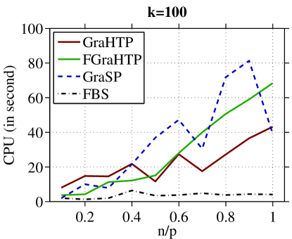
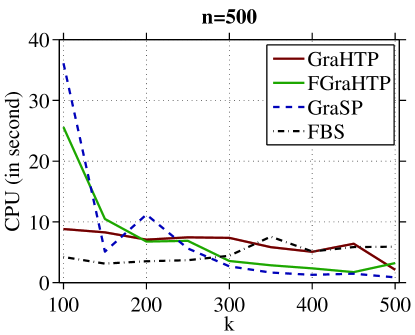
(b) CPU Running Time

Figure 5.1: Simulation data: estimation error and CPU time of the considered algorithms.

5.1.2 Real Data

The algorithms are also compared on the rcv1.binary dataset ($p$ = 47,236) which is a popular dataset for binary classification on sparse data. A training subset of size $n$ = 20,242 and a testing subset of size 20,000 are used. We test with sparsity parameters $k\in\{100,200,...,1000\}$ and fix the regularization parameter $\lambda=10^{-5}$. The initial vector is $w^{(0)}=0$ for all the considered algorithms. We set the stopping criterion as $\|w^{(t)}-w^{(t-1)}\|/\|w^{(t-1)}\|\leq 10^{-4}$ or the iteration stamp $t>50$.

Figure 5.2 shows the evolving curves of empirical logistic loss for $k=200,400,800,1000$. It can be observed from this figure that GraHTP and GraSP are comparable in terms of convergence rate and they are superior to FGraHTP and FBS. The testing classification errors and CPU running time of the considered algorithms are provided in Figure 5.3: (i) in terms of accuracy, all the considered methods are comparable; and (ii) in terms of running time, FGraHTP is the most efficient one; GraHTP is significantly faster than GraSP and FBS. The reason that FGraHTP runs fastest is because it has very low per-iteration cost although its convergence curve is slightly less sharper than GraHTP and GraSP (see Figure 5.2). To summarize, GraHTP and FGraHTP achieve better trade-offs between accuracy and efficiency than GraHTP and FBS on rcv1.binary dataset.

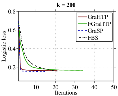
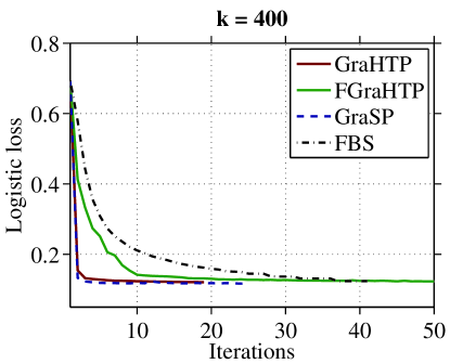
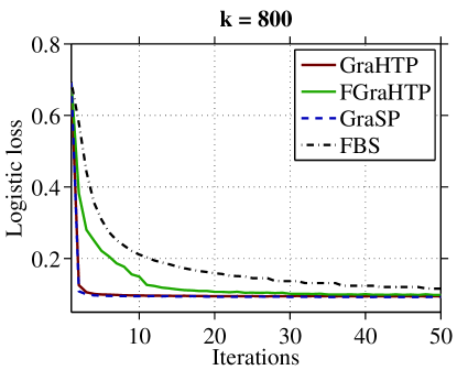
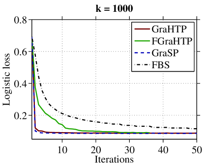
Figure 5.2: rcv1.binary data: $\ell_{2}$-regularized logistic loss vs. number of iterations.

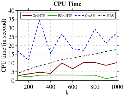
Figure 5.3: rcv1.binary data: Classification error and CPU running time curves of the considered methods.

5.2 Sparsity-Constrained Precision Matrix Estimation

5.2.1 Monte-Carlo Simulation

Our simulation study employs the sparse precision matrix model $\bar{\Omega}=B+\sigma I$ where each off-diagonal entry in $B$ is generated independently and equals 1 with probability $P=0.1$ or 0 with probability $1-P=0.9$. $B$ has zeros on the diagonal, and $\sigma$ is chosen so that the condition number of $\bar{\Omega}$ is $p$. We generate a training sample of size $n=100$ from $\mathcal{N}(0,\bar{\Sigma})$, and an independent sample of size 100 from the same distribution for tuning the parameter $k$. We compare performance for different values of $p\in\{30,60,120,200\}$, replicated 100 times each.

We compare the modified GraHTP (see Algorithm 2) with GraSP and FBS. To adopt GraSP to sparse precision matrix estimation, we modify the algorithm with a similar two-stage strategy as used in the modified GraHTP such that it can handle the eigenvalue bounding constraint in addition to the sparsity constraint. In the work of Yuan & Yan (2013), FBS has already been applied to sparse precision matrix estimation. Also, we compare GraHTP with GLasso (Graphical Lasso) which is a representative convex method for $\ell_{1}$-penalized log-determinant program (Friedman et al., 2008). The quality of precision matrix estimation is measured by its distance to the truth in Frobenius norm and the support recovery F-score. The larger the F-score, the better the support recovery performance. The numerical values over $10^{-3}$ in magnitude are considered to be nonzero.

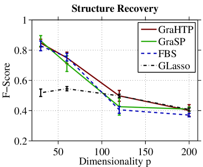
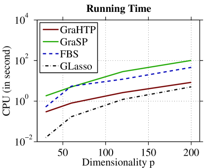
Figure 5.4: Simulated data: comparison of Matrix Frobenius norm loss, support recovery F-score and CPU running time of the considered methods.

Figure 5.4 compares the matrix error in Frobenius norm, sparse recovery F-score and CPU running time achieved by each of the considered algorithms for different $p$. The results show that GraHTP performs favorably in terms of estimation error and support recovery accuracy. We note that the standard errors of GraHTP is relatively larger than Glasso. This is as expected since GraHTP approximately solves a non-convex problem via greedy selection at each iteration; the procedure is less stable than convex methods such as GLasso. Similar phenomenon of instability is observed for GraSP and FBS. Figure 5.4 shows the computational time of the considered algorithms. We observed that GLasso, as a convex solver, is computationally superior to the three considered greedy selection methods. Although inferior to GLasso, GraHTP is computationally much more efficient than GraSP and FBS.

To visually inspect the support recovery performance of the considered algorithms, we show in Figure 5.5 the heatmaps corresponding to the percentage of each matrix entry being identified as a nonzero element with $p=60$. Visual inspection on these heatmaps shows that the three greedy selection methods, GraHTP, GraSP, FBS, tend to be sparser than GLasso. Similar phenomenon is observed in our experiments with other values of $p$.

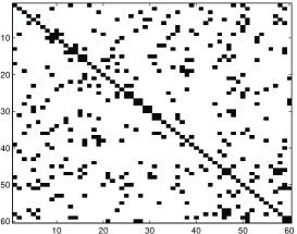
(a) Ground truth

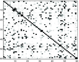
(b) GraHTP

(c) GraSP

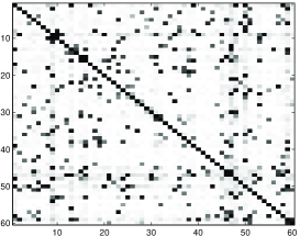
(d) FBS

(e) GLasso

Figure 5.5: Simulation data with $p=60$: heatmaps of the frequency of each precision matrix entry being identified as nonzeros out of 100 replications.

5.2.2 Real Data

We consider the task of LDA (linear discriminant analysis) classification of tumors using the breast cancer dataset (Hess et al., 2006). This dataset consists of 133 subjects, each of which is associated with 22,283 gene expression levels. Among these subjects, 34 are with pathological complete response (pCR) and 99 are with residual disease (RD). The pCR subjects are considered to have a high chance of cancer free survival in the long term. Based on the estimated precision matrix of the gene expression levels, we apply LDA to predict whether a subject can achieve the pCR state or the RD state.

In our experiment, we follow the same protocol used by (Cai et al., 2011) as well as references therein. For the sake of readers, we briefly review this experimental setup. The data are randomly divided into the training and testing sets. In each random division, 5 pCR subjects and 16 RD subjects are randomly selected to constitute the testing data, and the remaining subjects form the training set with size $n=112$. By using two-sample $t$ test, $p=113$ most significant genes are selected as covariates. Following the LDA framework, we assume that the normalized gene expression data are normally distributed as $\mathcal{N}(\mu_{l},\bar{\Sigma})$, where the two classes are assumed to have the same covariance matrix, $\bar{\Sigma}$, but different means, $\mu_{l}$, $l=1$ for pCR state and $l=2$ for RD state. Given a testing data sample $x$, we calculate its LDA scores, $\delta_{l}(x)=x^{\top}\hat{\Omega}{\hat{\mu}}_{l}-\frac{1}{2}{\hat{\mu}}_{l}^{\top}\hat{\Omega}{\hat{\mu}}_{l}+\log{\hat{\pi}}_{l}$, $l=1,2$, using the precision matrix $\hat{\Omega}$ estimated by the considered methods. Here $\hat{\mu}_{l}=(1/n_{l})\sum_{i\in\text{class}_{l}}x_{i}$ is the within-class mean in the training set and ${\hat{\pi}}_{l}=n_{l}/n$ is the proportion of class $l$ subjects in the training set. The classification rule is set as $\hat{l}(x)=\mathop{\arg\max}_{l=1,2}\delta_{l}(x)$. Clearly, the classification performance is directly affected by the estimation quality of $\hat{\Omega}$. Hence, we assess the precision matrix estimation performance on the testing data and compare (modified) GraHTP with GraSP and FBS. We also compare GraHTP with GLasso (Graphical Lasso) (Friedman et al., 2008). We use a 6-fold cross-validation on the training data for tuning $k$. We repeat the experiment 100 times.

Results. To compare the classification performance, we use specificity, sensitivity (or recall), and Mathews correlation coefficient (MCC) criteria as in (Cai et al., 2011):

$$\text{Specificity}=\frac{\text{TN}}{\text{TN}+\text{FP}},\hskip 21.68121pt\text{Sensitivity}=\frac{\text{TP}}{\text{TP}+\text{FN}},$$

$$\text{MCC}=\frac{\text{TP}\times\text{TN}-\text{FP}\times\text{FN}}{\sqrt{(\text{TP}+\text{FP})(\text{TP}+\text{FN})(\text{TN}+\text{FP})(\text{TN}+\text{FN})}},$$

where TP and TN stand for true positives (pCR) and true negatives (RD), respectively, and FP and FN stand for false positives/ negatives, respectively. The larger the criterion value, the better the classification performance. Since one can adjust decision threshold in any specific algorithm to trade-off specificity and sensitivity (increase one while reduce the other), the MCC is more meaningful as a single performance metric.

Table 5.1: Brease cancer data: comparison of average (std) classification accuracy and average CPU running time over 100 replications.

Methods	Specificity	Sensitivity	MCC	CPU Time (sec.)
GraHTP	0.77 (0.11)	0.77 (0.19)	0.49 (0.19)	1.92
GraSP	0.73 (0.10)	0.78 (0.18)	0.45 (0.17)	4.06
FBS	0.78 (0.11)	0.74 (0.18)	0.48 (0.19)	8.73
GLasso	0.81 (0.11)	0.64 (0.21)	0.45 (0.19)	1.19

Table 5.1 reports the averages and standard deviations, in the parentheses, of the three classification criteria over 100 replications. It can be observed that GraHTP is quite competitive to the leading methods in terms of the three metrics. The averages of CPU running time (in seconds) of the considered methods are listed in the last column of Table 5.1. Figure 5.6 shows the evolving curves of log-determinant loss verses number of iterations. We observed that on this data, GraHTP converges much faster than GraSP and FBS. Note that we did not draw the curve of GLasso in Figure 5.6 because its objective function is different from that of the problem (4.6).

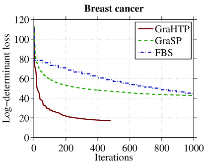
Figure 5.6: Brease cancer data: log-determinant loss convergence curves of the considered methods.

6 Conclusion

In this paper, we propose GraHTP as a generalization of HTP from compressive sensing to the generic problem of sparsity-constrained optimization. The main idea is to force the gradient descent iteration to be sparse via hard threshloding. Theoretically, we prove that under mild conditions, GraHTP converges geometrically in finite steps of iteration and its estimation error is controlled by the restricted norm of gradient at the target sparse solution. We also propose and analyze the FGraHTP algorithm as a fast variant of GraHTP without the debiasing step. Empirically, we compare GraHTP and FGraHTP with several representative greedy selection methods when applied to sparse logistic regression and sparse precision matrix estimation tasks. Our theoretical results and empirical evidences show that simply combing gradient descent with hard threshloding, with or without debiasing, leads to efficient and accurate computational procedures for sparsity-constrained optimization problems.

Appendix A Technical Proofs

A.1 Proof of Lemma 1

Proof.

Part (a): The first inequality follows from the triangle inequality. The second inequality can be derived by combining the first one and the integration $f(x)-f(y)-\langle\nabla f(y),x-y\rangle=\int_{0}^{1}\langle\nabla f(y+\tau(x-y))-\nabla f(y),x-y\rangle d\tau$.

Part (b): By adding two copies of the inequality (3.1) with $x$ and $y$ interchanged and using the Theorem 2.1.5 in (Nesterov, 2004), we know that

$$(x-y)^{\top}(\nabla f(x)-\nabla f(y))\geq m_{s}\|x-y\|^{2},\quad\|\nabla_{F}f(x)-\nabla_{F}f(y)\|\leq M_{s}\|x-y\|.$$

For any $\zeta>0$ we have

$$\|x-y-\zeta\nabla_{F}f(x)+\zeta\nabla_{F}f(y)\|^{2}\leq(1-2\zeta m_{s}+\zeta^{2}M_{s}^{2})\|x-y\|^{2}.$$

If $\zeta<2m_{s}/M^{2}_{s}$, then $\rho_{s}=\sqrt{1-2\zeta m_{s}+\zeta^{2}M_{s}^{2}}<1$. This proves the desired result. ∎

A.2 Proof of Theorem 1

Proof.

We first prove the finite iteration guarantee of GraHTP. Let us consider the vector $\tilde{x}^{(t)}_{k}$ which is the restriction of $\tilde{x}^{(t)}$ on $F^{(t)}$. According to the definition of $x^{(t)}$ we have $f(x^{(t)})\leq f(\tilde{x}^{(t)}_{k})$. It follows that

$$f(x^{(t)})-f(x^{(t-1)}) \leq f(\tilde{x}^{(t)}_{k})-f(x^{(t-1)})$$ (A.1)

$$\leq \langle\nabla f(x^{(t-1)}),\tilde{x}^{(t)}_{k}-x^{(t-1)}\rangle+\frac{1+\rho_{2k}}{2\zeta}\|\tilde{x}^{(t)}_{k}-x^{(t-1)}\|^{2}$$

$$\leq -\frac{1}{2\eta}\|\tilde{x}^{(t)}_{k}-x^{(t-1)}\|^{2}+\frac{1+\rho_{2k}}{2\zeta}\|\tilde{x}^{(t)}_{k}-x^{(t-1)}\|^{2}$$

$$= -\frac{\zeta-\eta(1+\rho_{2k})}{2\zeta\eta}\|\tilde{x}^{(t)}_{k}-x^{(t-1)}\|^{2},$$

where the second inequality follows from Lemma 1 and the third inequality follows from the fact that $\tilde{x}^{(t)}_{k}$ is a better $k$-sparse approximation to $\tilde{x}^{(t)}$ than $x^{(t-1)}$ so that $\|\tilde{x}^{(t)}_{k}-\tilde{x}^{(t)}\|=\|\tilde{x}^{(t)}_{k}-x^{(t-1)}+\eta\nabla f(x^{(t-1)})\|^{2}\leq\|x^{(t-1)}-x^{(t-1)}+\eta\nabla f(x^{(t-1)})\|^{2}=\|\eta\nabla f(x^{(t-1)})\|^{2}$, which implies $2\eta\langle\nabla f(x^{(t-1)}),\tilde{x}^{(t)}_{k}-x^{(t-1)}\rangle\leq-\|\tilde{x}^{(t)}_{k}-x^{(t-1)}\|^{2}$. Since $\eta(1+\rho_{2k})<\zeta$, it follows that the sequence $\{f(x^{(t)})\}$ is nonincreasing, hence it is convergent. Since it is also eventually periodic, it must be eventually constant. In view of (A.1), we deduce that $\tilde{x}^{(t)}_{k}=x^{(t-1)}$, and in particular that $F^{(t)}=F^{(t-1)}$, for $t$ large enough. This implies that $x^{(t)}=x^{(t-1)}$ for $t$ large enough, which implies the desired result.

By noting that $x^{(t)}=\tilde{x}^{(t)}_{k}$ and from the inequality (A.1), we immediately establish the convergence of the sequence $\{f(x^{(t)})\}$ defined by FGraHTP. ∎

A.3 Proof of Theorem 2

Proof.

Part (a): The first step of the proof is a consequence of the debiasing step S3. Since $x^{(t)}$ is the minimum of $f(x)$ restricted over the supporting set $F^{(t)}$, we have $\langle\nabla f(x^{(t)}),z\rangle=0$ whenever $\text{supp}(z)\subseteq F^{(t)}$. Let $\bar{F}=\text{supp}(\bar{x})$ and $F=\bar{F}\cup F^{(t)}\cup F^{(t-1)}$. It follows that

$$\|(x^{(t)}-\bar{x})_{F^{(t)}}\|^{2} = \langle x^{(t)}-\bar{x},(x^{(t)}-\bar{x})_{F^{(t)}}\rangle$$

$$= \langle x^{(t)}-\bar{x}-\zeta\nabla_{F^{(t)}}f(x^{(t)})+\zeta\nabla_{F^{(t)}}f(\bar{x}),(x^{(t)}-\bar{x})_{F^{(t)}}\rangle-\zeta\langle\nabla_{F^{(t)}}f(\bar{x}),(x^{(t)}-\bar{x})_{F^{(t)}}\rangle$$

$$\leq \rho_{s}\|x^{(t)}-\bar{x}\|\|(x^{(t)}-\bar{x})_{F^{(t)}}\|+\zeta\|\nabla_{k}f(\bar{x})\|\|(x^{(t)}-\bar{x})_{F^{(t)}}\|,$$

where the last inequality is from Condition $C(s,\zeta,\rho_{s})$, $\rho_{k+\bar{k}}\leq\rho_{s}$ and $\|\nabla_{F^{(t)}}f(\bar{x})\|\leq\|\nabla_{k}f(\bar{x})\|$. After simplification, we have $\|(x^{(t)}-\bar{x})_{F^{(t)}}\|\leq\rho_{s}\|x^{(t)}-\bar{x}\|+\zeta\|\nabla_{k}f(\bar{x})\|$. It follows that

$$\|x^{(t)}-\bar{x}\|\leq\|(x^{(t)}-\bar{x})_{F^{(t)}}\|+\|(x^{(t)}-\bar{x})_{\overline{F^{(t)}}}\|\leq\rho_{s}\|x^{(t)}-\bar{x}\|+\zeta\|\nabla_{k}f(\bar{x})\|+\|(x^{(t)}-\bar{x})_{\overline{F^{(t)}}}\|.$$

After rearrangement we obtain

$$\|x^{(t)}-\bar{x}\|\leq\frac{\|(x^{(t)}-\bar{x})_{\overline{F^{(t)}}}\|}{1-\rho_{s}}+\frac{\zeta\|\nabla_{k}f(\bar{x})\|}{1-\rho_{s}}.$$ (A.2)

The second step of the proof is a consequence of steps S1 and S2. We notice that

$$\|(x^{(t-1)}-\eta\nabla f(x^{(t-1)}))_{\bar{F}}\|\leq\|(x^{(t-1)}-\eta\nabla f(x^{(t-1)}))_{F^{(t)}}\|.$$

By eliminating the contribution on $\bar{F}\cap F^{(t)}$, we derive

$$\|(x^{(t-1)}-\eta\nabla f(x^{(t-1)}))_{\bar{F}\backslash F^{(t)}}\|\leq\|(x^{(t-1)}-\eta\nabla f(x^{(t-1)}))_{F^{(t)}\backslash\bar{F}}\|.$$

For the right-hand side, we have

$$\|(x^{(t-1)}-\eta\nabla f(x^{(t-1)}))_{F^{(t)}\backslash\bar{F}}\|\leq\|(x^{(t-1)}-\bar{x}-\eta\nabla f(x^{(t-1)})+\eta\nabla f(\bar{x}))_{F^{(t)}\backslash\bar{F}}\|+\eta\|\nabla_{k}f(\bar{x})\|.$$

As for the left-hand side, we have

$$\|(x^{(t-1)}-\eta\nabla f(x^{(t-1)}))_{\bar{F}\backslash F^{(t)}}\|$$

$$\geq \|(x^{(t-1)}-\bar{x}-\eta\nabla f(x^{(t-1)})+\eta\nabla f(\bar{x}))_{\bar{F}\backslash F^{(t)}}+(x^{(t)}-\bar{x})_{\overline{F^{(t)}}}\|-\eta\|\nabla_{k}f(\bar{x})\|$$

$$\geq \|(x^{(t)}-\bar{x})_{\overline{F^{(t)}}}\|-\|(x^{(t-1)}-\bar{x}-\eta\nabla f(x^{(t-1)})+\eta\nabla f(\bar{x}))_{\bar{F}\backslash F^{(t)}}\|-\eta\|\nabla_{k}f(\bar{x})\|.$$

With $\bar{F}\Delta F^{(t)}$ denoting the symmetric difference of the set $\bar{F}$ and $F^{(t)}$, it follows that

$$\|(x^{(t)}-\bar{x})_{\overline{F^{(t)}}}\|$$ (A.3)

$$\leq \sqrt{2}\|(x^{(t-1)}-\bar{x}-\eta\nabla f(x^{(t-1)})+\eta\nabla f(\bar{x}))_{\bar{F}\Delta F^{(t)}}\|+2\eta\|\nabla_{k}f(\bar{x})\|$$

$$\leq \sqrt{2}\|x^{(t-1)}-\bar{x}-\eta\nabla_{F}f(x^{(t-1)})+\eta\nabla_{F}f(\bar{x})\|+2\eta\|\nabla_{k}f(\bar{x})\|$$

$$\leq \sqrt{2}\|x^{(t-1)}-\bar{x}-\zeta\nabla_{F}f(x^{(t-1)})+\zeta\nabla_{F}f(\bar{x})\|+\sqrt{2}(\zeta-\eta)\|\nabla_{F}f(x^{(t-1)})-\nabla_{F}f(\bar{x})\|+2\eta\|\nabla_{k}f(\bar{x})\|$$

$$\leq \sqrt{2}(1-\eta/\zeta+(2-\eta/\zeta)\rho_{s})\|x^{(t-1)}-\bar{x}\|+2\eta\|\nabla_{k}f(\bar{x})\|,$$

where the last inequality follows from Condition $C(s,\zeta,\rho_{s})$, $\eta<\zeta$ and Lemma 1. As a final step, we put (A.2) and (A.3) together to obtain

$$\|x^{(t)}-\bar{x}\|\leq\frac{\sqrt{2}(1-\eta/\zeta+(2-\eta/\zeta)\rho_{s})}{1-\rho_{s}}\|x^{(t-1)}-\bar{x}\|+\frac{(2\eta+\zeta)\|\nabla_{k}f(\bar{x})\|}{1-\rho_{s}}$$

Since $\mu_{1}=\sqrt{2}(1-\eta/\zeta+(2-\eta/\zeta)\rho_{s})/(1-\rho_{s})<1$, by recursively applying the above inequality we obtain the desired inequality in part (a).

Part (b): Recall that $F^{(t)}=\text{supp}(x^{(t)},k)$ and $F=F^{(t-1)}\cup F^{(t)}\cup\text{supp}(\bar{x})$. Consider the following vector

$$y=x^{(t-1)}-\eta\nabla_{F}f(x^{(t-1)}).$$

By using triangular inequality we have

$$\|y-\bar{x}\| = \|x^{(t-1)}-\eta\nabla_{F}f(x^{(t-1)})-\bar{x}\|$$

$$\leq \|x^{(t-1)}-\bar{x}-\eta\nabla_{F}f(x^{(t-1)})+\eta\nabla_{F}f(\bar{x})\|+\eta\|\nabla_{F}f(\bar{x})\|$$

$$\leq (1-\eta/\zeta+(2-\eta/\zeta)\rho_{s})\|x^{(t-1)}-\bar{x}\|+\eta\|\nabla_{s}f(\bar{x})\|,$$

where the last inequality follows from Condition $C(s,\zeta,\rho_{s})$, $\eta<\zeta$ and $\|\nabla_{F}f(\bar{x})\|\leq\|\nabla_{s}f(\bar{x})\|$. For FGraHTP, we note that $x^{(t)}=\tilde{x}^{(t)}_{k}=y_{k}$, and thus $\|x^{(t)}-\bar{x}\|\leq\|x^{(t)}-y\|+\|y-\bar{x}\|\leq 2\|y-\bar{x}\|$. It follows that

$$\|x^{(t)}-\bar{x}\|\leq 2(1-\eta/\zeta+(2-\eta/\zeta)\rho_{s})\|x^{(t-1)}-\bar{x}\|+2\eta\|\nabla_{s}f(\bar{x})\|.$$

Since $\mu_{2}=2(1-\eta/\zeta+(2-\eta/\zeta)\rho_{s})<1$, by recursively applying the above inequality we obtain the desired inequality in part (b). ∎

A.4 Proof of Proposition 1

Proof.

Obviously, $f(w)$ is $\lambda$-strongly convex. Consider an index set $F$ with cardinality $|F|\leq s$ and all $w,w^{\prime}$ with $\text{supp}(w)\cup\text{supp}(w^{\prime})\subseteq F$. Since $\sigma(z)$ is Lipschitz continuous with constant $1$, we have

$$|[a(w)]_{i}-[a(w^{\prime})]_{i})| = 2|\sigma(2v^{(i)}w^{\top}u^{(i)})-\sigma(2v^{(i)}w^{\prime\top}u^{(i)})|$$

$$\leq 4|(w-w^{\prime})^{\top}v^{(i)}u^{(i)}|$$

$$\leq 4\|(u^{(i)})_{F}\|\|w-w^{\prime}\|$$

$$\leq 4R_{s}\|w-w^{\prime}\|,$$

which implies

$$\|a(w)-a(w^{\prime})\|_{\infty}\leq 4R_{s}\|w-w^{\prime}\|.$$

Therefore we have

$$\|\nabla_{F}f(w)-\nabla_{F}f(w^{\prime})\| \leq \frac{1}{n}\|U_{F\bullet}(a(w)-a(w^{\prime}))\|+\lambda\|w-w^{\prime}\|$$

$$\leq \frac{1}{n}\|U_{F\bullet}(a(w)-a(w^{\prime}))\|_{1}+\lambda\|w-w^{\prime}\|$$

$$\leq \frac{1}{n}|U_{F\bullet}|_{1}\|a(w)-a(w^{\prime})\|_{\infty}+\lambda\|w-w^{\prime}\|$$

$$\leq (4\sqrt{s}R_{s}^{2}+\lambda)\|w-w^{\prime}\|,$$

where the second “$\leq$” follows $\|x\|\leq\|x\|_{1}$, the third “$\leq$” follows from $\|Ax\|_{1}\leq|A|_{1}\|x\|_{\infty}$, and last “$\leq$” follows from $|U_{F\bullet}|_{1}\leq n\sqrt{s}\max_{i}\|[u^{(i)}]_{F}\|\leq n\sqrt{s}R_{s}$. Therefore $f$ is $(4\sqrt{s}R_{s}^{2}+\lambda)$-strongly smooth. The desired result follows directly from Part(b) of Lemma 1. ∎

A.5 Proof of Proposition 2

Proof.

For any index set $F$ with $|F|\leq s$, we can deduce

$$\|\nabla_{F}f(\bar{w})\| \leq \|[\nabla l(\bar{w})]_{F}\|+\lambda\|\bar{w}_{F}\|\leq\sqrt{s}\|\nabla l(\bar{w})\|_{\infty}+\lambda\|\bar{w}_{s}\|.$$ (A.4)

We next bound the term $\|\nabla l(\bar{w})\|_{\infty}$. From (4.4) we have

$$\left|\frac{\partial l}{\partial[\bar{w}]_{j}}\right| = \left|\frac{1}{n}\sum_{i=1}^{n}-v^{(i)}[u^{(i)}]_{j}+\mathbb{E}_{v}[v[u^{(i)}]_{j}\mid u^{(i)}]\right|$$

$$\leq \left|\frac{1}{n}\sum_{i=1}^{n}v^{(i)}[u^{(i)}]_{j}-\mathbb{E}[v[u]_{j}]\right|+\left|\frac{1}{n}\sum_{i=1}^{n}\mathbb{E}_{v}[v[u^{(i)}]_{j}\mid u^{(i)}]-\mathbb{E}[v[u]_{j}]\right|,$$

where $\mathbb{E}[]$ is taken over the distribution (4.3). Therefore, for any $\varepsilon>0$,

$$\mathbb{P}\left(\left|\frac{\partial l}{\partial[\bar{w}]_{j}}\right|>\varepsilon\right) \leq \mathbb{P}\left(\left|\frac{1}{n}\sum_{i=1}^{n}v^{(i)}[u^{(i)}]_{j}-\mathbb{E}[v[u]_{j}]\right|>\frac{\varepsilon}{2}\right)$$

$$+\mathbb{P}\left(\left|\frac{1}{n}\sum_{i=1}^{n}\mathbb{E}_{v}[v[u^{(i)}]_{j}\mid u^{(i)}]-\mathbb{E}[v[u]_{j}]\right|>\frac{\varepsilon}{2}\right)$$

$$\leq 4\exp\left\{-\frac{n\varepsilon^{2}}{8\sigma^{2}}\right\},$$

where the last “$\leq$” follows from the large deviation inequality of sub-Gaussian random variables which is standard (see, e.g., Vershynin, 2011). By the union bound we have

$$\mathbb{P}(\|\nabla l(\bar{w})\|_{\infty}>\varepsilon) \leq 4p\exp\left\{-\frac{n\varepsilon^{2}}{8\sigma^{2}}\right\}.$$

By letting $\varepsilon=4\sigma\sqrt{\ln p/n}$, we know that with probability at least $1-4p^{-1}$,

$$\|\nabla l(\bar{w})\|_{\infty}\leq 4\sigma\sqrt{\ln p/n}.$$

Combing the above inequality with (A.4) yields the desired result. ∎

Appendix B Solving Subproblem (4.7) via ADM

In this appendix section, we provide our implementation details of ADM for solving the subproblem (4.7). By introducing an auxiliary variable $\Theta\in\mathbb{R}^{p\times p}$, the problem (4.7) is obviously equivalent to the following problem:

$$\min_{\alpha I\preceq\Omega\preceq\beta I}L(\Omega),\ \ \ \text{s.t. }\Omega=\Theta,\text{supp}(\Theta)\subseteq F.$$ (B.1)

Then, the Augmented Lagrangian function of (B.1) is

$$J(\Omega,\Theta,\Gamma):=L(\Omega)-\langle\Gamma,\Omega-\Theta\rangle+\frac{\rho}{2}\|\Omega-\Theta\|_{Frob}^{2},$$

where $\Gamma\in\mathbb{R}^{p\times p}$ is the multiplier of the linear constraint $\Omega=\Theta$ and $\rho>0$ is the penalty parameter for the violation of the linear constraint. The ADM solves the following problems to generate the new iterate:

$$\Omega^{(\tau+1)} = \mathop{\arg\min}_{\alpha I\preceq\Omega\preceq\beta I}J(\Omega,\Theta^{(\tau)},\Gamma^{(\tau)}),$$ (B.2)

$$\Theta^{(\tau+1)} = \mathop{\arg\min}_{\text{supp}(\Theta)\subseteq F}J(\Omega^{(\tau+1)},\Theta,\Gamma^{(\tau)}),$$ (B.3)

$$\Gamma^{(\tau+1)} = \Gamma^{(\tau)}-\rho(\Omega^{(\tau+1)}-\Theta^{(\tau+1)}).$$

Let us first consider the minimization problem (B.2). It is easy to verify that it is equivalent to the following minimization problem:

$$\Omega^{(\tau+1)}=\mathop{\arg\min}_{\alpha I\preceq\Omega\preceq\beta I}\frac{1}{2}\left\|\Omega-M\right\|_{Frob}^{2}-\frac{1}{\rho}\log\det\Omega,$$

where

$$M=\Theta^{(\tau)}-\frac{1}{\rho}(\Sigma_{n}-\Gamma^{(\tau)}).$$

Let the singular value decomposition of $M$ be

$$M=V\Lambda V^{\top},\ \ \text{ with }\Lambda=\text{diag}(\lambda_{1},...,\lambda_{n}).$$

It is easy to verify that the solution of problem (B.2) is given by

$$\Omega^{(\tau+1)}=V\tilde{\Lambda}V^{\top},\ \ \text{ with }\tilde{\Lambda}=\text{diag}(\tilde{\lambda}_{1},...,\tilde{\lambda}_{n}),$$

where

$$\tilde{\lambda}_{j}=\min\left\{\beta,\max\left\{\alpha,\frac{\lambda_{j}+\sqrt{\lambda_{j}^{2}+4/\rho}}{2}\right\}\right\}.$$

Next, we consider the minimization problem (B.3). It is straightforward to see that the solution of problem (B.3) is given by

$$\Theta^{(\tau+1)}=\left[\Omega^{(\tau+1)}-1/\rho\Gamma^{(\tau)}\right]_{F}.$$

References

- Agarwal et al. (2010) Agarwal, A., Negahban, S., and Wainwright, M. Fast global convergence rates of gradient methods for high-dimensional statistical recovery. In Proceedings of the 24th Annual Conference on Neural Information Processing Systems (NIPS’10), 2010.
- Bahmani et al. (2013) Bahmani, S., Raj, B., and Boufounos, P. Greedy sparsity-constrained optimization. Journal of Machine Learning Research, 14:807–841, 2013.
- Beck & Teboulle (2009) Beck, A. and Teboulle, Marc. A fast iterative shrinkage-thresholding algorithm for linear inverse problems. SIAM Journal on Imaging Sciences, 2(1):183–202, 2009.
- Bishop (2006) Bishop, C.M. Pattern Recognition and Machine Learning. Springer-Verlag New York, Inc., Secaucus, NJ, USA, 2006. ISBN 978-0-387-31073-2.
- Blumensath & Davies (2009) Blumensath, T. and Davies, M. E. Iterative hard thresholding for compressed sensing. Applied and Computational Harmonic Analysis, 27(3):265–274, 2009.
- Boyd et al. (2010) Boyd, S., Parikh, N., Chu, E., Peleato, B., and Eckstein, J. Distributed optimization and statistical learning via the alternating direction method of multipliers. Foundations and Trends in Machine Learning, 3:1–122, 2010.
- Cai et al. (2011) Cai, T., liu, W., and Luo, X. A constrained minimization approach to sparse precision matrix estimation. Journal of the American Statistical Association, 106(494):594–607, 2011.
- Candès et al. (2006) Candès, E. J., Romberg, J. K., and Tao, T. Stable signal recovery from incomplete and inaccurate measurements. Communications on Pure and Applied Mathematics, 59(8):1207–1223, 2006.
- Dai & Milenkovic (2009) Dai, W. and Milenkovic, O. Subspace pursuit for compressive sensing signal reconstruction. IEEE Transactions on Information Theory, 55(5):2230–2249, 2009.
- Donoho (2006) Donoho, D. L. Compressed sensing. IEEE Transactions on Information Theory, 52(4):1289–1306, 2006.
- Edwards (2000) Edwards, D. M. Introduction to Graphical Modelling. Springer, New York, 2000.
- Foucart (2011) Foucart, S. Hard thresholding pursuit: An algorithm for compressive sensing. SIAM Journal on Numerical Analysis, 49(6):2543–2563, 2011.
- Foucart (2012) Foucart, S. Sparse recovery algorithms: sufficient conditions in terms of restricted isometry constants. In Approximation Theory XIII: San Antonio 2010, volume 13 of Springer Proceedings in Mathematics, pp. 65–77, 2012.
- Frank & Wolfe (1956) Frank, M. and Wolfe, P. An algorithm for quadratic programming. Naval Res. Logist. Quart., 5:95–110, 1956.
- Friedman et al. (2008) Friedman, J., Hastie, T., and Tibshirani, R. Sparse inverse covariance estimation with the graphical lasso. Biostatistics, 9(3):432–441, 2008.
- Hess et al. (2006) Hess, K. R., Anderson, K., Symmans, W. F., and et al. Pharmacogenomic predictor of snesitivity to preoperative chemotherapy with paclitaxel and fluorouracil, doxorubicin, and cyclophosphamide in breast cancer. Journal of Clinical Oncology, 24:4236–4244, 2006.
- Jaggi (2011) Jaggi, M. Sparse convex optimization methods for machine learning. Technical report, PhD thesis in Theoretical Computer Science, ETH Zurich, 2011.
- Jalali et al. (2011) Jalali, A., Johnson, C. C., and Ravikumar, P. K. On learning discrete graphical models using greedy methods. In Proceedings of the 25th Annual Conference on Neural Information Processing Systems (NIPS’11), 2011.
- Kim & Kim (2004) Kim, Yongdai and Kim, Jinseog. Gradient lasso for feature selection. In Proceedings of the Twenty-first International Conference on Machine Learning (ICML’04), pp. 60–67, 2004.
- Lu (2009) Lu, Z. Smooth optimization approach for sparse covariance selection. SIAM Journal on Optimization, 19(4):1807–1827, 2009.
- Ma (2013) Ma, Z. Sparse principal component analysis and iterative thresholding. Annals of Statistics, 41(2):772–801, 2013.
- Mallat & Zhang (1993) Mallat, S. and Zhang, Zhifeng. Matching pursuits with time-frequency dictionaries. IEEE Transactions on Signal Processing, 41(12):3397–3415, 1993.
- Natarajan (1995) Natarajan, B. K. Sparse approximate solutions to linear systems. SIAM Journal on Computing, 24(2):227–234, 1995.
- Needell & Tropp (2009) Needell, D. and Tropp, J. A. Cosamp: iterative signal recovery from incomplete and inaccurate samples. IEEE Transactions on Information Theory, 26(3):301–321, 2009.
- Nesterov (2004) Nesterov, Y. Introductory Lectures on Convex Optimization: A Basic Course. Kluwer, 2004. ISBN 978-1402075537.
- Ravikumar et al. (2011) Ravikumar, P., Wainwright, M. J., Raskutti, G., and Yu, B. High-dimensional covariance estimation by minimizing -penalized log-determinant divergence. Electronic Journal of Statistics, 5:935–980, 2011.
- Shalev-Shwartz et al. (2010) Shalev-Shwartz, Shai, Srebro, Nathan, and Zhang, Tong. Trading accuracy for sparsity in optimization problems with sparsity constraints. SIAM Journal on Optimization, 20:2807–2832, 2010.
- Tewari et al. (2011) Tewari, A., Ravikumar, P., and Dhillon, I. S. Greedy algorithms for structurally constrained high dimensional problems. In Proceedings of the 25th Annual Conference on Neural Information Processing Systems (NIPS’11), 2011.
- Tropp & Gilbert (2007) Tropp, J. and Gilbert, A. Signal recovery from random measurements via orthogonal matching pursuit. IEEE Transactions on Information Theory, 53(12):4655–4666, 2007.
- Vershynin (2011) Vershynin, Roman. Introduction to the non-asymptotic analysis of random matrices. 2011. URL http://arxiv.org/pdf/1011.3027.pdf.
- Wainwright & Jordan (2008) Wainwright, M.J. and Jordan, M.I. Graphical models, exponential families, and variational inference. Foundations and Trends in Machine Learning, 1(1-2):1–305, 2008.
- Yuan (2012) Yuan, X. M. Alternating direction method of multipliers for covariance selection models. Journal of Scientific Computing, 51:261–273, 2012.
- Yuan & Yan (2012) Yuan, X.-T. and Yan, S. Forward basis selection for sparse approximation over dictionary. In Proceedings of the Fifteenth International Conference on Artificial Intelligence and Statistics (AISTATS’12), 2012.
- Yuan & Yan (2013) Yuan, X.-T. and Yan, S. Forward basis selection for pursuing sparse representations over a dictionary. IEEE Transactions on Pattern Analysis And Machine Intelligence, 35(12):3025–3036, 2013.
- Yuan & Zhang (2013) Yuan, X.-T. and Zhang, T. Truncated power method for sparse eigenvalue problems. Journal of Machine Learning Research, 14:899–925, 2013.
- Zhang (2008) Zhang, T. Adative forward-backward greedy algorithm for sparse learning with linear models. In Proceedings of the 22nd Annual Conference on Neural Information Processing Systems (NIPS’08), 2008.