Quantum hoop conjecture: Black hole formation by particle collisions

Abstract

We address the issue of (quantum) black hole formation by particle collision in quantum physics. We start by constructing the horizon wave-function for quantum mechanical states representing two highly boosted non-interacting particles that collide in flat one-dimensional space. From this wave-function, we then derive a probability that the system becomes a black hole as a function of the initial momenta and spatial separation between the particles. This probability allows us to extend the hoop conjecture to quantum mechanics and estimate corrections to its classical counterpart.

I Introduction

The general relativistic (GR) description of the gravitational collapse, leading to the formation of black holes (BHs), was first investigated in the seminal papers of Oppenheimer and co-workers OS , but a thorough understanding of the physics of such processes still stands as one of the most challenging issues for contemporary theoretical physics. The literature on the subject has grown immensely (see, e.g. Ref. joshi ), but many technical and conceptual difficulties remain unsolved, particularly if one tries to account for the quantum mechanical (QM) nature of collapsing matter. What is unanimously accepted is that the gravitational interaction becomes important whenever a large enough amount of matter is “compacted” within a sufficiently small volume. K. Thorne formulated this idea in the hoop conjecture Thorne:1972ji , which states that a BH forms if two colliding objects fall within their “black disk”. Assuming the final configuration is (approximately) spherically symmetric, this occurs when the system occupies a sphere whose radius $r$ is smaller than the gravitational Schwarzschild radius,

$$r\lesssim R_{\rm H}\equiv 2\,\ell_{\rm p}\,\frac{E}{m_{\rm p}}\ ,$$ (1)

where $E$ is the total energy in the centre-of-mass frame (see next Section for more details). Note that we use units with $c=1$, the Newton constant $G_{\rm N}=\ell_{\rm p}/m_{\rm p}$, where $\ell_{\rm p}$ and $m_{\rm p}$ are the Planck length and mass, respectively, and $\hbar=\ell_{\rm p}\,m_{\rm p}$ .

The hoop conjecture applies to astrophysical bodies, whose energy is orders of magnitude above the scale of quantum gravity, and can therefore be reasonably described by classical GR joshi ; Thorne:1972ji ; payne ; murchadha . One of the most important questions which then arises is what happens when the total energy of the colliding particles is of the Planck size or less qgc . Just to give this question a precise meaning is a conceptual challenge, because QM effects may hardly be neglected acmo , and the very notion of horizon becomes “fuzzy”. In fact, it was recently proposed in Refs. Casadio to define a wave-function for the horizon, which can be associated with any localised QM particle. The auxiliary wave-function yields the probability of finding a horizon of a certain radius centred around the source, and one can therefore determine the probability that a QM particle is a BH depending on its mass. This probability is found to vanish very fast for particles lighter than the Planck mass, as one expects from qualitative arguments.

We remark that a realistic description of quantum (with $E\simeq m_{\rm p}$) hsu or classical ($E\gg m_{\rm p}$) BHs very likely requires the knowledge of their microscopic structure dvali . We however do not consider such important details here, and just address the conceptual problem of developing a framework which can be used to study the formation of horizons in systems containing QM sources. Of course, a more canonical framework already exists, in principle, and is given by quantum field theory on curved backgrounds coupled to the semiclassical Einstein equations pina . Thereby, one should be able to describe quantum matter states on a sufficiently arbitrary space-time, which is to be determined self-consistently by solving the Einstein equations with the corresponding renormalised matter energy-momentum tensor. Since obtaining the normal modes and building the matter Fock space is in general impossible, this procedure has failed to provide practical estimates so far .

In this work, after reviewing the case of a single spherically symmetric particle, we shall consider two-particle QM states and build their horizon wave-function. This construction will naturally lead to a QM generalisation of the hoop conjecture and specific corrections to its classical formulation (1). It is important to remark from the onset that these results will be obtained analytically, but at the price of making several rather strong simplifying assumptions. In particular, we shall just consider free particles in one spatial dimension, and neglect any space-time curvature.

II Horizon wave-function in spherical symmetry

Inspired by Eq. (1), we can define a horizon wave-function given the QM wave-function of a particle in position space Casadio . The idea stems from the classical GR theory of spherically symmetric systems, for which the metric $g_{\mu\nu}$ can always be written as

$$\mbox{${\rm d}$}s^{2}=g_{ij}\,\mbox{${\rm d}$}x^{i}\,\mbox{${\rm d}$}x^{j}+r^{2}(x^{i})\left(\mbox{${\rm d}$}\theta^{2}+\sin^{2}\theta\,\mbox{${\rm d}$}\phi^{2}\right)\ ,$$ (2)

with $x^{i}=(x^{1},x^{2})$ coordinates on surfaces where the angles $\theta$ and $\phi$ are constant. The location of a trapping horizon, a surface where the escape velocity equals the speed of light, is determined by the equation murchadha

$$0=g^{ij}\,\nabla_{i}r\,\nabla_{j}r=1-\frac{2\,M}{r}\ ,$$ (3)

where $\nabla_{i}r$ is the covector perpendicular to surfaces of constant area $\mathcal{A}=4\,\pi\,r^{2}$. The function $M=\ell_{\rm p}\,m/m_{\rm p}$ is the active (Misner-Sharp) gravitational mass, representing the total energy enclosed within a sphere of radius $r$ and, if we set $x^{1}=t$ and $x^{2}=r$, we find

$$M(t,r)=\frac{4\,\pi\,\ell_{\rm p}}{3\,m_{\rm p}}\int_{0}^{r}\rho(t,\bar{r})\,\bar{r}^{2}\,\mbox{${\rm d}$}\bar{r}\ ,$$ (4)

as if the space inside the sphere were flat.

For elementary particles we know for an experimental fact that QM effects may not be neglected acmo . In fact, the Heisenberg principle of QM introduces an uncertainty in the spatial localisation of a spinless point-like source of mass $m$, typically of the order of the Compton-de Broglie length,

$$\lambda_{m}\simeq\ell_{\rm p}\,{m_{\rm p}}/{m}\ .$$ (5)

Assuming QM is a better description of reality implies that the Schwarzschild radius in Eq. (1) with $E=m$ only makes sense if $R_{\rm H}\gtrsim\lambda_{m}$, or $m\gtrsim m_{\rm p}$ (and $M\gtrsim\ell_{\rm p}$). Note we employed the flat space Compton length (5), which is likely the particle’s self-gravity will affect, but it is still a reasonable order of magnitude estimate, and BHs can therefore only exist with mass (much) larger than the Planck scale.

Let us now consider a QM state $\psi_{\rm S}$ representing a massive particle localised in space and at rest in the chosen reference frame. Having defined suitable Hamiltonian eigenmodes, $\hat{H}\,\mbox{$\mid\psi_{E}\,\rangle$}=E\,\mbox{$\mid\psi_{E}\,\rangle$}$, where $H$ can be specified depending on the model we wish to consider, the state $\psi_{\rm S}$ can be decomposed as

$$\mbox{$\mid\psi_{\rm S}\,\rangle$}=\sum_{E}\,C(E)\,\mbox{$\mid\psi_{E}\,\rangle$}\ .$$ (6)

If we further assume the particle is spherically symmetric, we can invert the expression of the Schwarzschild radius in Eq. (1) to obtain $E$ as a function of $R_{\rm H}$. We then define the horizon wave-function as

$$\psi_{\rm H}(R_{\rm H})\propto C\left(m_{\rm p}\,{R_{\rm H}}/{2\,\ell_{\rm p}}\right)\ ,$$ (7)

whose normalisation is finally fixed in the inner product

$$\mbox{$\langle\,\psi_{\rm H}\mid\phi_{\rm H}\,\rangle$}=4\,\pi\,\int_{0}^{\infty}\psi_{\rm H}^{*}(R_{\rm H})\,\phi_{\rm H}(R_{\rm H})\,R_{\rm H}^{2}\,\mbox{${\rm d}$}R_{\rm H}\ .$$ (8)

We interpret the normalised wave-function $\psi_{\rm H}$ simply as yielding the probability that we would detect a horizon of areal radius $r=R_{\rm H}$ associated with the particle in the QM state $\psi_{\rm S}$. Such a horizon is necessarily “fuzzy”, like the position of the particle itself. The probability density that the particle lies inside its own horizon of radius $r=R_{\rm H}$ will next be given by

$$P_{<}(r<R_{\rm H})=P_{\rm S}(r<R_{\rm H})\,P_{\rm H}(R_{\rm H})\ ,$$ (9)

where $P_{\rm S}(r<R_{\rm H})=4\,\pi\,\int_{0}^{R_{\rm H}}|\psi_{\rm S}(r)|^{2}\,r^{2}\,\mbox{${\rm d}$}r$ is the probability that the particle is inside a sphere of radius $r=R_{\rm H}$, and $P_{\rm H}(R_{\rm H})=4\,\pi\,R_{\rm H}^{2}\,|\psi_{\rm H}(R_{\rm H})|^{2}$ is the probability that the horizon is located on the sphere of radius $r=R_{\rm H}$. Finally, the probability that the particle described by the wave-function $\psi_{\rm S}$ is a BH will be obtained by integrating (9) over all possible values of the radius,

$$P_{\rm BH}=\int_{0}^{\infty}P_{<}(r<R_{\rm H})\,\mbox{${\rm d}$}R_{\rm H}\ .$$ (10)

The above general formulation can be easily applied to a particle described by a spherically symmetric Gaussian wave-function, for which one obtains a vanishing probability that the particle is a BH when its mass is smaller than about $m_{\rm p}/4$ (for all the details, see Refs. Casadio ).

III Two-particle collisions in one dimension

It is straightforward to extend the above construction to a state containing two free particles in one-dimensional flat space. We again represent each particle at the time $t=0$ and position $X_{i}$ ($i=1$ or $2$) by means of Gaussian wave-functions,

$$\mbox{$\langle\,x_{i};0\mid\psi_{\rm S}^{(i)}\,\rangle$}\equiv\psi_{\rm S}(x_{i})=e^{-i\,\frac{P_{i}\,x_{i}}{\hbar}}\,\frac{e^{-\frac{\left(x_{i}-X_{i}\right)^{2}}{2\,\ell_{i}}}}{\sqrt{\pi^{1/2}\,\ell_{i}}}\ ,$$ (11)

where $\ell_{i}$ is the width and $P_{i}$ the linear momentum (which remain constant). The total initial wave-function is then just the product of the two one-particle states,

$$\mbox{$\langle\,x_{1},x_{2};0\mid\psi_{\rm S}^{(1,2)}\,\rangle$}\equiv\psi_{\rm S}(x_{1},x_{2})=\psi_{\rm S}(x_{1})\,\psi_{\rm S}(x_{2})\ .$$ (12)

Like in the one-particle case or Refs. Casadio , it is convenient to go through momentum space in order to compute the spectral decomposition. We find

$$\mbox{$\langle\,p_{i};0\mid\psi_{\rm S}^{(i)}\,\rangle$}\equiv\psi_{\rm S}(p_{i})=e^{-i\,\frac{p_{i}\,X_{i}}{\hbar}}\,\frac{e^{-\frac{\left(p_{i}-P_{i}\right)^{2}}{2\,\Delta_{i}}}}{\sqrt{\pi^{1/2}\,\Delta_{i}}}\ ,$$ (13)

where $\Delta_{i}=\hbar/\ell_{i}$. For $t>0$, the components of the momentum modes for each particle therefore evolve as $\psi_{\rm S}(p_{i};t)=e^{-i\,\frac{E_{i}\,t}{\hbar}}\,\psi_{\rm S}(p_{i})$, where, in the following, we shall use the flat space, relativistic dispersion relation

$$E_{i}=\sqrt{p_{i}^{2}+m_{i}^{2}}\ .$$ (14)

If the particles were at rest ($P_{i}=0$), we could assume $\ell_{i}=\lambda_{m_{i}}$ (and $\Delta_{i}=m_{i}$). For realistic elementary particles $m_{1}\simeq m_{2}\ll m_{\rm p}$, and one expects the probability of forming a BH will become significant only for $|P_{i}|\sim E_{i}\sim m_{\rm p}$. From $P_{i}=\frac{m_{i}\,v_{i}}{\sqrt{1-v_{i}^{2}}}$, we obtain

$$\ell_{i}=\frac{\hbar}{\sqrt{P_{i}^{2}+m_{i}^{2}}}\simeq\frac{\ell_{\rm p}\,m_{\rm p}}{|P_{i}|}\ ,\qquad\Delta_{i}\simeq|P_{i}|\ .$$ (15)

The two-particle state can now be written as

$$\mbox{$\mid\psi_{\rm S}^{(1,2)}\,\rangle$}=\prod_{i=1}^{2}\left[\int\limits_{-\infty}^{+\infty}\mbox{${\rm d}$}p_{i}\,\psi_{\rm S}(p_{i},t)\,\mbox{$\mid p_{i}\,\rangle$}\right]\ ,$$ (16)

and the relevant coefficients in the spectral decomposition (6) are given by the sum of all the components of the product wave-function (16) corresponding to the same total energy $E$. Since we shall not be concerned with the evolution of the two-particle system here, we can simply evaluate such coefficients at $t=0$, which yields

$$C(E) \!\!=\!\! \int\limits_{-\infty}^{+\infty}\int\limits_{-\infty}^{+\infty}\psi_{\rm S}(E_{1})\,\psi_{\rm S}(E_{2})\,\delta(E-E_{1}-E_{2})\,\mbox{${\rm d}$}E_{1}\,\mbox{${\rm d}$}E_{2}$$

$$\!\!=\!\! \int\limits_{-\infty}^{+\infty}\int\limits_{-\infty}^{+\infty}\psi_{\rm S}(p_{1})\,\psi_{\rm S}(p_{2})\,\delta(E-E_{1}(p_{1})-E_{2}(p_{2}))$$

$$\phantom{\int\int}\quad\times\frac{\mbox{${\rm d}$}E_{1}}{\mbox{${\rm d}$}p_{1}}\,\frac{\mbox{${\rm d}$}E_{2}}{\mbox{${\rm d}$}p_{2}}\,\mbox{${\rm d}$}p_{1}\,\mbox{${\rm d}$}p_{2}$$

$$\!\!\simeq\!\! \int\limits_{-\infty}^{+\infty}\int\limits_{-\infty}^{+\infty}\psi_{\rm S}(p_{1})\,\psi_{\rm S}(p_{2})\,\delta(E-|p_{1}|-|p_{2}|)\,\mbox{${\rm d}$}p_{1}\,\mbox{${\rm d}$}p_{2}\ ,$$

where we used $\mbox{${\rm d}$}E_{i}\simeq\mbox{${\rm d}$}p_{i}$ for $|p_{i}|\sim|P_{i}|\gg m_{i}$.

The horizon wave-function must be computed in the centre-of-mass frame of the two-particle system, so that

$$P_{1}=-P_{2}\equiv P>0\ .$$ (18)

From $P\sim m_{\rm p}\gg m_{1}\simeq m_{2}$, we can also set

$$X_{1}\simeq-X_{2}\equiv X>0\ .$$ (19)

After replacing the expression of the Schwarzschild radius from Eq. (1) into Eq. (III), we obtain the unnormalised wave-function

$$\psi_{\rm H}(R_{\rm H}) \!\!\propto\!\! e^{-\frac{m_{\rm p}R_{\rm H}^{2}}{16\ell_{\rm p}^{2}\,P}-\frac{X^{2}P^{2}}{\ell_{\rm p}^{2}m_{\rm p}^{2}}}{\rm Erf}\left(1+\frac{m_{\rm p}\,R_{\rm H}}{4\,\ell_{\rm p}\,P}+i\,\frac{XP}{\ell_{\rm p}\,m_{\rm p}}\right)$$ (20)

$$-e^{-\frac{m_{\rm p}R_{\rm H}^{2}}{16\ell_{\rm p}^{2}\,P}-\frac{X^{2}P^{2}}{\ell_{\rm p}^{2}m_{\rm p}^{2}}}{\rm Erf}\left(1-\frac{m_{\rm p}\,R_{\rm H}}{4\,\ell_{\rm p}\,P}-i\,\frac{XP}{\ell_{\rm p}\,m_{\rm p}}\right)$$

$$+2\,e^{-1-\frac{2iXP}{\ell_{\rm p}m_{\rm p}}-\frac{m_{\rm p}R_{\rm H}^{2}}{16\ell_{\rm p}^{2}P}}\cosh\left(\frac{m_{\rm p}R_{\rm H}}{2\,\ell_{\rm p}P}+i\frac{R_{\rm H}X}{2\,\ell_{\rm p}^{2}}\right)$$

$$\times\,{\rm Erf}\left(\frac{m_{\rm p}R_{\rm H}}{4\,\ell_{\rm p}P}\right)\ ,$$

whose normalisation is obtained from the inner product

$$\mbox{$\langle\,\psi_{\rm H}\mid\phi_{\rm H}\,\rangle$}\equiv\int_{0}^{\infty}\psi_{\rm H}^{*}(R_{\rm H})\,\phi_{\rm H}(R_{\rm H})\,\mbox{${\rm d}$}R_{\rm H}$$ (21)

and can be computed numerically (for fixed $X$ and $P$).

$|\psi_{\rm S}|^{2}$
                                                    $x/\ell_{\rm p}$
$|\psi_{\rm H}|^{2}$
                                                    $R_{\rm H}/\ell_{\rm p}$

Figure 1: Top panel: square modulus of $\psi_{\rm S}$ for $P=m_{\rm p}$ and $X=0$ (solid line) $X=7\,\ell_{\rm p}$ (dashed line) and $X=15\,\ell_{\rm p}$ (dotted line). Bottom panel: square modulus of $\psi_{\rm H}$ for $P=m_{\rm p}$ and $X=0$ (solid line) $X=7\,\ell_{\rm p}$ (dashed line) and $X=15\,\ell_{\rm p}$ (dotted line). Particles are inside the horizon only for sufficiently small $X$.

$|\psi_{\rm S}|^{2}$
                                                    $x/\ell_{\rm p}$
$|\psi_{\rm H}|^{2}$
                                                    $R_{\rm H}/\ell_{\rm p}$

Figure 2: Top panel: square modulus of $\psi_{\rm S}$ for $X=0$ and $P=m_{\rm p}$ (solid line) $P=3\,m_{\rm p}/5$ (dashed line) and $P=2\,m_{\rm p}/5$ (dotted line). Bottom panel: square modulus of $\psi_{\rm H}$ for $X=0$ and $P=m_{\rm p}$ (solid line) $P=3\,m_{\rm p}/5$ (dashed line) and $P=2\,m_{\rm p}/5$ (dotted line). Particles’ location is sharper the fuzzier (more spread) the horizon location and vice versa.

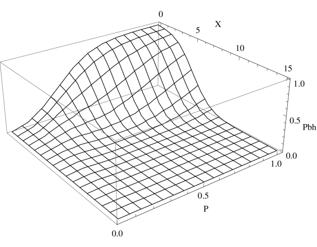
Figure 3: Probability the two-particle system is a BH as a function of $X$ and $P$ (in units of Planck length and mass respectively).

One then finds that $P_{\rm H}=|\psi_{\rm H}(R_{\rm H})|^{2}$ shows a mild dependence on $X$ (see Fig. 1) and a strong dependence on $P$ (see Fig. 2), in agreement with the fact that the energy of the system only depends on $P$, and not on the spatial separation between the two particles. It is also worth noting that $P_{\rm H}(R_{\rm H})$ always peaks around $R_{\rm H}\simeq 2\,\ell_{\rm p}\,(2P/m_{\rm p})$, in very good agreement with the hoop conjecture (1).

The probability (10) that the system of two particles is a BH can next be computed numerically as a function of the distance from the centre of mass $X$ of each particle, and the total energy $2P$. Fig. 3 shows the result for a suitable range of $X$ and $P$. Note that a first estimate of what happens as the two particles evolve in time can be obtained by considering the probability $P_{\rm BH}=P_{\rm BH}(X,2P)$ along lines of constant $P$ and decreasing $X$: $P_{\rm BH}$ clearly increases up to the maximum reached for $X=0$, when the two (non-interacting) particles exactly superpose. There is therefore a significant probability that the collision produces a BH, say $P_{\rm BH}(X,2P\gtrsim 2m_{\rm p})\gtrsim 80\%$, if the distance from the centre of mass and linear momentum  satisfy

$$X\lesssim{2\,\ell_{\rm p}}\,\frac{2P}{m_{\rm p}}-{\ell_{\rm p}}=R_{\rm H}(2P)-\ell_{\rm p}\ ,$$ (22)

where the term $-\ell_{\rm p}$ on the right is the “QM correction” to the hoop formula (1) for $E\simeq 2P\gtrsim 2\,m_{\rm p}$, which applies to the formation of large (semi)classical BHs. For lower values of $P$, $P_{\rm BH}(X,2P\lesssim 2m_{\rm p})\gtrsim 80\%$ for $2P\gtrsim m_{\rm p}\,(1+X^{2}/9\,\ell_{\rm p}^{2})$ and the limiting curve $P_{\rm BH}(X,2P\lesssim 2m_{\rm p})\simeq 80\%$ can be approximated by

$$2P-m_{\rm p}\simeq m_{\rm p}\,\frac{X^{2}}{9\,\ell_{\rm p}^{2}}\ ,$$ (23)

which crosses the axis $X=0$ for $2P\simeq m_{\rm p}$ [instead of $2P\simeq m_{\rm p}/2$, as it would follow from the linear relation (22)]. Eq. (23) represents a QM correction to the hoop conjecture (1) for quantum BH production. Let us note that, of course, different numerical coefficients are obtained if one takes other values of $P_{\rm BH}$ as a reasonably large probability, but the slope in Eq. (22) remains stably in agreement with Eq. (1).

IV Conclusions and outlook

Based upon the analytical results (22) and (23), we argue that the hoop conjecture can be extended into the QM description of BH formation, with a consistent probabilistic interpretation carried by the horizon wave-function of the given system. It is nonetheless important to remark again that this rather neat conclusion stems from several strong approximations.

First of all, we have totally neglected any sort of interaction between the particles, including gravitational tidal forces (which are very likely to play some part at the Planck scale, and which will be investigated in the future). In this respect, let us note that the flat space dispersion relation (14) might be appropriate for describing a single spherically symmetric particle, since the relevant energy that determines its Schwarzschild radius (1) is actually the Misner-Sharp mass $M$ defined in Eq. (4) by means of the flat space volume measure. Other spherically symmetric systems, such as concentric shells and spheres of matter, are presently being analysed within this formalism. However, once the spherical symmetry is broken, like it is for a system of two or more colliding particles in more than one spatial dimension, the effect on the space-time induced by each particle should be accounted for. A way to address this issue is, for example, to employ suitably modified dispersion relations, tantamount to a modified spectral decomposition in Eq. (6).

Moreover, we just considered a one-dimensional space also in order to avoid the kinematical complication of non-vanishing impact parameter and angular momentum of the system of two particles. However, it is worth recalling the original hoop conjecture should apply to trapping surfaces, and the formation of the latter in a non-spherical massive system has been thoroughly investigated in Ref. malec . The extension of the present analysis to collisions in three spatial dimensions is currently being investigated and we can foresee significant technical complications. In fact, Eq. (1) and the spectral decomposition of matter states must be replaced by the corresponding expressions for a rotating BH, but the approach still looks promising.

Let us then conclude by mentioning a further issue that has not yet been addressed: we are all aware that, in very high energy collisions, quantum states cannot be simply viewed as representing a fixed number of particles. Indeed, the historical motivation for QFT was to account for particle production and annihilation in such processes, which has made the very concept of “localisation” problematic. Since, conversely, the very concept of horizon is related to the localisation of the matter source, one can expect that implementing the formalism of the horizon wave-function in full-fledged QFT might lead to some surprises.

References

- (1) J.R. Oppenheimer and H. Snyder, Phys. Rev. 56, 455 (1939); J.R. Oppenheimer and G.M. Volkoff, Phys. Rev. 55, 374 (1939).
- (2) P.S. Joshi, “Gravitational Collapse and Spacetime Singularities,” Cambridge Monographs on Mathematical Physics (Cambridge, 2007).
- (3) K.S. Thorne, “Nonspherical Gravitational Collapse: A Short Review,” in J.R. Klauder, Magic Without Magic, San Francisco (1972), 231.
- (4) P.D. D’Eath and P.N. Payne, Phys. Rev. D 46, 658 (1992); Phys. Rev. D 46, 675 (1992); Phys. Rev. D 46, 694 (1992).
- (5) N.O. Murchadha, R.-S. Tung, N. Xie and E. Malec, Phys. Rev. Lett. 104, 041101 (2010); P. Bizon, E. Malec and N. O’Murchadha, Phys. Rev. Lett. 61, 1147 (1988).
- (6) T. Banks and W. Fischler, “A Model for high-energy scattering in quantum gravity,” hep-th/9906038; D.M. Eardley and S.B. Giddings, Phys. Rev. D 66, 044011 (2002); S.B. Giddings and S.D. Thomas, Phys. Rev. D 65, 056010 (2002).
- (7) G.L. Alberghi, R. Casadio, O. Micu and A. Orlandi, JHEP 1109, 023 (2011).
- (8) R. Casadio, “Localised particles and fuzzy horizons: A tool for probing Quantum Black Holes,” arXiv:1305.3195 [gr-qc]; R. Casadio and F. Scardigli, Eur. Phys. J. C 74, 2685 (2014).
- (9) S.D.H. Hsu, Phys. Lett. B 555, 92 (2003). X. Calmet, D. Fragkakis and N. Gausmann, Eur. Phys. J. C 71, 1781 (2011); X. Calmet, W. Gong and S.D.H. Hsu, Phys. Lett. B 668, 20 (2008).
- (10) G. Dvali and C. Gomez, Eur. Phys. J. C 74, 2752 (2014); Phys. Lett. B 719, 419 (2013); Phys. Lett. B 716, 240 (2012); Fortsch. Phys. 61, 742 (2013); R. Casadio and A. Orlandi, JHEP 1308, 025 (2013).
- (11) S. Doplicher, G. Morsella and N. Pinamonti, J. Geom. Phys. 74, 196 (2013).
- (12) E. Malec, Phys. Rev. Lett. 67, 949 (1991).