Sensing and Recognition When Primary User Has Multiple Power Levels

Abstract

In this paper, we present a new cognitive radio (CR) scenario when the primary user (PU) operates under more than one transmit power levels. Different from the existing studies where PU is assumed to have only one constant transmit power, the new consideration well matches the practical standards, i.e., IEEE 802.11 Series, GSM, LTE, LTE-A, etc., as well as the adaptive power concept that has been studied over the past decades. The primary target in this new CR scenario is, of course, still to detect the presence of PU. However, there appears a secondary target as to identify the PU’s transmit power level. Compared to the existing works where the secondary user (SU) only senses the “on-off” status of PU, recognizing the power level of PU achieves more “cognition”, and could be utilized to protect different powered PU with different interference levels. We derived quite many closed-form results for either the threshold expressions or the performance analysis, from which many interesting points and discussions are raised. We then further study the cooperative sensing strategy in this new cognitive scenario and show its significant difference from traditional algorithms. Numerical examples are provided to corroborate the proposed studies.

I Introduction

Cognitive radio (CR) has been recognized as a promising solution to spectrum scarcity and spectrum under-utilization [1] by allowing the secondary users (SUs) to access the spectrum of the primary user (PU) when the latter is idle. The key component of CR is thus the spectrum sensing that could detect whether a specific frequency band is being used by PU or not.

Popular spectrum sensing techniques that have been proposed include matched filter detection [2], energy detection [3, 4, 5], and cyclostationary detection [6, 7], among which energy detection has received intensive attention because it requires the least prior knowledge of PU and is very simple to implement. The only prerequisite of the energy detection is that SU knows noiseless receive power (possibly need to know the transmit power of PU and path statistics from PU to SU or their product), and then one can derive a threshold $\lambda$ such that the truly received energy being greater than $\lambda$ tells the presence of PU or otherwise tells the absence of PU. When SU is equipped with multiple antennas, a promising sensing technology was designed in [8] where the eigenvalues of the receive covariance matrix are used to judge the status of PU. It is shown that the performance of multiple antenna based spectrum sensing is much better than that from a single antenna [9] because the former fully utilizes the correlation among antennas. On the other side, when multiple antenna is infeasible due to the size limitation of the wireless terminal, one can refer to the cooperative spectrum sensing from more than one SUs to enhance the sensing performance [10, 11, 12].

There are also quite a number of works related to CR over the past ten years. For example, parameter uncertainty based spectrum sensing [13], design with imperfect sensing [14], sensing throughput tradeoff [15], sensing based sharing [16], spectrum sharing [17], as well as many other hybrid schemes between CR and other technologies, e.g., games among SUs [18], sensing in OFDM system [19], sensing in relay network [20], and many others. We may confidently claim that CR has opened a new research field in wireless communications and has achieved fruitful research results.

However, it is not difficult to notice that all the existing spectrum sensing techniques [2]–​​[12] as well as the related studies [13]–​​[20] assume PU either be absent or be present with a constant power. Yet, it can be easily known from the current standards, i.e., IEEE 802.11 series [21], GSM [22], and the future standards, i.e., LTE [23], LTE-A [24] that the licensed users could be working under different transmit power levels in order to cope with different situations, e.g., environment, rate, etc. A typical example is in CDMA [25] uplink scenario when the users are subjected to the power control to cope with the near-far effects. In fact, varying transmit power of the licensed user is a natural functionality and should be taken into consideration as witnessed by so many existing literatures studying the power allocation problem [26, 27]. Therefore, the traditional spectrum sensing techniques, which only considers a constant power level of PU, is not adequate to match both the practical situations and the theoretical demands.

In fact, FCC [31] has specified the interference protection requirements for TV white space, and the requirements for different powered services, e.g., full-power digital TV, full-power analog TV, low-power analog TV, low-power digital TV, etc., are different as shown in Table I. It is then clear that by detecting the power levels of PU, SU could adjust its transmit power to meet the interference requirement for different powered PU. Therefore, the sensing target when PU has multiple power levels should not only be detecting the on-off status of PU but also to identify its power level. To the best of the authors’ knowledge, the only work that considers this multiple power transmit power (MPTP) scenario is [29], where the authors briefly present the new sensing strategy while focus more on the optimal power allocation of SU after power-level recognition in order to maximize secondary throughput. Unfortunately, [29] does not fully discuss the fundamentals issues of spectrum sensing in MPTP and possesses many careless results.

In this paper, we provide a thorough investigation over the spectrum sensing in MPTP scenario and design two different sensing strategies. We derive closed form expressions of decision regions and discussed the power-mask effect, which is shown to be an unique phenomenon in MPTP scenario. We also provide many remarks explaining the fundamental reasoning behind the multiple hypothesis detection in MPTP based CR. To improve the sensing performance, we further propose two cooperative sensing schemes, which show much difference from the traditional cooperative sensing. The closed-form performance analysis of all four sensing algorithms are derived too. Various numerical examples are provided to corroborate the proposed studies.

The rest of the paper is organized as follows. Section II presents the system model of MPTP scenario. In Section III, we propose two different spectrum sensing strategies and discuss their relationship. In Section IV, we investigate cooperative sensing in MPTP scenario and derive two different algorithms based on the majority voting and the MAP detection, respectively. In Section V, simulations results are provided to evaluate the designed algorithms. Finally, conclusions are drawn in Section VI.

II System Model

Consider a simple CR network that consists of one PU, $K$ SUs and a common receiver, i.e., the decision fusion center. The primary user (PU) could either be absent or operate under one power-level $P_{i},i\in\{1,2,\ldots,N\}$. Without loss of generality, we assume $P_{i+1}>P_{i}>0,\forall i$. As one of the earliest work considering the MPTP scenario, we assume the values of the noiseless received powers $\gamma_{k}P_{i},\ \forall i$, are known at SU-$k$. More considerable situations, e.g., partially known channels or power levels could serve as future research topics.

During the sensing time, the $l$th received sample at SU-$k$ can be expressed as:

$$x_{l,k}=\left\{\begin{array}[]{ll}n_{l,k}&{\cal H}_{0}\\ \sqrt{P_{i}}\sqrt{\gamma_{k}}s_{l,k}+n_{l,k}&{\cal H}_{i},\ i=1,2,...,N\end{array}\right.$$ (3)

where ${\cal H}_{0}$ denotes the hypothesis that PU is absent while ${\cal H}_{i}$ indicates PU is operating under power-level $P_{i}$; $s_{l,k}$ is the $l$th sample transmitted from PU, which is assumed to follow complex Gaussian distribution with zero mean and unit variance, i.e., $s_{l,k}\sim{\cal CN}(0,1)$; $n_{l}$ is the additive noise that follows ${\cal CN}(0,\sigma^{2}_{n})$ for all cases. If we define $P_{0}=0$ as the power when PU is absence, then a unified expression can be obtained as

$$x_{l,k}\sim{\cal CN}(0,\gamma_{k}P_{i}+\sigma^{2}_{n}),\quad\forall{\cal H}_{i},\ i\in\{0,1,\ldots,N\},$$ (4)

Let us define the prior probability of each state of PU as $\text{Pr}({\cal H}_{i}),\ i=0,1,\ldots,N$. Then, the presence state of PU will include all ${\cal H}_{i},i\geq 1$ and will be denoted as ${\cal H}_{\text{on}}$. Obviously, ${\cal H}_{\text{on}}$ has the prior probability $\text{Pr}({\cal H}_{\text{on}})=\sum_{i=1}^{N}\text{Pr}({\cal H}_{i})$, while the absence state of PU, denoted by ${\cal H}_{\text{off}}\triangleq{\cal H}_{0}$, has the probability $\text{Pr}({\cal H}_{\text{off}})=\text{Pr}({\cal H}_{0})$.

In MPTP scenario, we define the primary target of spectrum sensing as detecting the presence of PU, while define the secondary target as recognizing the power-level of PU. As mentioned in Section I, PU may operate in different power levels, each with a different tolerable interference level from SU. After recognizing the power level of PU, SU could choose a proper transmit power to fulfill the interference requirements.

III Spectrum Sensing at Local SU

Let us first present how local secondary user (e.g., SU-$k$) performs spectrum sensing in MPTP scenario. The user index $k$ is thus dropped for notation conciseness. We propose the following two different but relevant approaches.

III-A Sensing Strategy-I: Detecting the Presence First

Since we define the primary task in MPTP as to check the presence of PU, we may first verify the hypothesis ${\cal H}_{\text{on}}/{\cal H}_{\text{off}}$. If ${\cal H}_{\text{on}}$ is detected, then the next step is to recognize which ${\cal H}_{i},i\geq 1$ is true. Let us assume that SU receives a total number of $M$ samples during the sensing period, denoted as $\mathbf{x}=[x_{1},x_{2},\ldots,x_{M}]^{T}$. The ratio of the posterior probabilities between two hypothesis can be written as

$$\eta(\mathbf{x})= \frac{\text{Pr}({\cal H}_{\text{on}}|\mathbf{x})}{\text{Pr}({\cal H}_{\text{off}}|\mathbf{x})}=\frac{\sum_{i=1}^{N}\text{Pr}({\cal H}_{i}|\mathbf{x})}{\text{Pr}({\cal H}_{0}|\mathbf{x})}=\sum_{i=1}^{N}\frac{p(\mathbf{x}|{\cal H}_{i})\text{Pr}({\cal H}_{i})}{p(\mathbf{x}|{\cal H}_{0})\text{Pr}({\cal H}_{0})}$$

$$= \sum_{i=1}^{N}\frac{\text{Pr}({\cal H}_{i})}{\text{Pr}({\cal H}_{\text{off}})}\bigg{(}\frac{\sigma^{2}_{n}}{\gamma P_{i}+\sigma^{2}_{n}}\bigg{)}^{M}\text{exp}\bigg{\{}\frac{\gamma P_{i}\sum_{l=1}^{M}|x_{l}|^{2}}{\sigma^{2}_{n}(\gamma P_{i}+\sigma^{2}_{n})}\bigg{\}}.$$ (5)

It is easily seen that $\eta(\mathbf{x})$ is strictly increasing over $y\triangleq\sum_{l=1}^{M}|x_{l}|^{2}$, i.e., the received energy, so the decision can be alternatively made through

$$y\mathop{\gtrless}\limits_{\mathcal{H}_{\text{off}}}^{\mathcal{H}_{\text{on}}}\theta,$$ (6)

where $\theta$ is the pre-determined parameter. Hence, the optimal detector is the energy detector and we can re-represent $\eta(\mathbf{x})$ as $\eta(y)$ . The parameter $\theta$ is used to control the detection performance. For example if $\theta$ is used to control the false alarm probability, then the detection follows Neyman Pearson rule; If $\theta$ is set such that $\eta(y)=1$, then the detection follows the maximum a posterior (MAP) rule .

The probability density functions (pdf) of $y$ conditioned on $\mathcal{H}_{i},\ i\in\{0,1,\ldots,N\}$ and $\mathcal{H}_{\text{on}}$ can be derived as

$$p(y|{\cal H}_{i})=\frac{y^{M-1}e^{-\frac{y}{\gamma P_{i}+\sigma^{2}_{n}}}}{\Gamma(M)(\gamma P_{i}+\sigma^{2}_{n})^{M}},$$ (7)

$$p(y|{\cal H}_{\text{on}})=\sum_{i=1}^{N}p(y|{\cal H}_{i})\frac{\text{Pr}{({\cal H}_{i})}}{\text{Pr}({\cal H}_{\text{on}})}=\frac{1}{\text{Pr}({\cal H}_{\text{on}})}\sum_{i=1}^{N}p(y|{\cal H}_{i})\text{Pr}{({\cal H}_{i})},$$ (8)

where $\Gamma(\cdot)$ denotes the gamma function.

Similar to the conventional CR, we could resort to the false alarm probability and the detection probability to describe the performance of the detection, separately calculated as

$$\text{P}_{\text{fa}}(\theta) =\text{Pr}(\mathcal{H}_{\text{on}}|\mathcal{H}_{\text{off}})=\int_{\theta}^{\infty}p(y|\mathcal{H}_{\text{off}})dy=\frac{\gamma(M,\frac{\theta}{\sigma^{2}_{n}})}{\Gamma(M)},$$ (9)

$$\text{P}_{\text{d}}(\theta) =\text{Pr}(\mathcal{H}_{\text{on}}|\mathcal{H}_{\text{on}})=\frac{1}{\text{Pr}(\mathcal{H}_{\text{on}})}\sum_{i=1}^{N}\int_{\theta}^{\infty}\!\!p(y|\mathcal{H}_{i})\text{Pr}(\mathcal{H}_{i})dy=\sum_{i=1}^{N}\!\!\frac{\gamma(M,\frac{\theta}{\gamma P_{i}+\sigma^{2}_{n}})}{\Gamma(M)}\frac{\text{Pr}(\mathcal{H}_{i})}{\text{Pr}(\mathcal{H}_{\text{on}})},$$ (10)

where $\gamma(\cdot,\cdot)$ denotes the lower incomplete gamma function and $\theta$. As usual, one can adjust $\theta$ to achieve a desired $\text{P}_{\text{fa}}(\theta)$, and then the corresponding $\text{P}_{\text{d}}(\theta)$ is immediately settled.

Let us compute the threshold $\theta_{\text{on/off}}$ according to MAP criterion for consistency in the rest of the paper. From (III-A), $\theta_{\text{on/off}}$ could be obtained from $\eta(\theta_{\text{on/off}})=1$ and can be numerically computed from the equation $\Phi(\theta)=0$, where $\Phi(\theta)$ is defined as

$$\Phi(\theta)\triangleq\sum_{i=1}^{N}\frac{\text{Pr}({\cal H}_{i})}{(\frac{\gamma_{k}P_{i}}{\sigma^{2}_{n}}+1)^{M}}\text{\large e}^{\frac{\gamma_{k}P_{i}}{\sigma^{2}_{n}(\gamma_{k}P_{i}+\sigma^{2}_{n})}\cdot\theta}-\text{Pr}({\cal H}_{0}).$$ (11)

It can be easily checked that $\frac{\partial\Phi(\theta)}{\partial\theta}>0$ and $\Phi(0)<0$ as long as $M$ is sufficiently large. Hence the solution $\theta_{\text{on/off}}$ that makes $\Phi(\theta)=0$ must exist and is definitely unique as well.

If the received energy satisfy $y>\theta_{\text{on/off}}$, then PU is claimed to be present and the next step is to recognize which power-level of PU is in use. A natural approach is to formulate multiple hypothesis testing [30] and apply MAP detection, where for a hypothesis pair $({\cal H}_{i},{\cal H}_{j})$, $\forall i,j\geq 1$, ${\cal H}_{i}$ beats ${\cal H}_{j}$ if

$$\text{Pr}({\cal H}_{i}|\mathbf{x},\hat{{\cal H}}_{\text{on}})>\text{Pr}({\cal H}_{j}|\mathbf{x},\hat{{\cal H}}_{\text{on}}).$$ (12)

Here, we use $\hat{{\cal H}}_{\text{on}}$ to denote that the presence detection has been made already. From Bayes rule, there is

$$\text{Pr}({\cal H}_{i}|\mathbf{x},\hat{{\cal H}}_{\text{on}})= \frac{p(\mathbf{x}|{\cal H}_{i},\hat{{\cal H}}_{\text{on}})\text{Pr}({\cal H}_{i}|\hat{{\cal H}}_{\text{on}})}{p(\mathbf{x}|\hat{{\cal H}}_{\text{on}})}.$$ (13)

Let us define the equivalent region of $\mathbf{x}\in{\cal X}$ to $y>\theta_{\text{on/off}}$, and then represent $\hat{{\cal H}}_{\text{on}}$ as $\mathbf{x}\in{\cal X}$. Then (13) can be rewritten as

$$\text{Pr}({\cal H}_{i}|\mathbf{x},\hat{{\cal H}}_{\text{on}})= \frac{1}{p(\mathbf{x}|\mathbf{x}\in{\cal X})}\cdot p(\mathbf{x}|{\cal H}_{i},\mathbf{x}\in{\cal X})\cdot\text{Pr}({\cal H}_{i}|\mathbf{x}\in{\cal X})$$

$$= \frac{1}{p(\mathbf{x}|\mathbf{x}\in{\cal X})}\cdot\frac{p(\mathbf{x}|{\cal H}_{i})}{\text{Pr}(\mathbf{x}\in{\cal X}|{\cal H}_{i})}\cdot\frac{\text{Pr}(\mathbf{x}\in{\cal X}|{\cal H}_{i})\text{Pr}({\cal H}_{i})}{\text{Pr}(\mathbf{x}\in{\cal X})}$$

$$= \frac{p(\mathbf{x}|{\cal H}_{i})\text{Pr}({\cal H}_{i})}{p(\mathbf{x}|\mathbf{x}\in{\cal X})\text{Pr}(\mathbf{x}\in{\cal X})}.$$ (14)

Note that the following equality holds from the definition of probability density function

$$p(\mathbf{x}|{\cal H}_{i},\mathbf{x}\in{\cal X})=\frac{p(\mathbf{x}|{\cal H}_{i})}{\text{Pr}(\mathbf{x}\in{\cal X}|{\cal H}_{i})},\quad\mathbf{x}\in{\cal X}$$ (15)

and is used to derive (14). We place $\mathbf{x}\in{\cal X}$ in (15) to represents that (15) holds only for domain $\mathbf{x}\in{\cal X}$.

Therefore, the MAP detection (12) is simplified to

$$p(\mathbf{x}|{\cal H}_{i})\text{Pr}({\cal H}_{i})>p(\mathbf{x}|{\cal H}_{j})\text{Pr}({\cal H}_{j}),\quad\mathbf{x}\in{\cal X}$$ (16)

Remark 1

From (16), we know the MAP detection for power levels is not related with how ${\cal H}_{\text{on}}$ is detected, i.e., we can apply either MAP detection or Neyman Pearon to check the presence of PU without affecting (16). Nevertheless, the way to detect the presence of PU will affect the value of $\text{Pr}({\cal H}_{i}|\mathbf{x},\hat{{\cal H}}_{\text{on}})$ as seen from (14).

Hence, the MAP detection of the power level can be simply described as

$$\hat{i}=\arg\max_{i\in\{1,\ldots,N\}}\ p(\mathbf{x}|{\cal H}_{i})\text{Pr}({\cal H}_{i}),\quad\mathbf{x}\in{\cal X}.$$ (17)

Let us then define the ratio

$$\xi(\mathbf{x})=\frac{p(\mathbf{x}|{\cal H}_{i})\text{Pr}({\cal H}_{i})}{p(\mathbf{x}|{\cal H}_{j})\text{Pr}({\cal H}_{j})}=\frac{\text{Pr}(\mathcal{H}_{i})}{\text{Pr}(\mathcal{H}_{j})}\bigg{(}\frac{\gamma P_{j}+\sigma^{2}_{n}}{\gamma P_{i}+\sigma^{2}_{n}}\bigg{)}^{M}\text{exp}\bigg{\{}\frac{\gamma(P_{i}-P_{j})\sum_{l=1}^{M}|x_{l}|^{2}}{(\gamma P_{i}+\sigma^{2}_{n})(\gamma P_{j}+\sigma^{2}_{n})}\bigg{\}}.$$ (18)

Obviously, $\xi(\mathbf{x})$ is purely related with the energy $y=\sum_{l=1}^{M}|x_{l}|^{2}$ (other variables are constants). Hence, the energy detector is again optimal when recognizing the power level of PU, and we can represent $\xi(\mathbf{x})$ by $\xi(y)$. Since $\xi(\mathbf{x})$ is an increasing function of $y$ when $P_{i}>P_{j}$, one can easily know that the decision region of ${\cal H}_{i}$, denoted as ${\cal R}(\mathcal{H}_{i})$, must be a continuous region of $y$, and ${\cal R}(\mathcal{H}_{i})$ must stay on the right side of ${\cal R}(\mathcal{H}_{j})$ if $P_{i}>P_{j}$.

Theorem 1

The decision regions of hypothesis $\mathcal{H}_{i},\ i\in\{1,2,\ldots,N\}$ are

$${\cal R}(\mathcal{H}_{i}):=\left\{\begin{array}[]{ll}y\in\big{(}\theta_{\text{on/off}},\ \min_{1<j\leq N}\Theta(1,j)\big{)}&i=1\\ y\in\big{(}\max\{\theta_{\text{on/off}},\max_{1\leq j<i}\Theta(i,j)\},\ \min_{i<j\leq N}\Theta(i,j)\big{)},&1<i<N\\ y\in\big{(}\max\{\theta_{\text{on/off}},\max_{1\leq j<N}\Theta(N,j)\},\ +\infty\Big{)},&i=N\end{array}\right.$$ (22)

where $\Theta(i,j)$ is defined as

$$\Theta(i,j)\triangleq\frac{(\gamma P_{i}+\sigma^{2}_{n})(\gamma P_{j}+\sigma^{2}_{n})}{\gamma(P_{i}-P_{j})}\ln\bigg{[}\bigg{(}\frac{\gamma P_{i}+\sigma^{2}_{n}}{\gamma P_{j}+\sigma^{2}_{n}}\bigg{)}^{M}\frac{\text{Pr}({\cal H}_{j})}{\text{Pr}({\cal H}_{i})}\bigg{]}.$$ (23)

Proof:

Substituting (18) into (16) yields

$$\frac{y\cdot\gamma(P_{i}-P_{j})}{(\gamma P_{i}+\sigma^{2}_{n})(\gamma P_{j}+\sigma^{2}_{n})}>\ln\bigg{[}\bigg{(}\frac{\gamma P_{i}+\sigma^{2}_{n}}{\gamma P_{j}+\sigma^{2}_{n}}\bigg{)}^{M}\frac{\text{Pr}({\cal H}_{j})}{\text{Pr}({\cal H}_{i})}\bigg{]},\quad\forall i,j\geq 1.$$

If $P_{i}>P_{j}$, i.e., $i>j$, then there is

$$y>\frac{(\gamma P_{i}+\sigma^{2}_{n})(\gamma P_{j}+\sigma^{2}_{n})}{\gamma(P_{i}-P_{j})}\ln\bigg{[}\bigg{(}\frac{\gamma P_{i}+\sigma^{2}_{n}}{\gamma P_{j}+\sigma^{2}_{n}}\bigg{)}^{M}\frac{\text{Pr}({\cal H}_{j})}{\text{Pr}({\cal H}_{i})}\bigg{]},\quad\forall i>j;$$

If $P_{i}<P_{j}$, i.e., $i<j$, then there is

$$y<\frac{(\gamma P_{i}+\sigma^{2}_{n})(\gamma P_{j}+\sigma^{2}_{n})}{\gamma(P_{i}-P_{j})}\ln\bigg{[}\bigg{(}\frac{\gamma P_{i}+\sigma^{2}_{n}}{\gamma P_{j}+\sigma^{2}_{n}}\bigg{)}^{M}\frac{\text{Pr}({\cal H}_{j})}{\text{Pr}({\cal H}_{i})}\bigg{]},\quad\forall i<j.$$

Then for $1<i<N$, the lower bound of ${\cal R}(\mathcal{H}_{i})$ should be $y>\max\limits_{1\leq j<i}\Theta(i,j)$ and the upper bound should be $y<\min\limits_{i<j\leq N}\Theta(i,j)$. Moreover, the MAP detection is defined on the domain $\mathbf{x}\in{\cal X}$, i.e., $y>\theta_{\text{on/off}}$, so all decision regions of non-zero power should stay in $(\theta_{\text{on/off}},+\infty)$. Bearing in mind that $\theta_{\text{on/off}}$ may be greater than $\max\limits_{1\leq j<i}\Theta(i,j)$ for some $i$, the proof is completed. ∎

Remark 2

The decision region of ${\cal H}_{0}$, i.e., the absence of PU can be expressed in a unified way as

$${\cal R}(\mathcal{H}_{0}):=y\in\big{(}0,\ \theta_{\text{on/off}}\big{)}.$$ (24)

Remark 3

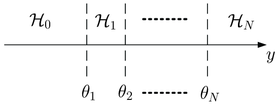
Figure 1: Multiple power level detections from multiple thresholds.

Compared to the traditional “on-off” based sensing that has only one threshold, the new scenario MPTP needs multiple thresholds to separate different power levels, as shown in Fig. 1, where $\theta_{1}\triangleq\theta_{\text{on/off}}$ is defined for consistence.

An interesting and special phenomenon in MPTP happens when the computed lower bound of a specific region ${\cal R}(\mathcal{H}_{i_{0}})$ is greater than the upper bound, e.g.,

$$\max\{\theta_{\text{on/off}},\ \max_{1\leq j<i_{0}}\Theta(i_{0},j)\}>\min_{i_{0}<j\leq N}\Theta(i_{0},j)$$ (25)

holds for some specific $1<i_{0}<N$. Once this happens then ${\cal R}(\mathcal{H}_{i_{0}})$ is empty and the power level $P_{i_{0}}$ can never be detected. We call this new phenomenon in MPTP as power-mask effect. Hence, in Fig. 1., the number of the thresholds may be less than or equal to $N$.

Remark 4

If $\theta_{\text{on/off}}>\max_{1\leq j<i_{0}}\Theta(i_{0},j)>\min_{i_{0}<j\leq N}\Theta(i_{0},j)$, then $P_{i_{0}}$ is masked from left by $P_{0}$, while if $\max_{1\leq j<i_{0}}\Theta(i_{0},j)>\theta_{\text{on/off}}>\min_{i_{0}<j\leq N}\Theta(i_{0},j)$, then $P_{i_{0}}$ is masked from both sides by $P_{i_{0}-1}$ and $P_{i_{0}+1}$.

Some intuitive explanation for power mask is provided here. First note that the bounds in the decision region ${\cal R}(\mathcal{H}_{i})$ are affected by many parameters, i.e., $P_{i}$, $\gamma$, $\sigma_{n}^{2}$, $\text{Pr}({\cal H}_{i})$. If the prior probability $\text{Pr}({\cal H}_{i_{0}})$ is very small, i.e., the power level $P_{i_{0}}$ is seldom used by PU. Then $P_{i_{0}}$ may easily be “ignored” by SU and is then masked. Another example is that, if $P_{i_{0}}$ is closed to $P_{i_{0}-1}$ and $P_{i_{0}+1}$ and if $\sigma_{n}^{2}$ is larger, then it is very possible that $P_{i_{0}}$ will be masked by $P_{i_{0}-1}$ or $P_{i_{0}+1}$ due to the large uncertainty caused by the noise.

Remark 5

Note that the leftmost level $P_{0}$ and the rightmost level $P_{N}$ cannot be masked and are always detectable.

Remark 6

When power-mask happens for a specific $i_{0}$, it means that the $P({\cal H}_{i_{0}}|\mathbf{x})$ cannot beat any other $P({\cal H}_{i}|\mathbf{x}),i\neq i_{0}$ but $P({\cal H}_{i_{0}}|\mathbf{x})$ could still possess non-zero value. Hence, it is possible to design some sophisticated approach which considers this “soft” information and remove the power-mask effect. Nevertheless, the corresponding discussion is out of the scope of this paper and will be left for future research.

Remark 7

It is of interest to check whether the decision regions for ${\cal H}_{i}$’s are continuously connected for two consecutively detectable indices $1<i_{0}<i_{0}+1<N$, i.e., for those not masked power level, check whether $\min_{i_{0}<j\leq N}\Theta(i_{0},j)=\max_{1\leq j<i_{0}+1}\Theta(i_{0}+1,j)$ holds. Unfortunately, due to the discrete nature of the power mask effect, we cannot mathematically prove this property. Nevertheless, it can be easily known that, for any $y$, there is always a corresponding decision according to the MAP detection (17). Therefore, there should be no gap between any two consecutive decision regions.

A special case that affects the power-mask effect appears when $\text{Pr}(P_{i})=\text{Pr}(P_{j}),\ \forall i,j\in\{1,2,\ldots,N\}$.

Lemma 1

If $\text{Pr}(P_{i})=\text{Pr}(P_{j})$ holds for $\forall i,j\in\{1,2,\ldots,N\}$, then $\Theta(i,j)$ is not related to $P({\cal H}_{i})$ and is an increasing function over $P_{j}$ for any $P_{i}$.

Proof:

In this case, take the partial derivative of $\Theta(i,j)$ over $P_{j}$ as

$$\frac{\partial\Theta(i,j)}{\partial P_{j}} =\frac{M(\gamma P_{i}+\sigma^{2}_{n})^{2}}{\gamma(P_{j}-P_{i})^{2}}\bigg{\{}\frac{\gamma(P_{j}-P_{i})}{\gamma P_{i}+\sigma^{2}_{n}}-\ln\Big{[}1+\frac{\gamma(P_{j}-P_{i})}{\gamma P_{i}+\sigma^{2}_{n}}\Big{]}\bigg{\}}.$$ (26)

Redefining $z=\frac{\gamma(P_{j}-P_{i})}{\gamma P_{i}+\sigma^{2}_{n}}$, it can be easily known that $z\in(-1,+\infty)$ for any $i$. We then obtain

$$\frac{\partial\Theta(i,j)}{\partial P_{j}}=\frac{M\gamma}{z^{2}}\big{[}z-\ln(1+z)\big{]}.$$

It is also clear that $z-\ln(1+z)\geq 0$ for $z>-1$. Hence, $\frac{\partial\Theta(i,j)}{\partial P_{j}}\geq 0$ holds for all possible $P_{j}$ and $\Theta(i,j)$ is an increasing function over $P_{j}$. ∎

According to Lemma 1, when $\text{Pr}(P_{i})=\text{Pr}(P_{j}),i,j\geq 1$ there is

$$\max_{1\leq j<i}\Theta(i,j)=\Theta(i,i-1)<\Theta(i,i+1)=\min_{i<j\leq N}\Theta(i,j).$$ (27)

Therefore, the non-zero power levels cannot mask each other, while the power mask effect may only happen when $P_{0}$ mask the power levels on its right side.

Remark 8

When $\text{Pr}(P_{i})=\text{Pr}(P_{j}),i,j\geq 1$, denote the first power level that is not masked by $P_{0}$ as $P_{i_{0}}$. It can be readily check that all the power levels on its right sides, i.e., $P_{i},i>i_{0}$ has $\Theta(i,i+1)=\Theta(i+1,i)$, and hence the decision regions for all ${\cal H}_{i}$’s are mathematically proved to be connected in this case.

Note that the decision range ${\cal R}(\mathcal{H}_{i})$ can be determined in a prior manner by calculating all $\Theta(i,j)$ and $\theta_{\text{on/off}}$ in advance. To unify our discussion, let us use $\theta_{i},i\in\{1,2,\ldots,N\}$ to denote the threshold between ${\cal R}(\mathcal{H}_{i-1})$ and ${\cal R}(\mathcal{H}_{i})$, and define $\theta_{0}\triangleq 0$, $\theta_{N+1}\triangleq+\infty$ for completeness. Meanwhile, if $P_{i_{0}}$ cannot be detected due to power-mask effect, we denote $\theta_{i_{0}}=\theta_{i0+1}$ so that the corresponding decision range $[\theta_{i_{0}},\theta_{i_{0}+1})$ is empty.

To characterize the performance of the spectrum sensing in MPTP, purely resorting to $\text{P}_{\text{d}}(\theta)$ and $\text{P}_{\text{fa}}(\theta)$ is not adequate. We should calculate all the probabilities when SU makes the decision as hypothesis $\mathcal{H}_{j}$ while PU is actually transmitting with $P_{i}$, that is

$$\text{Pr}(\mathcal{H}_{j}|\mathcal{H}_{i})= \int_{\theta_{j}}^{\theta_{j+1}}p(y|\mathcal{H}_{i})dy=\frac{\gamma\left(M,\frac{\theta_{j}}{\gamma P_{i}+\sigma^{2}_{n}}\right)}{\Gamma(M)}-\frac{\gamma\left(M,\frac{\theta_{j+1}}{\gamma P_{i}+\sigma^{2}_{n}}\right)}{\Gamma(M)},\quad\forall i,j,$$ (28)

which is also defined as decision probability in this paper. Obviously, the decision probabilities of those masked power are zeros.

Then, $\text{P}_{\text{d}}(\theta)$ and $\text{P}_{\text{fa}}(\theta)$ can be easily obtained from the summations of the corresponding $\text{Pr}(\mathcal{H}_{j}|\mathcal{H}_{i})$. Moreover we may introduce a new technical term

$$P_{\text{dis1}}=\frac{1}{\text{Pr}(\cal H_{\text{on}})}\sum_{i=1}^{N}\text{Pr}({\cal H}_{i}|{\cal H}_{i})P({\cal H}_{i}),$$ (29)

named as discrimination probability to describe the recognition capability for our secondary target.

III-B Sensing Strategy II: Recognize Power Level First

Another reasonable approach to achieve both our targets is to directly detecting the power level of PU by treating $P_{0}$ as an equivalent power level (but with zero value) as other non-zero $P_{i},i\geq 1$. The presence or the absence can be immediately found after the power level index is detected.

From MAP based multiple hypothesis testing, the optimal detection can be stated as

$$\hat{i}=\arg\max_{i\in\{0,1,\ldots,N\}}\ \text{Pr}({\cal H}_{i}|\mathbf{x}).$$ (30)

Since the expression of (30) is, mathematically, the same as (17) but includes one more index $0$, the previous results can be immediately modified here. For example, the decision region is computed as

$${\cal R}(\mathcal{H}_{i}):=\left\{\begin{array}[]{ll}y\in\big{(}0,\ \min_{0<j\leq N}\Theta(0,j)\big{)}&i=0\\ y\in\big{(}\max_{0\leq j<i}\Theta(i,j),\ \min_{i<j\leq N}\Theta(i,j)\big{)},&0<i<N\\ y\in\big{(}\max_{0\leq j<N}\Theta(N,j),\ +\infty\Big{)},&i=N\end{array}\right.$$ (34)

where $\Theta(i,j)$ is given in (23). Hence, the power-mask effect also exists if $\max_{1\leq j<i_{0}}\Theta(i_{0},j)>\min_{i_{0}<j\leq N}\Theta(i_{0},j)$ for some $i_{0}$. Let us use $\phi_{i}$ to represent the thresholds separating ${\cal R}(\mathcal{H}_{i-1})$ and ${\cal R}(\mathcal{H}_{i})$. Then the decision probability is given in (28) with $\theta_{i}$ being replaced by $\phi_{i}$.

Remark 9

In sensing strategy-II, once again, both $P_{0}$ and $P_{N}$ cannot be masked and are always detectable.

Due to the similarity between the decision regions of the two sensing approaches, i.e., (22) and (34), one natural and interest question arises: are all the thresholds or parts of the thresholds the same in these two sensing approaches? Of all the thresholds, the first one $\theta_{\text{on/off}}$ that separates the absence decision and presence decision is of special importance. Then we provide the following lemma.

Lemma 2

Let $\phi_{\text{on/off}}\triangleq\phi_{1}$ be the threshold between detecting absence and detecting presence in sensing strategy II, there is $\phi_{\text{on/off}}>\theta_{\text{on/off}}$.

Proof:

Considering the power-mask effect, $\phi_{\text{on/off}}$ can be computed from $\text{Pr}({\cal H}_{0}|\mathbf{x})=\text{Pr}({\cal H}_{j_{0}}|\mathbf{x})$ where $j_{0}$ is the index of the first non-zero power that is not masked. From (18), we can derive a unique $\phi_{\text{on/off}}$ as

$$\phi_{\text{on/off}}=\frac{\sigma^{2}_{n}(\gamma P_{j_{0}}+\sigma^{2}_{n})}{\gamma P_{j_{0}}}\cdot\ln\bigg{[}\frac{\text{Pr}(\mathcal{H}_{0})}{\text{Pr}(\mathcal{H}_{j_{0}})}\Big{(}\frac{\gamma P_{j_{0}}}{\sigma^{2}_{n}}+1\Big{)}^{M}\bigg{]}.$$ (35)

Let us then compute $\Phi(\phi_{\text{on/off}})$ from (11), which yields

$$\Phi(\phi_{\text{on/off}}) =\sum_{i=1}^{N}\frac{\text{Pr}({\cal H}_{i})}{(\frac{\gamma P_{i}}{\sigma^{2}_{n}}+1)^{M}}\text{\large e}^{\frac{\gamma P_{i}}{\sigma^{2}_{n}(\gamma P_{i}+\sigma^{2}_{n})}\cdot\phi_{\text{on/off}}}-\text{Pr}({\cal H}_{0})$$

$$=\sum_{i\neq j_{0}}^{N}\frac{\text{Pr}({\cal H}_{i})}{(\frac{\gamma P_{i}}{\sigma^{2}_{n}}+1)^{M}}\text{\large e}^{\frac{\gamma P_{i}}{2\sigma^{2}_{n}(\gamma P_{i}+\sigma^{2}_{n})}\cdot\phi_{\text{on/off}}}>0.$$

Since $\Phi(\theta_{\text{on/off}})=0$ and $\Phi(\theta)$ is an increasing function over $\theta$, it is obvious that $\phi_{\text{on/off}}>\theta_{\text{on/off}}$. The lemma is proved. ∎

Lemma 2 suggests that sensing strategy-II claims more absence of PU than sensing strategy-I. In general, when we compare (34) and (22), it is easy to note that $\max_{0\leq j<i}\Theta(i,j)$ may be greater than $\max_{1\leq j<i}\Theta(i,j)$ if $\Theta(i,0)$ is the bigger than other $\Theta(i,j),\ 0<j<i$. When this happens, it also means that $P_{0}$ masks all power levels smaller than $P_{i+1}$ in sensing strategy-II. Hence, the lower bound of ${\cal R}(\mathcal{H}_{i})$ in sensing strategy-II is $\phi_{\text{on/off}}$ while the lower bound of ${\cal R}(\mathcal{H}_{i})$ in sensing strategy-I is $\max\{\theta_{\text{on/off}},\ \max_{1\leq j<i_{0}}\Theta(i_{0},j)\}$. Combing Lemma 2, it is then clear that the lower bound of ${\cal R}(\mathcal{H}_{i})$ in sensing strategy-II is bigger than that of sensing strategy-I. Nevertheless, when $\Theta(i,0)$ is not the dominant one in $\max_{0\leq j<i}\Theta(i,j)$, i.e., $\text{Pr}({\cal H}_{0}|\mathbf{x})$ is not the biggest among all $\text{Pr}({\cal H}_{i}|\mathbf{x})$, then the thresholds for the two sensing strategies are the same.

Remark 10

A special case happens when $\text{Pr}({\cal H}_{i})=\text{Pr}({\cal H}_{j}),\forall i,j$. In this case, (27) holds and $\Theta(i,j)$ is not related with $\text{Pr}({\cal H}_{i})$. Hence, except $\theta_{\text{on/off}}$ and $\phi_{\text{on/off}}$, all the other thresholds from both sensing strategies are the same, i.e., $\theta_{i}=\phi_{i}$. Moreover, the power mask effect is completely removed.

Remark 11

Since we treat $P_{0}$ as an equal state as other non-zero $P_{i}$’s in sensing strategy-II, the discrimination probability in the second sensing approach could be also be defined as

$$P_{\text{dis2}}=\sum_{i=0}^{N}\text{Pr}({\cal H}_{i}|{\cal H}_{i})P({\cal H}_{i}).$$ (36)

III-C Fundamental Rationale Behind Two Spectrum Sensing Strategies

After presenting two different spectrum sensing approaches, both seemingly reasonable, a natural question arises: which one is better and why? Let us explain from MAP detection point of view.

When MAP detection is applied in the first step of sensing strategy-I, then the obtained $\theta_{\text{on/off}}$ is optimal in terms of minimizing the following error

$$\arg\min\ \text{Pr}({\cal H}_{\text{off}}|{\cal H}_{\text{on}})\text{Pr}({\cal H}_{\text{on}})+\text{Pr}({\cal H}_{\text{on}}|{\cal H}_{\text{off}})\text{Pr}({\cal H}_{\text{off}})$$

$$= \arg\min\ \sum_{i=1}^{N}\text{Pr}({\cal H}_{0}|{\cal H}_{i})\text{Pr}({\cal H}_{i})+\sum_{i=1}^{N}\text{Pr}({\cal H}_{i}|{\cal H}_{0})\text{Pr}({\cal H}_{0}).$$ (37)

On the other side, applying MAP in sensing strategy-II that directly detects the power level is optimal in terms of minimizing the following error

$$\arg\min\ \sum_{j\neq i}\text{Pr}({\cal H}_{j}|{\cal H}_{i})\text{Pr}({\cal H}_{i}).$$ (38)

Obviously, sensing strategy-I does not consider the errors $\text{Pr}({\cal H}_{j}|{\cal H}_{i}),i,j\geq 1$ when detecting the presence of PU while sensing strategy-II takes into account of all error probabilities $\text{Pr}({\cal H}_{j}|{\cal H}_{i}),\forall i,j$ all at once.

In general, if identifying the presence of PU is a more important target than discriminating the power levels of PU for example in traditional sensing based CR, then sensing strategy-I is preferable. However for sensing based sharing CR scheme and when the penalty due to the wrong interference protection is very high, then the sensing strategy-II could be preferable.

Remark 12

In fact, both the strategies falls into the Baye’s Risk based multiple hypothesis test where the optimization criterion is to minimize

$$\sum_{i,j}C_{i,j}\text{Pr}({\cal H}_{j}|{\cal H}_{i})\text{Pr}({\cal H}_{i}),$$ (39)

and $C_{i,j}$ is the price or the cost for detecting ${\cal H}_{j}$ when ${\cal H}_{i}$ is true. Obviously, the value of $C_{i,j}$ should be set according to practical requirements and can be different in different applications.

IV Cooperative Spectrum Sensing

Similar to the conventional cooperative sensing [10, 11, 12], we assume each SU performs sensing, either with strategy-I or strategy-II, and forwards the result to a fusion center. Note that, local SUs only need to forward the power-level index $i\in\{0,1,\ldots,N\}$ where the “on-off” information of PU is automatically embedded. It is then easily known that the existing Logic-AND (LA), Logic-OR (LR) and their general form k out of N (KON) based fusion rules, mainly designed for binary results “0” and “1”, are no longer applicable when the forwarded indices fall into $\{0,1,\ldots,N\}$. Hence, it is necessary to design new cooperative sensing schemes for MPTP scenario. In this paper, we propose two different fusion rules, i.e., the majority fusion and the optimal fusion.

IV-A Majority Decision Fusion

After performing the local spectrum sensing, SU-$k$ makes its own decision as ${\cal H}_{i_{k}}$ and then forwards the index $i_{k}$ to the fusion center who combines these results into a $K\times 1$ vector $\mathbf{b}=[j_{1},j_{2},\ldots,j_{k}]$. The probability of any specific $\mathbf{b}$ can be easily computed as

$$\text{Pr}(\mathbf{b}|{\cal H}_{i})=\prod_{k=1}^{K}\text{Pr}({\cal H}_{j_{k}}^{(k)}|{\cal H}_{i}),$$ (40)

where the superscript $(\cdot)^{(k)}$ represents the user index. Note that the total number of possible $\mathbf{b}$ is $(N+1)^{K}$. From a given $\mathbf{b}$, we can immediately formulate a voting pool $\vec{d}=(d_{0},\dots,d_{N})$, where $d_{i}$ denotes the number of SUs that claim ${\cal H}_{i}$. Obviously, there is $\sum_{i=0}^{N}d_{i}=K$. Define the mapping function from $\mathbf{b}$ to $\vec{d}$ as ${\cal M}(\mathbf{b})=\vec{d}$, which can be easily obtained in an offline manner once $N$ and $K$ are fixed. It is not difficult to find that the total number of possible $\vec{d}\$ is ${{K+N}\choose N}=\frac{(K+N)!}{K!N!}$. The probability of any specific $\vec{d}$ can then be computed as

$$\text{Pr}(\vec{d}\ |{\cal H}_{i})=\sum_{\mathbf{b}:\ {\cal M}(\mathbf{b})=\vec{d}}\text{Pr}(\mathbf{b}|{\cal H}_{i}).$$ (41)

Remark 13

If we make the same assumption as did in [10], i.e., the received signal at each SU experiences almost identical path loss, then each SU has the same decision probability $\text{Pr}({\cal H}_{j}|{\cal H}_{i}),\forall i,j\in\{0,1,\dots,N\}$, and the expression of $\text{Pr}\big{(}\vec{d}|{\cal H}_{i}\big{)}$ can simplified as

$$\text{Pr}\big{(}\vec{d}|{\cal H}_{i}\big{)}= {\!K\!\choose d_{0}}\text{Pr}({\cal H}_{0}|{\cal H}_{i})^{d_{0}}{K\!-\!d_{0}\choose\!d_{1}\!}\text{Pr}({\cal H}_{1}|{\cal H}_{i})^{d_{1}}\cdots{K-\sum_{l=0}^{N-1}d_{l}\choose d_{N}}\text{Pr}({\cal H}_{N}|{\cal H}_{i})^{d_{N}}$$

$$= \frac{K!}{\prod_{l=0}^{N}d_{l}!}\prod_{n=0}^{N}\text{Pr}({\cal H}_{n}|{\cal H}_{i})^{d_{n}}.$$ (42)

A simple and reasonable way to make the decision fusion is to count the majority claims from SUs, i.e., pick

$$\hat{i}=\arg\max_{i}\ d_{i}.$$ (43)

However, a special case happens when $d_{0}=\arg\max_{i}\ d_{i}$ while $d_{0}<\sum_{i=1}^{N}d_{i}$. In this case, (43) will output $\hat{i}=0$ and claims the absence of PU, but in fact more users claim the presence of the PU. Therefore, we should check the presence of PU before applying the majority rule when the primary target is to detect the “on-off” status of PU.

Let us define $d_{\text{off}}\triangleq d_{0}$ and $d_{\text{on}}\triangleq\sum_{i=1}^{N}d_{i}$. Then, the decision rule can be expressed as

$$d_{\text{on}}\mathop{\gtrless}\limits_{\mathcal{H}_{\text{off}}}^{\mathcal{H}_{\text{on}}}d_{\text{off}},$$ (44)

which can be simplified as

$$d_{\text{on}}\mathop{\gtrless}\limits_{\mathcal{H}_{\text{off}}}^{\mathcal{H}_{\text{on}}}K/2.$$ (45)

Note that, a special case happens when $K$ is even and $d_{\text{on}}=K/2$. In this case, the final decision can either be made as “on” or “off” because they are equally probable. In this rest of the discussion, we claim “on” if $d_{\text{on}}=K/2$.

If PU is detected to be present, the next step is to discriminate which power level is in use by majority law

$$\hat{i}=\arg\max_{i\geq 1}\ d_{i}.$$ (46)

In order to fully describe the performance of the majority decision, we need to refer to the decision probability, denoted as $\text{Pr}_{m}({\cal H}_{j}|{\cal H}_{i})$. It can be computed that

$$\text{Pr}_{m}({\cal H}_{j}|{\cal H}_{i})=\sum_{\vec{d}\in{\cal S}_{m_{j}}}\text{Pr}(\vec{d}\ |{\cal H}_{i}),$$ (47)

where the set ${\cal S}_{m_{j}}$ is defined as

$${\cal S}_{m_{j}}= \left\{\begin{array}[]{ll}\{\vec{d}\ |\ d_{0}>K/2\}&\mbox{if $j=0$}\\ \{\vec{d}\ |\ d_{j}=\max\{d_{1},\dots,d_{N}\},\ d_{0}\leq K/2\}&\mbox{if $j\geq 1$}\end{array}\right..$$ (50)

There exist special cases when more than one state ${\hat{i}}$ simultaneously achieve the maximum number of votes. In this situation, one can choose any of them as the final decision since they are equally probable. In this paper, we always choose the largest value of $\hat{j}$ as the final decision if this happens, and all the theoretical and numerical results in the rest of this paper are based on this consideration.

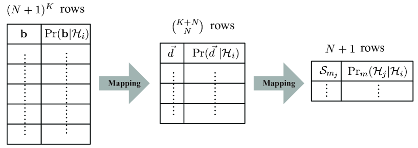
Figure 2: Illustration of mapping from $\mathbf{b}$ to $\vec{d}$ and then to ${\cal S}_{m_{j}}$.

The set ${\cal S}_{m_{j}}$ can be obtained from a mapping function in an offline manner. Hence, we can easily build tables and mapping functions as illustrated in Fig. 2, and compute $\text{Pr}_{m}({\cal H}_{j}|{\cal H}_{i})$ a prior. Fortunately, a more explicit expression for $\text{Pr}_{m}({\cal H}_{j}|{\cal H}_{i})$ in majority voting can be derived as in the following theorem.

Theorem 2

The majority decision fusion has the decision probability,

$$\text{Pr}_{m}({\cal H}_{j}|{\cal H}_{i})$$

$$=\sum_{d_{0}=0}^{\lfloor\frac{K}{2}\rfloor}\sum_{d_{j}=\lceil\frac{K-d_{0}}{N}\rceil}^{K-d_{0}}\sum_{d_{1}=max\{0,\alpha_{1}\}}^{min\{d_{j},\beta_{1}\}}\cdot\cdot\sum_{d_{j-1}=max\{0,\alpha_{j-1}\}}^{min\{d_{j},\beta_{j-1}\}}\sum_{d_{j+1}=max\{0,\alpha_{j+1}\}}^{min\{d_{j}-1,\beta_{j+1}\}}\cdot\cdot\sum_{d_{N}=max\{0,\alpha_{N}\}}^{min\{d_{j}-1,\beta_{N}\}}\!\!\text{Pr}\big{(}\vec{d}|\mathcal{H}_{i}\big{)}$$ (51)

for $j\geq 1$, and

$$\text{Pr}_{m}({\cal H}_{0}|{\cal H}_{i})=\sum_{d_{0}=\lfloor\frac{K}{2}\rfloor+1}^{K}\sum_{d_{1}=0}^{K-d_{0}}\sum_{d_{2}=0}^{K-d_{0}-d_{1}}\ldots\sum_{d_{N-1}=0}^{K-\sum_{l=0}^{N-2}d_{l}}\text{Pr}\big{(}\vec{d}|\mathcal{H}_{i}\big{)},$$ (52)

where $\lceil\cdot\rceil$, and $\lfloor\cdot\rfloor$ denote the ceiling function and floor function, respectively. Moreover, $\alpha_{n}$ and $\beta_{n}$ are defined as

$$\alpha_{n}= \left\{\begin{array}[]{ll}K-\sum_{i=0}^{n-1}d_{i}-(N-n)d_{j}+N-j&\mbox{if $1\leq n<j$}\\ K-\sum_{i=0}^{n-1}d_{i}-(N-n)d_{j}+N-n&\mbox{if $j<n\leq N$}\end{array}\right.,$$ (53)

$$\beta_{n}= \left\{\begin{array}[]{ll}K-\sum_{i=0}^{n-1}d_{i}-d_{j}&\mbox{if $1\leq n<j$}\\ K-\sum_{i=0}^{n-1}d_{i}&\mbox{if $j<n\leq N$}\end{array}\right..$$

Proof:

To calculate the decision probability from (47), we need to find all candidates $\vec{d}$ in ${\cal S}_{m_{j}}$. In other words, we need to determine the range of elements $d_{j}$’s, $j=0,1,\ldots,N$ in $\vec{d}$.

Let us start form $j\geq 1$. As shown in $\mathcal{S}_{m_{j}}$, $\vec{d}$ must satisfy $d_{0}\leq K/2$, so the range of $d_{0}$ should be from $0$ to $\lfloor\frac{K}{2}\rfloor$. Moreover, since $d_{j}=\max\{d_{1},\dots,d_{N}\}$, the lower bound of $d_{j}$ must be no less than $\frac{K-d_{0}}{N}$, otherwise there will always be another $d_{j_{1}}\neq d_{j}$ but satisfies $d_{j_{1}}>d_{j}$. Therefore the range of $d_{j}$ is from $\lceil\frac{K-d_{0}}{N}\rceil$ to $K-d_{0}$. We then separately determine the range of $d_{n}$ for $1\leq n<j$ and $j<n\leq N$, respectively.

1) When $n<j$, the upper bound of $d_{n}$ must be less than or equal to the unassigned value of $K$, which is $K$ minus all the values that have already been assigned to $d_{i},0\leq i<n$ and $d_{j}$, i.e. $K-\sum_{i=0}^{n-1}d_{i}-d_{j}$. Bearing in mind the the constraint $d_{n}\leq d_{j}$, the upper bound can be expressed as

$$d_{n}^{\text{upper}}=\min\left\{d_{j},\ K-\sum_{i=0}^{n-1}d_{i}-d_{j}\right\},\quad n<j.$$

As for the lower bound, $d_{n}$ should not be too small to allow any other undetermined $d_{k}(n<k\leq N$ and $k\neq j)$ be greater than $d_{j}$. The extreme case happens when all the undetermined $d_{k}$’s get their highest values, i.e., $d_{k}$ equals to $d_{j}$ for $n<k<j$ while $d_{k}$ is $d_{j}-1$ for $j<k\leq N$. Then the summation of these $d_{k}$ is $(j-n-1)d_{j}+(N-j)(d_{j}-1)$. Combining this result as well as the constraint $d_{n}\geq 0$, we get the lower bound of $d_{n}$ as

$$d_{n}^{\text{lower}}=\max\left\{K-d_{j}-\sum_{i=0}^{n-1}d_{i}-(j-n-1)d_{j}-(N-j)(d_{j}-1),\ 0\right\},\quad n<j.$$

2) When $n>j$, the maximum value of $d_{n}$ can only be $d_{j}-1$, thus the upper bound of the summand changes to

$$d_{n}^{\text{upper}}=\min\left\{d_{j}-1,\ K-\sum_{i=0}^{n-1}d_{i}\right\},\quad n>j.$$

Similar to the previous discussion, the maximum summation of all the undetermined $d_{k}(n<k\leq N)$ in this situation is $(N-n)(d_{j}-1)$, so the lower bound is

$$d_{n}^{\text{lower}}=\max\left\{K-\sum_{i=0}^{n-1}d_{i}-(N-n)(d_{j}-1),\ 0\right\},\quad n>j.$$

When we use $\alpha_{n}$ and $\beta_{n}$ in (53) to simplify the expression of the range of $d_{n}$’s, the equality (2) for $j\geq 1$ is proved.

As for $j=0$, the only constraint for $\vec{d}$ is $d_{0}>K/2$ from $\mathcal{S}_{m_{j}}$, so the summation range of $d_{0}$ must be from $\lfloor\frac{K}{2}\rfloor+1$ to $N$. All the others $d_{n},n\in\{1,2,\ldots,N\}$ can be freely chosen as long as $\sum_{i=0}^{N}d_{i}=K$. If we assign the values for $d_{i}$’s one by one, then for any $d_{n}$, its lowest possible value is 0 while its highest possible value is $K-\sum_{i=0}^{n-1}d_{i}$. Note that, $d_{N}$ is a fixed value when all the previous $d_{i},0\leq i<N$ are chosen and does not need to be included in the summand. Then, the equality (52) for $j=0$ is proved. ∎

Once $\text{Pr}_{m}({\cal H}_{j}|{\cal H}_{i})$ is derived, then the false alarm, the detection probability as well as the discrimination probability for majority cooperation can be immediately obtained as the summation of corresponding $\text{Pr}_{m}({\cal H}_{j}|{\cal H}_{i})$.

Remark 14

Though majority decision fusion rule has been widely accepted in many research areas, the analytical approach to study its performance, e.g, obtaining $\text{Pr}_{m}({\cal H}_{j}|{\cal H}_{i})$ from $\text{Pr}({\cal H}_{j}|{\cal H}_{i})$, has never been fully discussed to the best of the authors’ knowledge.

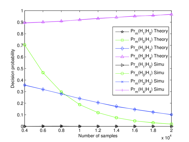
Figure 3: Theoretical analysis and numerical results for decision probability under majority decision fusion.

In Fig. 3, we provide one example to verify several $\text{Pr}_{m}({\cal H}_{j}|{\cal H}_{i})$ with $N=4$, $K=5$ and average SNR=$-12$dB. It is clearly seen that the numerical results match the theoretical ones very well.

IV-B Optimal Decision Fusion

Though the majority decision fusion rule is very simple and effective, it does have some drawbacks which limit the performance. For example, when $\text{Pr}({\cal H}_{i})\gg\text{Pr}({\cal H}_{j})$, even if the detection result is $d_{i}<d_{j}$, it is still possible that ${\cal H}_{i}$ is truer than ${\cal H}_{j}$. The reason is that majority decision is a type of ‘hard” decision and is not “soft” enough to count in the prior probability of each hypothesis.

From the probabilistic point of view, the optimal decision fusion with the observation $\vec{d}$ should follow MAP criterion [30]. Similar to majority decision fusion, we need to first to make a decision about the presence of PU before recognizing the power levels, i.e.,

$$\text{Pr}\big{(}\mathcal{H}_{\text{off}}|\vec{d}\ \big{)}\mathop{\gtrless}\limits_{\mathcal{H}_{\text{on}}}^{\mathcal{H}_{\text{off}}}\text{Pr}\big{(}\mathcal{H}_{\text{on}}|\vec{d}\ \big{)}.$$ (54)

From Bayes rule, there is

$$\text{Pr}\big{(}{\cal H}_{n}|\vec{d}\ \big{)}=\frac{\text{Pr}\big{(}\vec{d}\ |{\cal H}_{n}\big{)}\text{Pr}({\cal H}_{n})}{\text{Pr}\big{(}\vec{d}\ \big{)}}.$$ (55)

Hence, (54) can be simplified as

$$\text{Pr}\big{(}\vec{d}\ |\mathcal{H}_{0}\big{)}\text{Pr}(\mathcal{H}_{0})\mathop{\gtrless}\limits_{\mathcal{H}_{\text{on}}}^{\mathcal{H}_{\text{off}}}\sum_{i=1}^{N}\text{Pr}\big{(}\vec{d}\ |\mathcal{H}_{i}\big{)}\text{Pr}(\mathcal{H}_{i}).$$ (56)

If PU is detected to be present, we continue to recognize the power level of PU. Following the similar steps from (12) to (16), the detection rule is

$$\hat{i}=\arg\max_{i\geq 1}\ \text{Pr}\big{(}{\cal H}_{i}|\vec{d}\ \big{)}=\arg\max_{i\geq 1}\ \text{Pr}\big{(}\vec{d}\ |{\cal H}_{i}\big{)}\text{Pr}({\cal H}_{i}).$$ (57)

The decision probability of the optimal decision fusion can be expressed as

$$\text{Pr}_{o}({\cal H}_{j}|{\cal H}_{i})=\sum_{\vec{d}\in{\cal S}_{o}}\text{Pr}(\vec{d}\ |{\cal H}_{i})$$ (58)

where the set ${\cal S}_{o_{j}}$ is defined as

$${\cal S}_{o_{j}}= \left\{\begin{array}[]{ll}\{\vec{d}\ \big{|}\ \text{those}\ \vec{d}\ \text{that claim absence from}\ (\ref{eq:opt fusion})\}&\mbox{if $j=0$}\\ \{\vec{d}\ \big{|}\ \text{those}\ \vec{d}\ \text{that result in}\ \hat{i}=j\ \text{in}\ (\ref{eq:opti})\ \text{but claim presence from}\ (\ref{eq:opt fusion})\}&\mbox{if $j\geq 1$}\end{array}\right.$$

The elements in ${\cal S}_{o_{j}}$ is an implicit function of $\text{Pr}({\cal H}_{i})$ and $\text{Pr}({\cal H}_{j}|{\cal H}_{i})$, which makes it difficult to obtain an explicit expression of $\text{Pr}_{o}({\cal H}_{j}|{\cal H}_{i})$. Nevertheless, $\text{Pr}_{o}({\cal H}_{j}|{\cal H}_{i})$ is the summation of those $\text{Pr}(\vec{d}\ |{\cal H}_{i})$ whose $\vec{d}$ could result in the decision of $j$ and these $\vec{d}$ can be found from a predetermined mapping, as did in Fig. 2.

Remark 15

Since $\text{Pr}({\cal H}_{i})$ and $\text{Pr}({\cal H}_{j}|{\cal H}_{i})$ are real continuous values, the probability for obtaining more than one maximum index from (57) is 0, and the corresponding discussion is not necessary.

Remark 16

If we assume the same fading gain for all SUs [10] and apply (13), then a more concise form of the decision (57) can be obtained as

$$\hat{i}= \arg\max_{i\geq 1}\ \text{Pr}({\cal H}_{i})\prod_{n=0}^{N}\text{Pr}({\cal H}_{n}|{\cal H}_{i})^{d_{n}}=\arg\max_{i\geq 1}\ \log\text{Pr}({\cal H}_{i})+\sum_{n=0}^{N}d_{n}\log\text{Pr}({\cal H}_{n}|{\cal H}_{i}).$$ (59)

V Simulations

In this section, we resort to numerical examples to evaluate the proposed studies. Four levels of primary transmit power are assumed, while the corresponding prior probabilities are set as $\text{Pr}({\cal H}_{0})=0.5$, and $\text{Pr}({\cal H}_{i})=0.125,i=1,2,3,4$. The channel gain $\gamma$ and the noise variances are taken as units. The power levels satisfy $P_{1}:P_{2}:P_{3}:P_{4}=3:5:7:9$, and the average SNR is defined as $\frac{1}{4}\sum_{i=1}^{4}P_{i}/{\sigma^{2}_{n}}$.

V-A Sensing with A Single SU

In Fig. 4, we evaluate the performance of detecting the presence of PU versus the number of samples for the proposed sensing strategies. It is seen that sensing strategy-I works better than sensing strategy-II, especially when the sampling number is small, which matches our discussion in Section III-C that $\theta_{\text{on/off}}<\phi_{\text{on/off}}$. Nevertheless, the gaps between the two sensing strategies reduce when the number of samplings become larger or the PU’s SNR becomes higher. This implies that when the sensing conditions becomes better, then difference of the two sensing strategies gradually diminishes and the choice of sensing strategies becomes less important.

One the other hand, Fig. 5 displays the performance of discriminating the power level versus the number of samples of the proposed sensing strategies. The discrimination probability follows the definition in (36), i.e., we treat absence as an equivalent power level with 0 value. From Fig. 5, we see that sensing strategy-II works slight better than strategy-I but the difference diminishes when SNR becomes higher. This phenomenon right fits our analysis in subsection III-C that strategy-II takes into account all error cases.

Next we demonstrate the sensing performance versus SNR in Fig. 6 for both the detection probability and the discrimination probability defined in (29). It is seen that sensing strategy-I out performs sensing strategy-II in terms of both detection probability and discrimination probability. For sensing strategy-I, the difference between detection probability and discrimination probability is very large at low SNR. The reason is that even if PU is detected to be present, the strategy-I actually makes many mistakes about PU’s actual power level. However, for sensing strategy-II, $\mathcal{H}_{0}$ may mask all the other states when SNR is low, which almost ruins the detecting ability. Nevertheless, since sensing strategy II is originally defined for discriminating all $\mathcal{H}_{i},i\geq 0$, once we include $\mathcal{H}_{0}$, the discrimination probability could outperform sensing strategy-I as has been demonstrated in Fig. 5.

V-B Cooperative Sensing

For cooperative sensing examples, the local sensing results of all users are made from strategy-I.

In Fig. 7, we show the detection probability as well as the discrimination probability versus the number of receive samples when five SUs cooperative to make the final decision. The SNR is taken as -12 dB. Compared with the sensing performance of single local SU in Fig. 4 and Fig. 5, it is clearly seen that the performance is greatly improved when cooperative scheme is applied. Moreover, the optimal decision outperforms the majority decision at all sample numbers. Nevertheless, the optimal decision needs to dynamically build the mapping function and is not as simple as the majority decision fusion.

The average error detection probability of the two fusion rules versus the number of samples is displayed in Fig. 8. Five SUs cooperate to make the final decision and SNR is taken as -12 dB. Moreover, $\delta$ denotes the offset of index between the true power level and the detected power level, e.g., the detection error probability with $\delta=1$ is the summation of those $\text{Pr}({\cal H}_{j}|{\cal H}_{i})\text{Pr}(\mathcal{H}_{i})$ satisfying $|i-j|=1$, i.e., $\sum_{|i-j|=1}\text{Pr}({\cal H}_{j}|{\cal H}_{i})\text{Pr}(\mathcal{H}_{i})$. It is seen that the error probability decreases extensively when $\delta$ increases. This is not unexpected because the chances for making a wrong decision to the farer power level should be smaller. A very important indication to practical design is that, SUs may only pay attention to those errors with smaller $\delta$ and set the corresponding cost values in Bayes Risk detection.

Next we show the performance of cooperative sensing versus SNR in Fig. 9. Not surprisingly, the optimal decision fusion rule outperforms the majority decision fusion in all SNR range. Besides, the discrimination probability for both sensing rules also get closer to the detection probability as the SNR grows. Moreover, the gaps between the optimal fusion and the majority fusion diminish when SNR becomes larger.

In the last example, we show the detection probability and discrimination probability versus the number of SU in Fig. 10, with SNR$=-12$dB and $M=5000$. Obviously, both decision rules provide better results when the number of the SUs increases and the optimal decision rule always outperforms the majority rule, which matches our intuition very well. Moreover, increasing the number of SU after a certain amount may not be very helpful, e.g., eight SUs in majority sensing strategy.

VI Conclusions

In this paper, we investigated a new CR scenario, i.e., MPTP, that embraces multiple primary powers, which both matches the practical transmission and fits the theocratical demands of adapting the transmit power. We designed two different spectrum sensing strategies which are shown to possess different but correlated optimization criteria. Most results, e.g., threshold expressions, probabilities, are derived in closed-forms. We present a thorough discussion over all kinds of aspects of the new spectrum sensing strategies, including the power mask effects and its reasoning, the new definition of performance metrics, as well as the rationales behind. Moreover, we developed two different cooperative sensing algorithms which are shown to be very different from the traditional cooperative schemes. Various simulations are provided lately to corroborate the proposed studies. It is then believed that there could exist many new problems in MPTP waiting for exploitation, while in the mean time, many existing studies for traditional CR deserve re-investigation.

TABLE I: Protected Service Contour Levels

Type of TV	Band/Channel	Protected
station		Contour E-field
		Level(dBu)
Full Power	Low VHF (2-6)	47
Analog TV	High VHF (7-13)	56
	UHF (14-69)	64
Low Power	Low VHF (2-6)	62
Analog TV	High VHF (7-13)	68
	UHF (14-69)	74
Full Power	Low VHF (2-6)	28
Digital TV	High VHF (7-13)	36
	UHF (14-51)	41
Low Power	Low VHF (2-6)	43
Digital TV	High VHF (7-13)	48
	UHF (14-51)	51

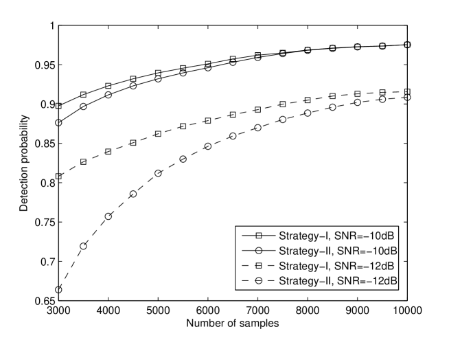
Figure 4: The detection probability of local SU versus the number of samples with average SNR$=-10\text{dB},-12\text{dB}$.

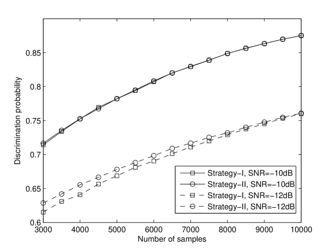
Figure 5: The discrimination probability of local SU versus the number of samples.

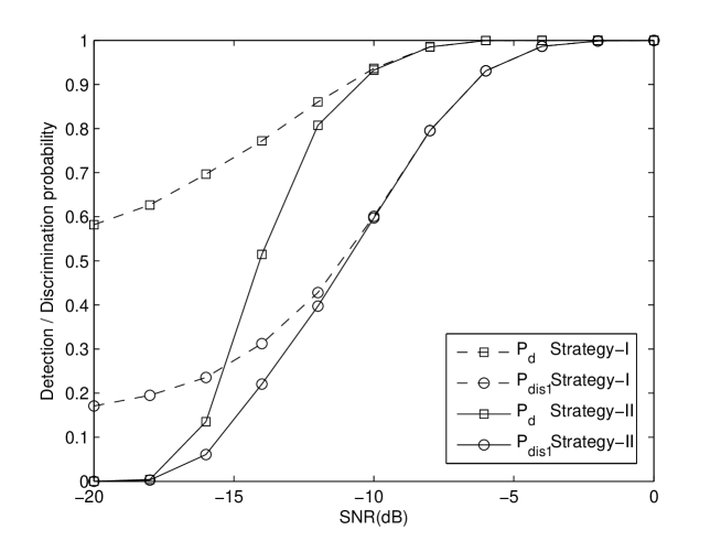
Figure 6: The detection and discrimination probability of local SU versus SNR with M=5000.

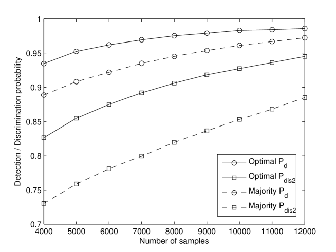
Figure 7: Detection probability and discrimination probability versus number of samples for these two cooperative sensing methods with $K=5$, SNR$=-12$dB.

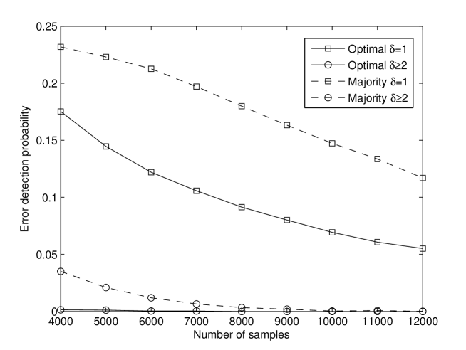
Figure 8: Error detection probability versus the number of samples for $K=5$, SNR$=-12$dB.

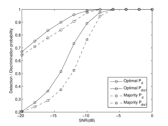
Figure 9: Detection probability and discrimination probability in cooperative sensing versus SNR with $K=5$, $M=5000$.

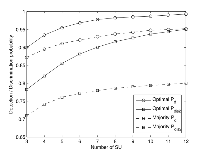
Figure 10: Detection probability and discrimination probability versus the number of SU for SNR$=-12$dB, $M=5000$.

References

- [1] S. Haykin, “Cognitive radio: brain-empowered wireless communications,” IEEE J. Select. Areas Commun., vol. 23, pp. 201–220, Feb. 2005.
- [2] R. Tandra and A. Sahai, “Fundamental limits on detection in low SNR under noise uncertainty,” in Proc. IEEE Int. Conf. Wireless Networks, Commun. and Mobile Computing, vol. 1, Maui, HI, June 2005, pp. 464–469.
- [3] S. Shankar, C. Cordeiro, and K. Challapali, “Spectrum agile radios: utilization and sensing architectures, in Proc. IEEE Int. Symposium on New Frontiers in Dynamic Spectrum Access Networks, Baltimore, Maryland, USA, Nov. 2005, pp. 160–169.
- [4] T. Yucek and H. Arslan, “A survey of spectrum sensing algorithms for cognitive radio applications,” IEEE Commun. Survey & Turtorials, vol. 11, no. 1, First Quater, 2009.
- [5] Y. Li and S. K. Jayaweera, “Dynamic spectrum tracking using energy and cyclostationarity-based multi-variate non-parametric quickest detection for cognitive radios, IEEE Trans. Wireless Commun., vol. 12, no. 7, pp. 3522–3532, July 2013.
- [6] D. Cabric, S. M. Mishra, and R. W. Brodersen, “Implementation issues in spectrum sensing for cognitive radios,” in Proc. Asilomar Conf. on Signals, Systems, and Computers, Pacific Grove, California, USA, Nov.7-10, 2004, pp. 772–776.
- [7] P. Urriza, E. Rebeiz, and D. Cabric, “Multiple antenna cyclostationary spectrum sensing based on the cyclic correlation significance test,” IEEE J. Select. Areas in Commun., vol. 29, no. 2, pp. 362–373, vol. 31, no. 11, pp. 2185–2195, Oct. 2013.
- [8] Y. Zeng, and Y.-C. Liang, “Eigenvalue-based spectrum sensing algorithms for cognitive radio,” IEEE Trans. Commun., vol. 57, no. 6, pp. 1784–1793, June 2009.
- [9] S. Sedighi, A. Taherpour, and J. Sala, “Spectrum sensing using correlated receiving multiple antennas in cognitive radios,” IEEE Trans. Wireless Commun., accepted.
- [10] W. Zhang, R. K. Mallik, and K. B. Letaief, “Optimization of cooperative spectrum sensing with energy detection in cognitive radio networks,” IEEE Trans. on Wireless Commun., vol. 8, no. 12, pp. 5761–5766, Dec. 2009.
- [11] E. C. Y. Peh, and, Y.-C. Liang, Y. L. Guan, and Yonghong Zeng, “Cooperative spectrum sensing in cognitive radio networks with weighted decision fusion schemes,” IEEE Trans. Wireless Commun., vol. 9, no. 12, pp. 3838–3947, Dec. 2010.
- [12] W. Han, J. Li, Z. Li, and J. Si, “Efficient soft decision fusion rule in cooperative spectrum sensing,” IEEE Trans. Signal Processing, vol. 61, no. 8, pp. 1931–1943, Mar. 2013.
- [13] J. Font-Segura and X. Wang, “GLRT-based spectrum sensing for cognitive radio with prior information,” IEEE Trans. Commun., vol. 58, no. 7, pp. 2137–2146, July 2010.
- [14] Z. Zhang, H. Jiang, P. Tan, and J. Slevinsky, “Channel exploration and exploitation with imperfect spectrum sensing in cognitive radio networks,” IEEE J. Select. Areas in Commun., vol. 31, no. 3, pp. 429–441, Feb. 2013.
- [15] Y.-C. Liang, Y. Zeng, C.Y. Peh, and A. T. Hoang, “Sensing-throughput tradeoff for cognitive radio networks,” IEEE Trans. Wireless Commun., vol. 7, no. 3, pp. 1326–1337, Mar. 2008.
- [16] X. Kang, Y.-C. Liang, H. K. Garg, and L. Zhang,“Sensing-based spectrum sharing in cognitive radio networks,” IEEE Trans. Veh. Tech., vol. 58, no. 8, pp. 4649–4654, Oct. 2009.
- [17] Y. J. Zhang and A.M.-C. So, “Optimal spectrum sharing in MIMO cognitive radio networks via semidefinite programming,” IEEE J. Select. Areas in Commun., vol. 29, no. 2, pp. 362–373, Jan. 2011.
- [18] G. Scutari and J.-S. Pang, “Joint sensing and power allocation in nonconvex cognitive radio games: nash equilibria and distributed algorithms,” IEEE Trans. Inf. Theory, vol. 59, no. 7, pp. 4626–4661, July 2013.
- [19] Y. Zeng, Y.-C. Liang and H. Pham, “Spectrum sensing for OFDM signals using pilot induced auto-correlations,” IEEE J. Select. Areas in Commun., 31, no. 3, pp. 353–363, Mar. 2013.
- [20] Y. Zou, Y.-D. Yao and B. Zheng, “Cooperative relay techniques for cognitive radio systems: spectrum sensing and secondary user transmissions,” IEEE Commun. Mag., vol. 50, no. 4, pp. 98–103, Apr. 2012.
- [21] Wireless LAN Medium Access Control (MAC) and Physical Layer (PHY) Specifications, IEEE std 802.11, 1999.
- [22] European digital cellular telecommunication system (Phase 2), ETSI, 1995.
- [23] 3GPP TS 36.213, Evolved Universal Terrestrial Radio Access (EUTRA), “User Equipment (UE) Radio Transmission and Reception,” (release 8).
- [24] 3GPP TR 36.913, “Requirements for Further Advancements for Evolved Universal Terrestrial Radio Access (E-UTRA) (LTE-Advanced),” 3GPP, Tech. Rep. v. 10.0.0, Mar. 2011,
- [25] D. Catrein, L. A. Imhof, and R. Mathar, “Power control, capacity, and duality of uplink and downlink in cellular CDMA systems,” IEEE Trans. Commun., vol. 52, no. 10, pp. 1777–1785, Oct. 2004.
- [26] C. Y. Wong, R.S. Cheng, K. B. Lataief, and R. D. Murch, “Multiuser OFDM with adaptive subcarrier, bit, and power allocation,” IEEE J. Select. Areas in Commun., 17, no. 10, pp. 1747–1758, Oct. 1999.
- [27] Q. Cao, Y. Jing, and H. V. Zhao, “Power allocation in multi-user wireless relay networks through bargaining,” IEEE Trans. Wireless Commun., vol. 12, no. 6, pp. 2870–2882, June 2013.
- [28] G. Ganesan and Y. Li, “Cooperative spectrum sensing in cognitive radio-partII: multiuser networks,” IEEE Trans. Wireless Commun., vol. 6, no. 6, pp. 2214–2222, June 2007.
- [29] C. Zhong, F. Gao, X.-D. Zhang, C. F. Li, and M. Lei, “Sensing and power allocation for cognitive radio with multiple primary transmit powers,” IEEE Wireless Commun. Lett., vol. 2, no. 3, pp. 319–322, June 2013.
- [30] S. M. Kay, Fundamentals of Statistical Signal Processing: Detection Theory. Prentice Hall PTR, 1993.
- [31] In the Matter of Unlicensed Operation in the TV Broadcast Bands, ET Docket No. 04-186, Notice of Proposed Rulemaking, FCC OET, May 2004.