On the origin of the featureless soft X-ray excess emission from the Seyfert 1 galaxy ESO 198–G24.

Abstract

We present medium and high resolution X-ray spectral study of a Seyfert 1 galaxy ESO 198–G24 using a long ($\sim 122\,\rm ks$) XMM-Newton observation performed in February 2006. The source has a prominent featureless soft X-ray excess below $2\rm\,\,{\rm keV}$. This makes the source well suited to investigate the origin of the soft excess. Two physical models – blurred reflection, and optically thick thermal Comptonization in a warm plasma, describe the soft-excess equally well resulting in similar fits in the $0.3-10\rm\,\,{\rm keV}$ band. These models also yield similar fits to the broad-band UV (Optical Monitor) and X-ray data. XMM-Newton observations performed in 2000, 2001 and 2006 on this source show flux variability. From 2001 to 2006, the UV flux increased by $\sim 23\%$ while the $2-10\rm\,\,{\rm keV}$ X-ray flux as well as the soft-excess flux decreased by $\sim 20\%$. This observation can be described in the blurred reflection scenario by a truncated accretion disk whose inner-most radius had come closer to the blackhole. We find that the best-fit inner radius of the accretion disk decreases from $\rm R_{in}=4.93_{-1.10}^{+1.12}R_{G}$ to $\rm R_{in}<2.5R_{G}$ from 2001 to 2006. This leads to an increase in the UV flux and compressing the corona, leading to reduction of the powerlaw flux and therefore the soft-excess. The blurred reflection model seems to better describe the soft-excess for this source.

1 Introduction

Many Seyfert 1 galaxies show a prominent soft X-ray excess (SE) emission over and above a powerlaw component extending to high energies. This SE was first detected by Pravdo et al. (1981) using HEAO-1 data and also by Arnaud et al. (1985) and Singh et al. (1985) using EXOSAT data. The nature and origin of the SE is still uncertain. In most cases it is well described by blackbody or multiple blackbody emission with photon temperature ranging from $0.1-0.2\rm\,\,{\rm keV}$ over several decades in AGN mass (Gierliński & Done, 2006). If one assumes this feature to have a thermal origin, then its temperature is quite high as compared to that predicted by the standard accretion disk model of Shakura & Sunyaev (1973). The constancy of the temperature of the SE points to the fact that its origin is likely related with the atomic physics, in a way that the shape of the SE is the result of atomic transitions. The SE can be described as blurred reflection from a partially ionised accretion disk when a hard X-ray photon flux is incident on it (Ross & Fabian, 2005). It can also be physically explained by Comptonisation of disk photons by an optically thick electron cloud at higher temperature (Done et al., 2012). The soft excess is usually modified by the presence of strong and complex warm absorber features. This makes the characterization of both the soft excess and the warm absorbers difficult particularly if the spectral resolution is moderate or the signal to noise ratio is low. Therefore, it is important to study Seyfert 1 galaxies without significant soft X-ray warm absorber or other features in order to probe the nature of SE emission. The Seyfert 1 galaxy ESO 198–G24 is one such AGN with featureless soft X-ray excess.

ESO 198–G24 was observed in the soft X-ray band by ROSAT twice during $1991-1992$ (Turner et al., 1993). It was noted that the spectrum had varied between the two observations. There was a flattening of the soft X-ray spectrum, and the emission lines and absorption edges were not required statistically in the second 1992 observation. It was possible to put a lower limit on the variability time scale of six months.

Guainazzi (2003) studied ESO 198–G24 using the $\sim 40\,\rm ks$ data from ASCA (1997), $\sim 9\,\rm ks$ data from XMM-Newton (2000), and $\sim 150\,\rm ks$ from BeppoSAX (2001). The study revealed that the Fe K$\alpha$ line profile and the line intensity varied between the observations. In the XMM-Newton data, Guainazzi (2003) found an additional emission line feature at $5.7\rm\,\,{\rm keV}$ with an equivalent width $70\pm 40\,{\rm\,eV}$ and suggested that it might be a part of the double horned profile of the Fe line.

Porquet et al. (2004) studied the source using an XMM-Newton observation performed in 2001. There was no clear evidence of warm absorption in the soft X-ray band, however there were weak relativistic emission lines of OVIII and CVI Ly$\alpha$ in the RGS data. An FeK$\alpha$ line at $6.41\rm\,\,{\rm keV}$ with an equivalent width of about $60-70\,{\rm\,eV}$ was clearly detected. As a part of a sample study, Tombesi et al. (2010) have investigated the presence of high ionisation outflows from ESO 198–G24 using data obtained from an XMM-Newton observation in 2006. They did not find any narrow absorption line in the Fe K band, however they found a narrow absorption edge at $4.59\rm\,\,{\rm keV}$. It could possibly be associated with Ca xx Ly $\alpha$, blueshifted by a velocity of $\sim 0.1$c. de Marco et al. (2009) studied the source as a part of a sample study investigating the variability of the Fe K complex. They used the time averaged spectrum from $4-9\rm\,\,{\rm keV}$, and found that the Fe K$\alpha$ line varied between the two XMM-Newton observations in 2001 and 2006, in that the former data showed a broader Fe K$\alpha$ line with an upper limit on the line width $\sigma<0.36\rm\,\,{\rm keV}$. They also found an absorption line in the 2006 XMM-Newton data at $7.56\rm\,\,{\rm keV}$ with an equivalent width of $40\,{\rm\,eV}$.

In this paper we make a detailed broadband spectral study of ESO 198–G24 using all the available XMM-Newton datasets and investigate the origin of the soft X-ray excess emission. This is the first detailed spectral analysis for this long $122$ ks dataset. Section 2 describes the observations and data reduction. Section 3 deals with broad band spectral analysis (EPIC-pn and OM+EPIC-pn), as well as RGS spectral analysis. We discuss our results in section 4 followed by the conclusions.

Table 1: The three XMM-Newton observations of ESO 198–G24 used in this work.

Observation	Observation	Observation	Total exposure
number	id	date	time
1	0112910101	2000-12-01	13 ks
2	0067190101	2001-01-24	34 ks
3	0305370101	2006-02-04	122 ks

2 Observation & Data Reduction

ESO 198–G24 was observed by XMM-Newton on three occasions in December 2000, January 2001 and February 2006 for $13$, $43$ and $122\,\rm ks$, respectively (see Table 1 for details). We have analysed in detail the data obtained from the long $122\,\rm ks$ observation on 2006 (observation number 3, see Table 1). In this observation, the EPIC-pn camera was operated in the small window mode and the MOS cameras were operated in the partial window mode. Data were reduced using SAS version 11.0.0.

We processed the EPIC-pn and MOS data with epchain and emchain respectively, and filtered them using the standard filtering criterion. Examination of the background rate above 10 keV showed that the observation was partly affected by a flaring particle background at the beginning of the observation upto an elapsed time of $5\,\rm ks$. We checked for the photon pile-up using the SAS task epatplot and found that there were no noticeable pile-up in either EPIC-pn or MOS data. We quote results based on EPIC-pn data due to its higher signal-to-noise compared to the MOS data. We have used single pixel events with pattern=0 and FLAG=0. To extract the source spectrum and lightcurve, we chose a circular region of $43{\rm~{}arcsec}$, centred on the centroid of the source. For background spectrum and lightcurve, we used nearby circular regions that are free of any sources. Figure 1 shows the background-corrected light curves of the source in the soft ($0.2-2\rm\,\,{\rm keV}$) and hard X-ray ($2-10\rm\,\,{\rm keV}$) bands along with the hardness ratio. We used the full length of the observation to extract the lightcurves. The net source light curve was obtained after appropriate background subtraction using FTOOLS task lcmath. We note that the hardness-ratio has not varied significantly within the observation. We created the ancillary response file (ARF) and the redistribution matrix file (RMF) using the SAS tasks arfgen and rmfgen, respectively. After filtering, the net exposure in the EPIC-pn data is $85\,\rm ks$, and the net counts is $4\times 10^{5}$.

We processed the RGS data using the SAS task rgsproc. We chose a region, CCD9, that is most susceptible to proton events and generally records the least source events due to its location close to the optical axis and extracted the background light curve. We then generated a good time interval file to filter the eventlist and extracted the first order source and background spectrum.

We processed the optical monitor (OM) data using omichain. We obtained the count rates in 5 active filters by specifying the RA and Dec of the source in the source list file obtained by the omichain task. The count rate thus obtained was converted to flux using standard tables. See section 3.3 for details. For variability studies (section 3.4), we have also analysed the OM and EPIC-pn datasets from two earlier XMM-Newton observations, for which we follow the same procedure as described above for data reduction. There was no pile up in the data for these observations. The hardness ratio of the source was found to be constant during these two observations.

Figure 1: Background subtracted EPIC-pn lightcurves of ESO 198–G24 in the soft ($0.2-2\rm\,\,{\rm keV}$) band (top panel), in the hard ($2-10\rm\,\,{\rm keV}$) band (middle panel), and the hardness ratio (bottom panel) for observation 3 (id:0305370101).

.

3 Spectral Analysis

We grouped the EPIC-pn spectral data with a minimum of 20 counts per energy bin and at most 5 energy bins per resolution element, using the specgroup command in the SAS. We used ISIS version 1.6.1-36 (Houck & Denicola, 2000) for our spectral fitting. All errors quoted on the fitted parameters reflect the $90\%$ confidence interval.

We begin with the spectral analysis of the $2-10\rm\,\,{\rm keV}$ data. A simple powerlaw model with absorption due to neutral column in our Galaxy (wabs) provided a $\rm\chi^{2}/dof=292/198\sim 1.50$, where dof stands for degrees of freedom. The best fit equivalent neutral Hydrogen column density, $\rm N_{H}\leq 3\times 10^{20}\rm\,\,{\rm cm^{-2}}$, is consistent with the Galactic column ($\rm N_{H}^{Gal}=2.93\times 10^{20}\rm\,\,{\rm cm^{-2}}$; Kalberla et al., 2005), and therefore we fixed $\rm N_{H}$ to this value. There was no evidence for an additional neutral absorber intrinsic to the source. The best fit powerlaw slope was $\Gamma=1.64_{-0.01}^{+0.04}$. Figure 2 shows the $2-10\rm\,\,{\rm keV}$ spectrum fitted with an absorbed powerlaw model, and the ratio of the observed data and the model. There are two emission lines at $\sim 6.4\rm\,\,{\rm keV}$ and $\sim 7\rm\,\,{\rm keV}$ in the rest frame ($z=0.0455$) and also there are weak absorption features at $\sim 7.4\rm\,\,{\rm keV}$. The Fe K$\alpha$ feature has been detected previously in the same dataset as a part of sample study by Tombesi et al. (2010) and de Marco et al. (2009).

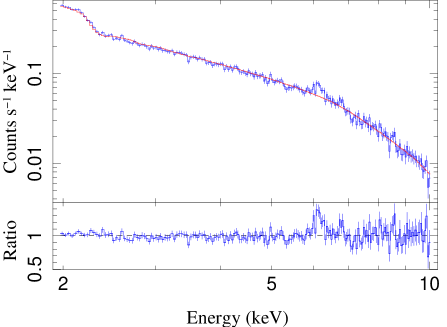
Figure 2: The $2-10\rm\,\,{\rm keV}$ EPIC-pn data fitted by a simple absorbed powerlaw model to show the Fe K line complex in the energy range of $6-8\rm\,\,{\rm keV}$ (observer’s frame). FeK$\alpha$ and K$\beta$ emission lines and weak FeK absorption lines are visible in the residuals.

We used a Gaussian profile to fit the prominent Fe K$\alpha$ emission line at $6.4\rm\,\,{\rm keV}$. The best fit line energy is $6.41_{-0.05}^{+0.04}\rm\,\,{\rm keV}$. Initially we fixed the standard deviation of the Gaussian line, $\sigma$, to a value $0.01\rm\,\,{\rm keV}$ and found a weak red wing with $\,\rm\chi^{2}/dof=229/194$. Then we allowed the $\sigma$ to vary and the fit improved to $\,\rm\chi^{2}/dof=213/193$. We found that the Gaussian line was slightly broader than the instrumental resolution with $\sigma=0.12_{-0.04}^{+0.01}\rm\,\,{\rm keV}$, which corresponds to an FWHM speed of $13000_{-4250}^{+1000}\rm\,\,{\rm km\,s^{-1}}$. The equivalent width of the line is $78\pm 20\,{\rm\,eV}$. We then checked for a possible relativistically broadened iron line component around $6\rm\,\,{\rm keV}$ with an ISIS additive model laor (Laor, 1991). We allowed the emissivity index of the model to vary between $2-4$, so that we got dominant flux from the inner regions of the accretion disk compared to the outer regions, thus giving rise to a broad component. We found that the addition of this component did not improve the fit statistically. Previous studies on this source by de Marco et al. (2009); Porquet et al. (2004); Guainazzi (2003) also did not find any broad underlying feature. Guainazzi (2003) however detected an emission line at $5.7\rm\,\,{\rm keV}$ which he interpreted as the red horn of the FeK line profile. Shu et al. (2010) had studied the Chandra data of the source and found a narrow FeK$\alpha$ line at $6.4\rm\,\,{\rm keV}$. We also found weak positive residuals at $7.05\rm\,\,{\rm keV}$ which when modeled with a narrow Gaussian improved the fit by $\,\Delta\chi^{2}=-17$ for 3 new parameters to $\,\rm\chi^{2}/dof=196/190$. The narrow absorption line when modeled with an inverted narrow Gaussian, improved slightly the fit to $\,\rm\chi^{2}/dof=189/187$ with a line centre energy of $7.45_{-0.07}^{+0.07}$. The fit seemed satisfactory in the $2-10\rm\,\,{\rm keV}$ regime which we extrapolated to the lower energies.

On extrapolating the above best-fit model to the whole band ($0.3-10\rm\,\,{\rm keV}$), we found a clear presence of soft X-ray excess emission below $2\rm\,\,{\rm keV}$. The origin of such soft excess in type 1 AGNs is still unclear. Several models such as single or multiple blackbodies, multicolor disk blackbody, blurred reflection from partially ionised material, smeared absorption, and thermal Comptonization in an optically thick medium can provide statistically good fit to the observed soft excess (Magdziarz et al., 1998; Fabian et al., 2002; Gierliński & Done, 2004; Porquet et al., 2004; Crummy et al., 2006; Dewangan et al., 2007). We fitted the soft excess with a simple phenomenological bbody model and still found some positive residuals in the soft X-rays for which we used one more bbody model and the fit statistics improved from $\rm\chi^{2}/dof=1806/257$ to $\rm\chi^{2}/dof=382/253$. The model used in ISIS terminology is wabs$\times$(bbody(1)+bbody(2)+powerlaw+Gaussian(1)+
Gaussian(2)-Gaussian(3)). The best fit blackbody temperatures obtained were $\rm kT_{BB}=0.08\pm 0.02\rm\,\,{\rm keV}$ and $\rm kT_{BB}=0.17\pm 0.07\rm\,\,{\rm keV}$. The fit statistic of $\chi^{2}_{\nu}\sim 1.51$ was unacceptably high which may possibly be due to a cold reflection continuum present at energies $>4\rm\,\,{\rm keV}$. This continuum emission originates from blurred reflection of hard X-ray photons off a neutral medium distantly located from the blackhole, possibly in the torus or the broad line region. We used the PEXRAV model (Magdziarz & Zdziarski, 1995) which gives us the direct powerlaw emission as well as the reflection from the cold disk to model this feature, and that improved the fit by $\,\Delta\chi^{2}=-118$ to $\,\rm\chi^{2}/dof=264/250$. The best fit parameters are listed in Table 2. Given the small band pass of the XMM-Newton in the hard X-ray range, the relative reflection coefficient (R) of PEXRAV however could not be properly estimated, with a value of $2.27_{-0.5}^{+0.7}$.

The neutral and narrow iron K$\alpha$ line and Compton reflection from neutral material could physically arise from the same component. Therefore a single model describing them together would better constrain the parameter values. We therefore removed the cold reflection model PEXRAV and the Gaussian line at $6.4\rm\,\,{\rm keV}$, and used the model PEXMON (Nandra et al., 2007) that combines the cold reflection PEXRAV with self-consistently generated Fe K$\alpha$, Fe K$\beta$, Ni K$\alpha$, Fe K$\alpha$ and the Compton shoulder. To achieve this, the $0.3-10\rm\,\,{\rm keV}$ spectrum was fitted with the model wabs$\times$(bbody(1)+bbody(2)+powerlaw+PEXMON-Gaussian), in ISIS notation. We ensured that PEXMON models only the reflection component and not the direct powerlaw. The $\Gamma$ and the norm of PEXMON were tied to the corresponding parameters of powerlaw. The best fit value of the reflection coefficient R is $-1.16_{-0.20}^{+0.31}$ and the Fe abundance is $0.27_{-0.07}^{+0.10}$ which seems to be well constrained.

At $7.40\rm\,\,{\rm keV}$ we have earlier detected an absorption line. Such a line had been identifed as highly ionised absorption from Fe by several authors e.g, Chartas et al. (2003); Pounds et al. (2003); Braito et al. (2007). We removed the inverted Gaussian and used a warm absorber table model generated using a photoionisation code XSTAR (Kallman et al., 2004), which improved the fit by $\,\Delta\chi^{2}=-8$ for 3 extra parameters to $\,\rm\chi^{2}/dof=273/253$. The ionisation parameter derived from the best fit was $\log\xi=2.87_{-0.14}^{+0.05}$, the column density was $5.15_{-4.0}^{+5.1}\times 10^{21}\rm\,\,{\rm cm^{-2}}$, and the outflow velocity calculated with respect to the systemic velocity was $\sim\rm 0.1c$, which shows that we detect a highly ionised, high velocity outflow. Since the detection is weak, we carried out a Monte-Carlo simulation to test the significance of this absorption feature. The Monte-Carlo test suggests that the absorption features are detected at $<2\sigma$ significance. Tombesi et al. (2010) did not detect the absorption features in the same dataset as they have adopted a criteria where only those features with Monte Carlo derived confidence levels $\geq 95\%$ are selected.

We also tested for the presence of warm absorbers in the energy band $0.3-2\rm\,\,{\rm keV}$ using a low ionisation XSTAR warm absorber model. This model was created assuming a powerlaw ionising continuum and a turbulent velocity of $200\rm\,\,{\rm km\,s^{-1}}$ for the cloud, and spans the parameter space: $-4\leq\log\xi\leq 4$ and $19\leq\log\rm N_{H}\leq 23$. We did not detect any statistically significant warm absorption in the soft X-rays. However we find a weak emission line which when modeled using Gaussian profile improves the statistics by $\,\Delta\chi^{2}=-17$ to $\,\rm\chi^{2}/dof=256/250$. The line is narrow with a central energy of $0.532\pm 0.007\rm\,\,{\rm keV}$ in the rest frame. We analyse in detail the nature of this emission line using RGS data below. The lack of warm absorption in the soft X-rays makes ESO198–G024 a good candidate to study the soft-excess emission spectroscopically in detail as it is relatively unmodified.

3.1 Describing the soft-excess with physical models

The two main physical models in vogue which describe the soft-excess are the blurred reflection from a partially ionized accretion disk (reflionx; Ross & Fabian, 2005; Crummy et al., 2006) and the intrinsic Comptonized emission from an accretion disk (optxagnf; Done et al., 2012). We have used these models separately in two instances to describe the soft-excess component.

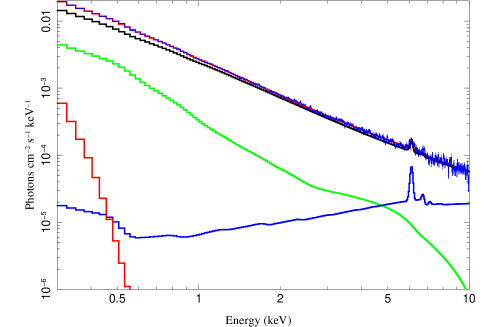
Figure 3: Shows the data and the contributions of the different model components when reflionx was used to model the soft-excess. The data and the best fit model are at the top. The black line just below it shows the powerlaw absorbed by Galactic neutral hydrogen. The green curve shows the contribution of the blurred reflection from an ionised disk (reflionx). The blue curve with narrow emission lines shows the contribution from the PEXMON which is the reflection from a neutral disk. The red curve in the extreme left is the contribution from the disk-blackbody.

The model reflionx (Ross & Fabian, 2005; Crummy et al., 2006) describes the soft-excess as a Compton reflection from an ionised disk. It assumes a semi-infinite slab of optically thick cold gas of constant density, illuminated by a powerlaw producing a reflection component including the fluoresence lines from the ionised species in the gas. We blurred it using kdblur to account for the Doppler and gravitational effects. The full band ($0.3-10\rm\,\,{\rm keV}$) was thus fitted with wabs$\times$xstar$\times$(Gaussian+powerlaw+pexmon+
kdblur(reflionx)). The best fit ionisation parameter is $\rm\xi=493_{-217}^{+116}\rm\,erg\,cm\,s^{-1}$ and the iron abundance with respect to solar is $0.77_{-0.21}^{+0.30}$. The fit statistic was $\,\rm\chi^{2}/dof=271/252$. The narrow emission line modeled using a Gaussian was not required statistically and hence we removed it. We however detected a clear excess in the region $<0.5\rm\,\,{\rm keV}$. The excess could be thermal emission from the thin accretion disk as predicted by Shakura & Sunyaev (1973). We thefore used a disk-blackbody component to model the excess emission, to find that the fit impoved by $\,\Delta\chi^{2}=-8$ to $\,\rm\chi^{2}/dof=263/250$. The F-test significance on addition of this component is $>90\%$ and the fit is acceptable. The best fit temperature of the blackbody is $26_{-4}^{+3}\,{\rm\,eV}$. This temperature nearly conforms with that calculated for the innermost radius of thin disk accreting around a blackhole of mass $\rm M_{BH}\sim 10^{8}\times M_{\odot}$ (Rokaki & Boisson, 1999). The best fit parameter values obtained for this set of models are reported in Table 3, model 1 (column 3). Figure 3 shows the contribution of the various model components in the broad band spectrum.

The optxagnf model, proposed by Done et al. (2012), describes the soft-excess in terms of color-temperature corrected disk emission and Compton upscattering of this disk emission by the low temperature, optically thick inner regions of the disk itself. This model also describes the hard power-law component by thermal Comptonization of disk emission by an optically thin, hot corona external to the disk. In the optxagnf model, the three components – the thermal emission of the disk, cool Comptonization in the optically thick disk, and the hot Comptonization in an optically thin corona, are combined together assuming that they are all ultimately powered by gravitational energy released in the accretion process. We therefore excluded the blackbody and the powerlaw components from our earlier best-fit model when using this model. The parameter $\rm f_{pl}$ determines the fraction of the seed photons that go into producing the hard X-ray powerlaw. We have frozen the norm of optxagnf to one, since the flux is completely calculated by the four parameters: the blackhole mass $\rm M_{BH}$, the spin of the blackhole, the relative accretion rate $\rm L/L_{Edd}$, and the luminosity distance of the source $\rm D_{L}$. We have fixed the value of $\rm log(M_{BH}/M_{\odot})=8.1$ (Rokaki & Boisson, 1999) and $\rm D_{L}$ to $\rm 192\,Mpc$ (obtained from NED). The spin parameter was set to vary. We obtained the best fit relative accretion rate, $\rm log(L/L_{Edd})=-1.361_{-0.004}^{+0.003}$. The spin could not be constrained using this dataset. The full band best fit model stands as $\rm wabs\times xstar\times(optxagnf+pexmon)$. As we had noted that there is no separate powerlaw component, as in previous cases, to which we could tie the PEXMON norm and $\Gamma$, we had followed the following steps. We had fixed the powerlaw contribution of optxagnf model to zero by setting the parameter $\rm f_{PL}=0$ and added a powerlaw model with the model mentioned above. The best fit parameter values of the powerlaw norm and $\Gamma$ thus obtained were noted. We removed the powerlaw from the model and allowed the parameter $\rm f_{PL}$ of optxagnf model free to vary. We fixed the pexmon norm and $\Gamma$ to those obtained using the powerlaw model and carried out our fit.

3.2 The RGS spectral analysis

We fitted the RGS1 and RGS2 spectra simultaneously with the EPIC-pn spectrum for the purpose of testing the presence of warm absorption and emission in the high resolution spectra. We used one of the previously obtained best fit physical models wabs$\times$xstar$\times$(optxagnf+pexmon) for our continuum. The RGS spectra were not grouped and therefore we used the C statistics (Cash, 1979). The best fit value of the statistic for the simultaneous fit was C/dof$=5250/5215$. We checked for the presence of any ionised absorption feature in the RGS data using the XSTAR warm absorber model, but could not find any within $90\%$ statistical significance. This corroborates with our non-detection of a low ionisation warm absorber component in the EPIC-pn spectrum. Earlier studies on the source by Porquet et al. (2004) and Guainazzi (2003) have also not detected any low ionisation warm absorbers. However, we find the presence of an emission feature at $\sim 0.532\rm\,\,{\rm keV}$ (rest-frame) in the EPIC-pn data as well as in the RGS spectra. This emission feature may arise from an ionised cloud intrinsic to the source. We used a Xstar warm emitter additive table model to estimate the cloud parameters which give rise to these features. This table model was created assuming a powerlaw ionising continuum and a turbulent velocity of $200\rm\,\,{\rm km\,s^{-1}}$ for the cloud, and spans the parameter space $-4\leq\log\xi\leq 4$ and $19\leq\log\rm N_{H}\leq 23$. The fit improved by $\Delta C=-36$ to a statistic C/dof$=5214/5211$ on addition of this component. The best fit parameters are: $\log\xi=-1.73_{-0.3}^{+0.4}$, $\rm N_{H}^{WE}=(9.54\pm 0.5)\times 10^{19}\rm\,\,{\rm cm^{-2}}$, $v_{outflow}\sim 12,000\pm 500\rm\,\,{\rm km\,s^{-1}}$. The line was identifed with the neutral Oxygen $K\alpha$ emission line. We also identify one more emission line modeled by the same warm emitter component which corresponds to neutral Neon $K\alpha$ at $\sim 0.85\rm\,\,{\rm keV}$. Figure 4 shows the RGS1 and RGS2 spectra with the best fit model $\rm wabs\times Xstar_{WA}\times(Xstar_{WE}+optxagnf+pexmon)$ when simultaneously fitted with the EPIC-pn data, along with the residuals.

3.3 The Optical Monitor data

From Table 3 we find that both the soft-excess models (reflionx and optxagnf) yield similar fitting statistics to the EPIC-pn data. We further investigated this result by simultaneously fitting the UV data from the optical monitor (OM) telescope and the EPIC-pn data. The OM observed ESO 198–G024 simultaneously with the EPIC-pn with five filters. We used the SAS task omichain to reprocess the OM data. We obtained the flux values from the source list files that were generated by the omichain task. The right ascension and declination of ESO 198–G24 were matched in the combined list and we obtained the source flux at the five wavelengths corresponding to the five filters. The Galactic extinction correction was done following Fitzpatrick (1999) redenning law with $\rm R_{v}=3.1$. The observed flux at $2120\rm\AA$ (UVW2 filter) is $5.23\pm 0.06\times 10^{-15}\rm\,erg\,cm^{-2}\,s^{-1}\AA^{-1}$ and after correcting for the Galactic reddening ($\rm A_{\lambda}=0.282$) we obtained a flux of $6.78\pm 0.07\times 10^{-15}\rm\,erg\,cm^{-2}\,s^{-1}\AA^{-1}$. The Galactic extinction corrected fluxes obtained in the five filters are given in the Table 4.

The measured OM flux at different wavelengths are also affected by the host galaxy contamination, the nuclear emission lines and the intrinsic reddening, which yield a considerable amount of systematic uncertainty in the measured optical-UV continuum flux. Accurate measurements and estimates of these quantities are not known, so we have added a typical $5\%$ systematic error to the OM fluxes. The two sets of models reflionx and optxagnf, were used to jointly fit the OM and EPIC-pn data. The best fit parameter values are quoted in Table 3 (columns 5 and 6). We find that both the models describe the data with similar statistics. The higher values of $\,\rm\chi^{2}/dof$ are due to the small error bars on the OM data points, so even a small deviation from the model yields a poor statistic. Note that the parameters of the models pexmon, Xstar-WA and Gaussian were frozen in the joint fit as they were determined by the EPIC-pn fit only. Figure 5 shows the plot for the two best fit models along with the OM data points.

3.4 The long-term X-ray and UV variability

The joint fit to the OM and the EPIC-pn data from the observation 3 did not prefer any one of the soft-excess models over the other. We then looked for possible variability in the source and its pattern to help distinguish between them. We also performed spectral analysis of observation 1 (2000) and observation 2 (2001) (see Table 1). We fitted the three EPIC-pn ($0.3-10\rm\,\,{\rm keV}$) datasets separately with simple models $\rm wabs*(bbody+powerlaw+pexmon+Gaussian)$. The powerlaw slope and the blackbody temperature for all the three datasets were similar. However the X-ray flux in the $0.3-10\rm\,\,{\rm keV}$ band had varied from observation 2 to 3 (see Figure 6 and Table 5). The EPIC-pn datasets for observations 1 and $2$ were analysed in detail using the two models reflionx and optxagnf for the soft-excess which are reported in Table 6. For observation 1 both models describe the dataset well, but in case of observation 2 the reflionx model gives a statistically better fit ($\,\rm\chi^{2}/dof=229/232$) than the optxagnf ($\,\rm\chi^{2}/dof=253/235$). The continuum model parameters except for the normalisations are similar for the two observations (see Table 4). In the UV band the flux increased by $23\%$ from the observation 2 to observation 3. The first observation used only one filter (U band) which was not used in the second observation. We also find that when the UV flux increased by $23\%$, the X-ray flux decreased by almost the similar fraction ($\sim 20\%$). We have also carried out simultaneous fit of the EPIC-pn and OM datasets for the three observations to obtain better constraints on the parameters for the lower signal to noise data. We found that the parameter values for the two sets of models reflionx and optxagnf are similar to those obtained in individual fits and therefore do not quote them separately. We discuss the implications of these results in the next section.

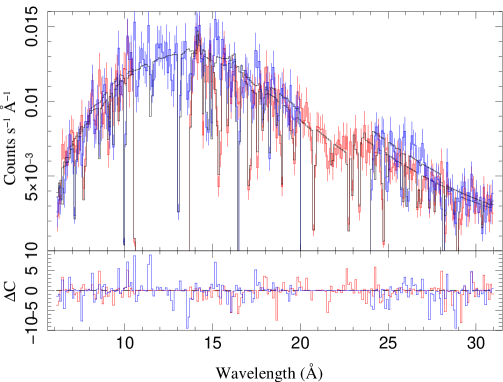
Figure 4: The observed RGS1 and RGS2 spectral data along with the best-fit model (in black) for observation 3. There are no statistically significant warm absorbers. However there are two narrow emission lines of neutral Oxygen and Ne arising from a medium with an ouflow velocity of $\sim 12,000\rm\,\,{\rm km\,s^{-1}}$ at wavelengths $\rm 14.5\AA$ and $\rm 23.4\AA$.

.

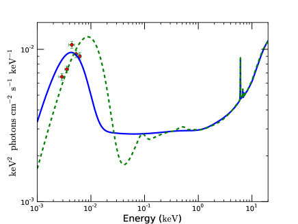
Figure 5: The two sets of best fit models reflionx+diskbb (dashed green) and optxagnf (solid blue) obtained from joint fitting of OM and EPIC-pn data. The OM data points are plotted in red. See section 3.3 for details.

.

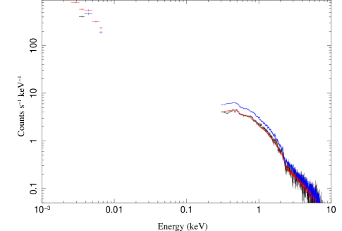
Figure 6: The OM and EPIC-pn data are plotted for the three XMM-Newton observations. The colors black, blue and red stands for the observations 1 , 2 and 3. We see flux variability between the observations in both the EPIC-pn and OM datasets.

.

4 Discussion

The broad band EPIC-pn spectrum of ESO 198–G024 is well described by a soft-excess component, an iron line complex ($6-8\rm\,\,{\rm keV}$), and neutral reflection from distant cold matter. In the iron K band, we detected neutral K$\alpha$, K$\beta$ emission lines and absorption features at energies $>7\rm\,\,{\rm keV}$. The $0.3-10\rm\,\,{\rm keV}$ unabsorbed flux of the source is $2\times 10^{-11}\rm\,erg\,cm^{-2}\,s^{-1}$. The continuum parameters for e.g. powerlaw slope ($\Gamma=1.81\pm 0.01$), black body temperature ($kT=0.08\pm 0.02,\,0.17\pm 0.07\rm\,\,{\rm keV}$) and the neutral reflection coefficient ($R=-1.62\pm 0.1$) are similar to those found in typical Seyfert 1 galaxies (Piconcelli et al., 2005; Winter et al., 2012). Below we discuss our main results.

4.1 The Soft X-ray excess emission

ESO 198–G024 shows a prominent soft X-ray excess emission below $<2\rm\,\,{\rm keV}$ over an absorbed power-law component. The soft excess flux is $\sim 1.00\times 10^{-12}\rm\,erg\,cm^{-2}\,s^{-1}$, which is $\sim 5\%$ of the total $0.3-10\rm\,\,{\rm keV}$ unabsorbed flux. Two blackbodies with temperatures $\rm kT_{BB}=0.08\pm 0.02\rm\,\,{\rm keV}$ and $\rm kT_{BB}=0.17\pm 0.07\rm\,\,{\rm keV}$ yielded satisfactory fit for the soft excess. Thus, the strength and the temperature of the soft excess from ESO 198–G024 are similar to those observed from other Seyfert 1 galaxies. We found no significant warm absorption in the $0.3-2\rm\,\,{\rm keV}$ band. Since the soft-excess was not modified by complex warm absorption, we were able to investigate in detail its possible origin. The temperature of the soft excess when described as thermal emission is much higher than that predicted from an optically thick and geometrically thin accretion disk. To spectrocopically ascertain the possible origin of the soft-excess we modeled it with two physical models – the blurred reflection reflionx and intrinsically Comptonized disk emission optxagnf. Both the models describe the soft-excess statistically well. We discuss below the possible implications of each soft-excess model for ESO  198–G024. The best fit parameter values are quoted in Table 3 columns 3 and 4.

The ionisation parameter of the reflecting disk of the reflionx model is $\xi=493_{-217}^{+116}\rm\,erg\,cm\,s^{-1}$, suggesting a moderate ionisation state. The best fit inner radius $\rm<2.5R_{G}$, and an emissivity index of $4.23_{-0.02}^{+0.50}$ of kdblur clearly indicate that major part of the soft excess flux is emitted from a region very near to the central accreting blackhole. This gives us a picture of an accretion disk which is ionised and reflects the powerlaw continuum incident on it, and most of this reflection comes from within a few gravitational radii. We required an additional disk black body component to model the excess below the energy range $0.5\rm\,\,{\rm keV}$, with a best fit temperature of $\rm kT_{BB}=26_{-4}^{+3}\,{\rm\,eV}$. This points to a dual origin of the soft excess, i.e, the accretion disk acts as a thermal ionised material which emits a blackbody spectrum, and also emits reprocessed fluorescent spectrum. In Fig. 3 we see the individual contribution of each of the continuum and discrete components in the spectra. The reflionx flux in the $0.3-2\rm\,\,{\rm keV}$ band obtained is $2.23\pm 0.06\times 10^{-12}\rm\,erg\,cm^{-2}\,s^{-1}$ and the disk-blackbody flux in the same energy range is $7.76\pm 0.06\times 10^{-14}\rm\,erg\,cm^{-2}\,s^{-1}$. Thus the disk-blackbody component is weak and contributes just $\sim 3.5\%$ of the total soft-excess flux.

The optxagnf describes the soft-excess in terms of the intrinsic thermal emission from the disk and the thermal Comptonization in the disk itself (Done et al., 2012). This model also includes the powerlaw component extending to high energy in the whole band of $0.3-10\rm\,\,{\rm keV}$. The best fit value of the parameter $\rm f_{PL}=0.80\pm 0.02$ points to the fact that $\sim 80\%$ of the power released in the accretion process is converted to powerlaw photons. The best fit value of the temperature of the thermal electrons which Comptonise the seed photons to produce the soft-excess is $\rm kT_{e}=240_{-20}^{+40}\,{\rm\,eV}$ with an optical depth of $15.76$.

In type 1 AGN, the two models reflionx and optxagnf have been claimed to explain the soft X-ray excess. The blurred reflection model naturally explains the similarlity of the soft-excess shape observed across various AGN, the shape does not scale either with the black hole mass or luminosity (Crummy et al., 2006). The reflection model also naturally explains the lag observed between the hard X-ray band dominated by the direct X-ray continuum and the soft X-ray band dominated by the soft excess. The observed lag of about $30{\rm~{}s}$ is interpreted as the reverberation lag between the direct primary continuum and the reflection from the inner disk (Fabian et al., 2009; Emmanoulopoulos et al., 2011). The reflection model also explains the remarkable X-ray spectral variability observed in some AGN where the soft X-ray excess remains nearly constant while the power-law component varies by large factors, see e.g. Fabian et al. (2005).

Dewangan et al. (2007) have investigated the time delay between the emission in the soft and hard X-ray bands for the sources MRK 1044 and AKN 564. They found the soft X-rays leading the hard X-ray band contrary to the expectations from the reflection model but generally consistent with the optically-thick thermal Comptonization model. However, it should be noted that in the reflection model, the soft excess consists of numerous emission lines blended and blurred due to the high velocities and strong gravity in the innermost regions. These lines are usually generated by absorption of continuum photons with energies just above the line energies. The reverberation delay between the continuum and the blurred reflection is expected to be short ($\sim 30{\rm~{}s}$) as observed in some narrow line Seyfert 1 galaxies (Fabian et al., 2009; Emmanoulopoulos et al., 2011). The long time delay $\sim 1700{\rm~{}s}$ reported by Dewangan et al. (2007) could be dominated by the delay due to the Comptonization process. In the optxagnf model of Done et al. (2012), all the soft X-ray excess emission is attributed to the disk. This model is similar to the thermal Comptonization model nthcomp except that it includes the thermal emission from an accretion disk and the inner region of the disk acts like an optically thick Comptonizing corona. Done et al. (2012) have shown that this model describes the soft excess satisfactorily well in the case of extreme narrow-line Seyfert 1 galaxy RE J1034+396, as well as in the low accretion type 1 AGN PG 1048+231. De Marco et al. (2013) have done an extensive study of soft X-ray time lags in AGN. They have found that the time scales of the soft lags are relatively short and are also strongly correlated with the blackhole mass of the AGN, indicating that these lags originate in the inner most regions. Their results best describe the scenario where the delayed soft-excess emission originates from the inner regions of the AGN which is stimulated by a compact central source of hard X-ray photons. ESO 198–G24 is a source in their sample and it has shown a soft time lag of $<2\sigma$ significance. Confirmation of such a time lag would suggest a reflection origin for the SE.

The simultaneously fitted OM and the EPIC-pn data of observation 3 shows both the models reflionx and optxagnf described the datasets equally well. The larger value of $\chi^{2}_{\nu}$ is due to the fact that the OM data points have small errors. From the joint fits using the reflionx+diskbb model we find that the diskblackbody has a much colder temperature of $kT=3.6_{-0.1}^{+0.2}\,{\rm\,eV}$. This is comparable with the inner radius temperature of an accretion disk accreting at a rate of $\rm\log(L_{Bol}/L_{Edd})\sim-1.50$ (obtained using optxagnf model) which is $\sim 6\,{\rm\,eV}$, if we assume an inner most stable radius of six times the Schwarzschild radius $\rm R_{S}$. The best-fit accretion rate obtained using the optxagnf model is comparable to accretion rate $\rm\log(L_{Bol}/L_{Edd})\sim-1.46$ calculated from the broad band $0.001-100\rm\,\,{\rm keV}$ SED. The $0.001-100\rm\,\,{\rm keV}$ bolometric flux calculated from the SED is $1.06\times 10^{-10}\rm\,erg\,cm^{-2}\,s^{-1}$.

We found flux variability both in the UV as well as in the X-rays. The UV fluxes increased from observation 2 to observation 3 by a factor of $23\%$ (UVW2), while the $2-10\rm\,\,{\rm keV}$ flux as well as the soft-excess flux decreased by a factor of $\sim 20\%$. This kind of variability appears to be similar to the X-ray variability observed from black hole X-ray binaries which show a strengthening powerlaw with decreasing disk emission when they make spectral transitions from the high/soft or thermally dominated state to the low/hard states (see e.g., Esin et al., 1997; Belloni et al., 2005). The observed UV and X-ray variability from ESO 198-G24 can possibly be explained in the truncated disk scenario with a spherical corona lying between the truncated radius $\rm R_{in}$ and the inner most stable orbit $\rm R_{ISCO}$. If the inner radius of the truncated disk $R_{in}$ comes closer to the $\rm R_{ISCO}$ , the effective area of the disk will increas leading to an increase in the UV flux while the corona will be compressed and hence the hard X-ray emission will decrease. This is also what we observe when we fit the data for all the three observations using the model reflionx. We find that the best fit inner radius decreases from $\rm R_{in}=4.93_{-1.10}^{+1.12}\,R_{G}$ to $\rm R_{in}<2.5\,R_{G}$ from observation 2 to 3, and we note that the SE flux has also decreased during that time and the UV flux has increased. However it is not clear physically how the inner radius of the truncated disk can be shortened.

The optxagnf model has three distinct emission components– the UV bump, the soft-excess, and the hard X-ray powerlaw, assuming that they are all powered by the gravitational energy released in accretion. The model assumes that the emission thermalises to a blackbody only at a large radius, and at smaller radii the gravitational energy released through accretion is split between powering the soft-excess (optically thick Comptonised disk emission) and the powerlaw (optically thin corona). The flux variability of the source ESO 198–G24 can be possibly explained with this model if the coronal radius moves nearer to the blackhole. In such a scenario the UV emission will increase with a decrease in powerlaw as well as the soft-excess. However, it is not clear physically how the coronal radius can be shortened.

4.2 The Fe line complex and the neutral reflector

In ESO 198–G024, the Fe K$\alpha$ line is slightly broader than the instrument resolution (FWHM velocity $<14000\rm\,\,{\rm km\,s^{-1}}$). Also there is a weaker but significant Fe K$\beta$ line detected at $7.05\rm\,\,{\rm keV}$ rest wavelength. However there is no statistically compelling broad Fe K feature at $\sim 6\rm\,\,{\rm keV}$, clearly indicating that the lines arise from a distant region from the central blackhole. Also the best fit line energy of the Fe K$\alpha$ is $6.41_{-0.05}^{+0.04}\rm\,\,{\rm keV}$ which indicates that the fluorescent line is emitted from a relatively neutral medium. The neutral reflection model PEXMON could describe the Fe K emission lines consistently with the reflected continuum. The reflection coefficient of $\rm R=-1.62_{-0.12}^{+0.10}$ points to an origin from a reflector with a complicated geometry. A reflection coefficient of value 1 would imply a reflector which subtends a solid angle of $2\pi$ at the powerlaw emitter, which is assumed to be isotropically emitting. So in the case of ESO 198–G024 either the emitter is not isotropically illuminating the neutral medium, which may be the torus, or the geometry of the reflecting medium is more complicated. Such values of reflection parameters are not uncommon (Nandra et al., 2007), and in such cases a more complicated geometry is assumed. The best fit Fe abundance is $0.20\pm 0.04$ with respect to solar, for the neutral reflector.

As we noted earlier, the soft-excess of ESO 198–G024 could also be described by a relativistically blurred reflection model. This hints at the possiblity of detecting a broad Fe emission line. However, we do not detect one, which possibly means that the line is blurred beyond detection.

4.3 The high ionisation absorbers

A highly ionised high velocity warm absorber has been tentatively detected in the energy range $>7\rm\,\,{\rm keV}$ at $<2\sigma$ significance. The best fit ionisation parameter is $\xi\sim 1000\rm\,erg\,cm\,s^{-1}$ points to the fact that these features are mainly from FeXXV and/or FeXXVI K-shell resonance absorption having large column densities (Cappi, 2006). We have detected an absorption column of $5\times 10^{21}\rm\,\,{\rm cm^{-2}}$. These outflows are possibly connected with the accretion disk winds, since detailed studies of accretion disk winds by King & Pounds (2003) and Proga & Kallman (2004) suggested that the inner regions of the outflowing material can be highly ionised by the intense radiation and can have large outflow velocities. Since this gas is highly ionised we do not expect it to show any signature in the soft X-ray where the signal to noise is better. The signatures of these features are only found for energies $>7\rm\,\,{\rm keV}$ where the SNR is not very good, hence the detections are usually weak.

5 Conclusion

We have performed a detailed analysis of a long XMM-Newton observation of ESO198–G24. The main results are summarised below:

1. The $0.3-10\rm\,\,{\rm keV}$ continuum is well described by a powerlaw of slope $\Gamma=1.82$, a soft excess component, and a neutral reflection component including FeK emission lines.

2. The soft excess is well described statistically by two physical models, reflionx and optxagnf. It may either arise from a combined effect of the reflection from an ionised disk which is heavily blurred due to gravitational effects, and a thermal emission from a thin accretion disk, described by reflionx. It may also arise from Compton upscattering from an optically thick thermal plasma of temperature $kT_{e}=0.24\rm\,\,{\rm keV}$, described by optxagnf. Jointly fitting the OM and EPIC-pn data we found that both the models yield similar fit statistics and hence cannot be favored one over the other.

3. Variability found in the observations 1, 2 and 3 of the source show that the soft-excess flux decreases when the UV flux increases by the similar amount. This observation can be described in the reflionx scenario by a truncated accretion disk whose inner most radius has come closer to the blackhole leading to an increase in the UV flux and subsequently compressing the corona leading to reduction of the powerlaw flux and therefore soft-excess flux. We find that the best-fit inner radius of the accretion disk decreases from $\rm R_{in}=4.93_{-1.10}^{+1.12}R_{G}$ to $\rm R_{in}<2.5R_{G}$ from observation 2 to 3. Possibly the reflionx+diskbb model describes the soft-excess better for the source ESO 198–G024.

4. We detected the presence of an FeK$\alpha$ line with $\rm v_{FWHM}<14000\rm\,\,{\rm km\,s^{-1}}$. We also detected a narrow FeK$\beta$ line. These lines can arise from the torus or inner BLR. We do not detect any broad Fe line component.

5. A neutral reflection component was detected, which also consistently modeled the FeK$\alpha$ line suggesting a common origin for both.

6. A high ionisation and high velocity warm absorber was tentatively detected at $<2\sigma$ significance. We do not find any evidence for a low ionisation warm absorber.

7. We detect a weak warm emission component with two prominent lines identified as neutral O K$\alpha$ and neutral Ne K$\alpha$.

$Acknowledgements:$ This work is based on observations obtained with XMM-Newton, an ESA science mission with instruments and contributions directly funded by ESA Member States and NASA. Authors are grateful to the anonymous referee for his/her comments which improved the quality of the manusript. Author SL is grateful to CSIR, Govt of India, for supporting this work.

Table 2: The best fit model parameters, using the basic set of models wabs*(bbody+bbody+PEXRAV+egauss+egaus-egaus).

Model	parameters	Values	Comments/ $\,\Delta\chi^{2}$ improvement
wabs	$\rm N_{H}$ (fixed)	$3\times 10^{20}\rm\,\,{\rm cm^{-2}}$
bbody	norm	$4.79_{-0.18}^{+0.20}\times 10^{-5}$
	$\rm kT_{e}$	$0.08\pm 0.02\rm\,\,{\rm keV}$
bbody 2	norm	$1.13_{-0.30}^{+0.20}\times 10^{-5}$	$\,\Delta\chi^{2}=-1424$
	$\rm kT_{e}$	$0.17\pm 0.07\rm\,\,{\rm keV}$	(for the two bbody components)
PEXRAV	norm	$0.0028\pm 0.00002$	$\,\Delta\chi^{2}=-118$
	$\Gamma$	$1.82\pm 0.02$
	rel reflection a	$2.27_{-0.51}^{+0.71}$
	Fe abundance	$0.58_{-0.20}^{+0.40}$
	inclination	60	pegged at this value (cos$(\theta)=0.5$).
Gaussian1	norm b	$9.65_{-2.00}^{+1.50}\times 10^{-6}$	$\,\Delta\chi^{2}=-79$
	Line E	$6.41\pm 0.05$
	$\sigma$	$0.08_{-0.04}^{+0.05}$
Gaussian2	norm c	$2.7_{-1.20}^{+1.10}\times 10^{-6}$	$\,\Delta\chi^{2}=-17$
	Line E	$7.05\pm 0.05$
Gaussian3	norm d	$2.0\pm 1.30\times 10^{-6}$	$\,\Delta\chi^{2}=-7$
	Line E	$7.45_{-0.07}^{+0.07}$
$\rm\chi^{2}/dof$	$264/250\sim 1.04$

^aDue to small band pass of XMM in hard X-ray, the relative reflection parameter could not be estimated properly.
^bWe have used a broad Gaussian to fit the FeK$\alpha$ emission feature..
^cThis is a narrow Gaussian which modeled the FeK$\beta$ emission feature .
^dThis Gaussian modeled the FeK absorption feature.

Table 3: The best fit parameters when the Soft-excess was modeled using physical models for the observation 3, using EPIC-pn dataset as well as EPIC-pn and OM combined datasets.

		EPIC-pn		EPIC-pn+OMa
Model	parameters	Model 1c	Model 2c	Model 1 c	Model 2c
components
wabs	$\rm N_{H}\,(\rm\,\,{\rm cm^{-2}})$	$3\times 10^{20}(f)$	$3\times 10^{20}(f)$	$3\times 10^{20}(f)$	$3\times 10^{20}(f)$
	(frozen)
Warm absorber	$N^{\rm WA}_{\rm H}(\rm\,\,{\rm cm^{-2}})$	$<10^{22}$	$4.87_{-5.30}^{+4.02}\times 10^{21}$	$10^{21}(f)$	$4.87\times 10^{21}(f)$
(XSTAR)	$\rm log(\xi)$	$2.77_{-0.21}^{+0.20}$	$2.92_{-0.12}^{+0.10}$	$2.77(f)$	$2.92(f)$
	redshift b	$-0.057_{-0.005}^{+0.01}$	$-0.057_{-0.005}^{+0.01}$	$-0.057(f)$	$-0.057(f)$
disk-bbody	norm	$1.29^{+50}_{-0.5}\times 10^{7}$	—	$8.9_{-0.4}^{+1.1}\times 10^{9}$
	$\rm kT_{BB}\,(\rm\,\,{\rm keV})$	$0.026_{-0.004}^{+0.003}$	—	$0.0036_{-0.0001}^{+0.0002}$
powerlaw	norm	$0.00258\pm 0.0002$	—	$0.00258(f)$
	$\Gamma$	$1.84_{-0.03}^{+0.02}$	—	$1.84(f)$
PEXMON	norm	$0.00258$	$0.00271$	$0.00258(f)$	$0.00271(f)$
	$\Gamma$	$1.84$	$1.82$	$1.84(f)$	$1.82(f)$
	rel reflection(R)	$-1.62_{-0.12}^{+0.10}$	$-1.43_{-0.20}^{+0.15}$	$-1.62(f)$	$-1.43(f)$
	Fe abundance	$0.20\pm 0.04$	$0.24\pm 0.02$	$0.20(f)$	$0.24(f)$
	inclination (degrees)	$<60$	$<60$	$0(f)$	$0(f)$
Gaussian	norm		$4.64_{+2.0}^{-2.8}\times 10^{-5}$		$4.42\times 10^{-5}(f)$
	Line E (rest)$\rm\,\,{\rm keV}$		$0.533\pm 0.007$		$0.533(f)$
	$\sigma(\,{\rm\,eV})$		$0.001\rm\,\,{\rm keV}(f)$		$0.001\rm\,\,{\rm keV}(f)$
Reflionx	norm	$4.48_{-0.08}^{+1.50}\times 10^{-8}$	—	$7.24_{-1.66}^{+1.70}\times 10^{-8}$
	Fe/solar	$0.77_{-0.21}^{+0.30}$	—	$0.82_{-0.20}^{+0.30}$
	$\Gamma$	$1.84$	—	$1.84$
	$\xi$	$493_{-217}^{+116}$	—	$374_{-95}^{+230}$
Kdblur	index	$2.56_{-0.61}^{+2.51}$	—	$4.23_{-0.21}^{+0.51}$
	$\rm R_{in}\,(r_{g})$	${<2.5}$	—	${<2.5}$
	inclination (degrees)	$<27$	—	$<27$
optxagnf	norm	—	$1$	—	$1$
	$\rm log(L/L_{Edd})$	—	$-1.36_{-0.004}^{+0.003}$	—	$-1.51_{-0.004}^{+0.003}$
	$\rm kT_{e}$	—	$0.24^{+0.04}_{-0.02}$	—	$0.19^{+0.04}_{-0.02}$
	$\tau$	—	$15.76\pm 2$	—	$19.61\pm 3$
	$\Gamma$	—	$1.82\pm 0.01$	—	$1.83\pm 0.03$
	$\rm f_{pl}$	—	$0.80\pm 0.02$	—	$0.842\pm 0.022$
	$\rm r_{cor}\,(r_{g})$	—	$30\pm 12$	—	$72\pm 22$
	$\rm Spin$	—	$<0.99$	—	$<0.99$
$\rm\chi^{2}/dof$		$263/250$	$260/250$	$306/263$	$316/264$

^a$(f)$ stands for frozen parameters. These parameters were constrained by EPIC-pn fit only.
^bRedshift as noted in the observer frame. Negative implies a blue-shift
^cModel 1= $\rm\tt wabs\times Xstar_{WA}\times(diskbb+powerlaw+pexmon+kdblur(reflionx))$; Model 2 =$\rm\tt wabs\times Xstar_{WA}\times(optxagnf+pexmon)$

Table 4: The Optical Monitor data for the three observations.

Filters	Wavelengths	Galactic	Corrected Flux ($\rm f_{\lambda}$)	Corrected Flux ($\rm f_{\lambda}$)	Corrected Flux($\rm f_{\lambda}$)
	(central)	extinction	$\rm\times 10^{-15}\rm\,erg\,cm^{-2}\,s^{-1}\AA^{-1}$	$\rm\times 10^{-15}\rm\,erg\,cm^{-2}\,s^{-1}\AA^{-1}$	$\rm\times 10^{-15}\rm\,erg\,cm^{-2}\,s^{-1}\AA^{-1}$
used	$\rm\AA$	magnitude	(observation-1)	(observation-2)	(observation-3)
UVW2	2120	0.282	—	$5.51\pm 0.08$	$6.78\pm 0.07$
UVM2	2310	0.256	—	—	$6.44\pm 0.043$
UVW1	2910	0.170	—	$4.78\pm 0.006$	$5.64\pm 0.004$
U	3440	0.146	$2.45\pm 0.004$	—	$3.60\pm 0.002$
B	4500	0.116	—	—	$2.29\pm 0.002$

Table 5: The X-ray fluxes of ESO 198–G24 calculated from the EPIC-pn data for the three observations.

observation	observation	$\rm F_{x}(0.3-2)\rm\,\,{\rm keV}$	$\rm F_{x}(2-10)\rm\,\,{\rm keV}$	$\rm F_{x}(0.3-10)\rm\,\,{\rm keV}$	Soft-excess flux
number	id				(bbody)
		$\rm\,erg\,cm^{-2}\,s^{-1}$	$\rm\,erg\,cm^{-2}\,s^{-1}$	$\rm\,erg\,cm^{-2}\,s^{-1}$	$\rm\,erg\,cm^{-2}\,s^{-1}$
1	0112910101	$9.44_{-0.10}^{+0.11}\times 10^{-12}$	$1.07_{-0.03}^{+0.03}\times 10^{-11}$	$2.01_{-0.03}^{+0.03}\times 10^{-11}$	$1.05_{-0.01}^{+0.01}\times 10^{-12}$
2	0067190101	$1.23_{-0.005}^{+0.005}\times 10^{-11}$	$1.29_{-0.01}^{+0.01}\times 10^{-11}$	$2.51_{-0.07}^{+0.04}\times 10^{-11}$	$1.23_{-0.005}^{+0.008}\times 10^{-12}$
3	0305370101	$9.18_{-0.02}^{+0.04}\times 10^{-12}$	$1.086_{-0.01}^{+0.009}\times 10^{-11}$	$2.00_{-0.02}^{+0.01}\times 10^{-11}$	$1.00_{-0.01}^{+0.008}\times 10^{-12}$

—————————————————–

Table 6: The best fit parameters when we modeled the EPIC-pn and OM datasets of observations 1 and 2.

		Observation 1		Observation 2
Model	paramters	Model 1c	Model 2c	Model 1c	Model 2c
components
wabs	$\rm N_{H}\,(\rm\,\,{\rm cm^{-2}})$	$3\times 10^{20}$	$3\times 10^{20}$	$3\times 10^{20}$	$3\times 10^{20}$
	(fixed)
disk-bbody	norm	$>2\times 10^{7}$	—	$>3\times 10^{9}$
	$\rm kT_{BB}\,(\rm\,\,{\rm keV})$	$0.025_{-0.019}^{+0.001}$	—	$0.003_{-0.001}^{+0.001}$
powerlaw	norm	$0.00266^{+0.00003}_{-0.0015}$	—	$0.0032\pm 0.0002$	—
	$\Gamma$	$1.82_{-0.41}^{+0.08}$	—	$1.86\pm 0.04$	—
PEXMON	norm	$0.00266$	$0.0027$	$0.0032$	$0.0032$
	$\Gamma$	$1.82$	$1.82$	$1.86$	$1.85$
	rel reflection	$-0.81_{-0.65}^{+0.60}$	$-0.64_{-0.2}^{+0.55}$	$-0.85_{-0.21}^{+0.37}$	$-0.687_{-0.391}^{+0.372}$
	Fe abundance	$0.16_{-0.37}^{+0.5}$	$0.88\pm 0.5$	$0.38_{-0.22}^{+0.40}$	$0.60_{-0.18}^{+0.40}$
	inclination (degrees)	$<60$	$<60$	$<60$	$<60$
Reflionx	norm	$7.6_{-3.5}^{+3}\times 10^{-9}$	—	$5.22_{-0.88}^{+1.66}\times 10^{-8}$	—
	Fe/solar	$<20$	—	$0.50_{+0.21}^{-0.20}$	—
	$\Gamma$	$1.82$	—	$1.86$	—
	$\xi$	$<10000$	—	$971_{-210}^{+400}$	—
Kdblur	index	$4.23_{-2.10}^{+2.20}$	—	$4.8_{-1.0}^{+3.5}$	—
	$\rm R_{in}\,(r_{g})$	${<4.5}$	—	$4.93_{-1.10}^{+1.12}$	—
	inclination	$<60$degrees		$<60$degrees	—
optxagnf	norm	—	$1$	—	$1$
	$\rm log(L/L_{EDD})$	—	$-1.42_{-0.21}^{+0.55}$	—	$-1.44_{-0.05}^{+0.05}$
	$\rm kT_{e}$	—	$0.21^{+0.04}_{-0.02}$	—	$0.20^{+0.04}_{-0.02}$
	$\tau$	—	$20.63\pm 3$	—	$19.68\pm 2$
	$\Gamma$	—	$1.79_{-0.03}^{+0.07}$	—	$1.85_{-0.04}^{+0.07}$
	$\rm f_{pl}$	—	$0.89\pm 0.02$	—	$0.851\pm 0.101$
	$\rm r_{cor}\,(r_{g})$	—	$<100$	—	$65_{-21}^{+55}$
	$\rm Spin$	—	$<0.99$	—	$<0.76$
$\rm\chi^{2}/dof$		$163/183$	$164/183$	$243/232$	$253/232$

^cModel 1= $\rm\tt wabs\times(powerlaw+pexmon+kdblur(reflionx))$; Model 2 =$\rm\tt wabs\times(optxagnf+pexmon)$

References

- Arnaud et al. (1985) Arnaud K. A., Branduardi-Raymont G., Culhane J. L., Fabian A. C., Hazard C., McGlynn T. A., Shafer R. A., Tennant A. F., Ward M. J., 1985, MNRAS, 217, 105
- Belloni et al. (2005) Belloni T., Homan J., Casella P., van der Klis M., Nespoli E., Lewin W. H. G., Miller J. M., Méndez M., 2005, A&A, 440, 207
- Braito et al. (2007) Braito V., Reeves J. N., Dewangan G. C., George I., Griffiths R. E., Markowitz A., Nandra K., Porquet D., Ptak A., Turner T. J., Yaqoob T., Weaver K., 2007, ApJ, 670, 978
- Cappi (2006) Cappi M., 2006, Astronomische Nachrichten, 327, 1012
- Cash (1979) Cash W., 1979, ApJ, 228, 939
- Chartas et al. (2003) Chartas G., Brandt W. N., Gallagher S. C., 2003, ApJ, 595, 85
- Crummy et al. (2006) Crummy J., Fabian A. C., Gallo L., Ross R. R., 2006, MNRAS, 365, 1067
- de Marco et al. (2009) de Marco B., Iwasawa K., Cappi M., Dadina M., Tombesi F., Ponti G., Celotti A., Miniutti G., 2009, A&A, 507, 159
- De Marco et al. (2013) De Marco B., Ponti G., Cappi M., Dadina M., Uttley P., Cackett E. M., Fabian A. C., Miniutti G., 2013, MNRAS, 431, 2441
- Dewangan et al. (2007) Dewangan G. C., Griffiths R. E., Dasgupta S., Rao A. R., 2007, ApJ, 671, 1284
- Done et al. (2012) Done C., Davis S. W., Jin C., Blaes O., Ward M., 2012, MNRAS, 420, 1848
- Emmanoulopoulos et al. (2011) Emmanoulopoulos D., McHardy I. M., Papadakis I. E., 2011, MNRAS, 416, L94
- Esin et al. (1997) Esin A. A., McClintock J. E., Narayan R., 1997, ApJ, 489, 865
- Fabian et al. (2002) Fabian A. C., Crawford C. S., Iwasawa K., 2002, MNRAS, 331, L57
- Fabian et al. (2005) Fabian A. C., Miniutti G., Iwasawa K., Ross R. R., 2005, MNRAS, 361, 795
- Fabian et al. (2009) Fabian A. C., Zoghbi A., Ross R. R., Uttley P., Gallo L. C., Brandt W. N., Blustin A. J., Boller T., Caballero-Garcia M. D., Larsson J., Miller J. M., Miniutti G., Ponti G., Reis R. C., Reynolds C. S., Tanaka Y., Young A. J., 2009, Nat, 459, 540
- Fitzpatrick (1999) Fitzpatrick E. L., 1999, PASP, 111, 63
- Gierliński & Done (2004) Gierliński M., Done C., 2004, MNRAS, 349, L7
- Gierliński & Done (2006) Gierliński M., Done C., 2006, MNRAS, 371, L16
- Guainazzi (2003) Guainazzi M., 2003, A&A, 401, 903
- Houck & Denicola (2000) Houck J. C., Denicola L. A., 2000, in Manset N., Veillet C., Crabtree D., eds, Astronomical Data Analysis Software and Systems IX Vol. 216 of Astronomical Society of the Pacific Conference Series, ISIS: An Interactive Spectral Interpretation System for High Resolution X-Ray Spectroscopy. p. 591
- Kalberla et al. (2005) Kalberla P. M. W., Burton W. B., Hartmann D., Arnal E. M., Bajaja E., Morras R., Pöppel W. G. L., 2005, A&A, 440, 775
- Kallman et al. (2004) Kallman T. R., Palmeri P., Bautista M. A., Mendoza C., Krolik J. H., 2004, ApJS, 155, 675
- King & Pounds (2003) King A. R., Pounds K. A., 2003, MNRAS, 345, 657
- Laor (1991) Laor A., 1991, ApJ, 376, 90
- Magdziarz et al. (1998) Magdziarz P., Blaes O. M., Zdziarski A. A., Johnson W. N., Smith D. A., 1998, MNRAS, 301, 179
- Magdziarz & Zdziarski (1995) Magdziarz P., Zdziarski A. A., 1995, MNRAS, 273, 837
- Nandra et al. (2007) Nandra K., O’Neill P. M., George I. M., Reeves J. N., 2007, MNRAS, 382, 194
- Piconcelli et al. (2005) Piconcelli E., Jimenez-Bailón E., Guainazzi M., Schartel N., Rodríguez-Pascual P. M., Santos-Lleó M., 2005, A&A, 432, 15
- Porquet et al. (2004) Porquet D., Kaastra J. S., Page K. L., O’Brien P. T., Ward M. J., Dubau J., 2004, A&A, 413, 913
- Porquet et al. (2004) Porquet D., Reeves J. N., O’Brien P., Brinkmann W., 2004, A&A, 422, 85
- Pounds et al. (2003) Pounds K. A., King A. R., Page K. L., O’Brien P. T., 2003, MNRAS, 346, 1025
- Pravdo et al. (1981) Pravdo S. H., Nugent J. J., Nousek J. A., Jensen K., Wilson A. S., Becker R. H., 1981, ApJ, 251, 501
- Proga & Kallman (2004) Proga D., Kallman T. R., 2004, ApJ, 616, 688
- Rokaki & Boisson (1999) Rokaki E., Boisson C., 1999, MNRAS, 307, 41
- Ross & Fabian (2005) Ross R. R., Fabian A. C., 2005, MNRAS, 358, 211
- Shakura & Sunyaev (1973) Shakura N. I., Sunyaev R. A., 1973, A&A, 24, 337
- Shu et al. (2010) Shu X. W., Yaqoob T., Wang J. X., 2010, ApJS, 187, 581
- Singh et al. (1985) Singh K. P., Garmire G. P., Nousek J., 1985, ApJ, 297, 633
- Tombesi et al. (2010) Tombesi F., Cappi M., Reeves J. N., Palumbo G. G. C., Yaqoob T., Braito V., Dadina M., 2010, A&A, 521, A57
- Turner et al. (1993) Turner T. J., George I. M., Mushotzky R. F., 1993, ApJ, 412, 72
- Winter et al. (2012) Winter L. M., Veilleux S., McKernan B., Kallman T. R., 2012, ApJ, 745, 107