A nonlocal kinetic energy functional for an inhomogeneous two-dimensional Fermi gas

Abstract

The average-density approximation is used to construct a nonlocal kinetic energy functional for an inhomogeneous two-dimensional Fermi gas. This functional is then used to formulate a Thomas-Fermi von Weizsäcker-like theory for the description of the ground state properties of the system. The quality of the kinetic energy functional is tested by performing a fully self-consistent calculation for an ideal, harmonically confined, two-dimensional system. Good agreement with exact results are found, with the number and kinetic energy densities exhibiting oscillatory structure associated with the nonlocality of the energy functional. Most importantly, this functional shows a marked improvement over the two-dimensional Thomas-Fermi von Weizsäcker theory, particularly in the vicinity of the classically forbidden region.

I Introduction

One of the central ingredients in the density-functional theory (DFT) description DFT of an interacting many-body Fermi system is the kinetic energy (KE). In the Kohn-Sham (KS) scheme KS , the kinetic energy functional is defined to be that of a system of noninteracting particles having the same ground state density as the interacting system. Formally, the KS energy functional is,

$$E[\rho]=T[\rho]+E_{\rm int}[\rho]+\int d^{3}r~{}v_{\rm ext}({\bf r})\rho({\bf r})~{},$$ (1)

where $E_{\rm int}[\rho]$ accounts for interactions and $v_{\rm ext}({\bf r})$ is some externally imposed potential. By its definition, the KS kinetic energy functional $T[\rho]$ of $N$-independent particles is

$$T[\rho]=\sum_{i=1}^{N}\int d^{3}r~{}\phi_{i}^{\star}({\bf r})\left(-\frac{\hbar^{2}}{2m}\nabla^{2}\right)\phi_{i}({\bf r})~{}.$$ (2)

The $\phi_{i}({\bf r})$ are single-particle orbitals, each satisfying a Schrödingier-like equation arising from the variational minimization of Eq. (1), viz.,

$$-\frac{\hbar^{2}}{2m}\nabla^{2}\phi_{i}({\bf r})+v_{\rm eff}({\bf r})\phi_{i}({\bf r})=\varepsilon_{i}\phi_{i}({\bf r})~{},~{}~{}~{}~{}i=1,...,N$$ (3)

with the effective potential given by

$$v_{\rm eff}({\bf r})\equiv\frac{\delta E_{\rm int}[\rho]}{\delta\rho({\bf r})}+v_{\rm ext}({\bf r})~{}.$$ (4)

The ground state density is obtained from

$$\rho({\bf r})=\sum_{i=1}^{N}\phi_{i}^{\star}({\bf r})\phi_{i}({\bf r})~{},$$ (5)

subject to the normalization constraint

$$N=\int d^{3}r~{}\rho({\bf r})~{}.$$ (6)

The implementation of the KS scheme requires some approximation to be made for the generally unknown interaction functional, $E_{\rm int}[\rho]$. Although the KE is treated exactly, it suffers from having to solve $N$ self-consistent equations, Eq. (3), which can be numerically expensive.

Rather than determining the KE via the KS approach, an alternative method is to construct an explicit KE density functional, $T[\rho]$, thereby avoiding the additional computational task of determining the KS orbitals. This is the so-called orbital-free DFT, and captures the original spirit of DFT whereby one focuses exclusively on the density. Since the noninteracting KE of an arbitrary inhomogeneous system is not generally known as an explicit functional of the density, approximations must be made for its construction.

The most primitive functional is that provided by the local-density approximation (LDA), in which the KE density is approximated by that of a uniform system DFT . The LDA is expected to work for systems with slow spatial variations and can be improved by including gradient corrections which take spatial inhomogeneities explicitly into account. In three-dimensions (3D), gradient corrections can be obtained systematically from either a linear response DFT ; HK , or a semiclassical gradient expansion approach brack_bhaduri ; wigner ; kirkwood ; kirzhnits57 ; jennings76 . In particular, the leading order functional series for the 3D noninteracting KE functional, using either approach, is given by (in what follows, a spin degeneracy factor of two is always assumed)

$$T[\rho]=C_{3}\int d^{3}r\rho^{5/3}({\bf r})+\frac{1}{9}\frac{\hbar^{2}}{8m}\int d^{3}r\frac{|\nabla\rho({\bf r})|^{2}}{\rho({\bf r})}~{},$$ (7)

where $C_{3}=3(3\pi^{2})^{2/3}\hbar^{2}/10m$. The first term represents the Thomas-Fermi (TF) KE functional for a uniform system (i.e., the LDA) while the second term is $1/9$ the original von Weizsäcker (vW) functional vW . Equation (7) is exact up to ${\cal O}(k^{2})$ in linear response ($k/2k_{F}\ll 1$, where $k_{F}$ is the 3D Fermi wave number), but works quite well even for strongly inhomogeneous systems. Higher order terms involving gradients of the density may be added to Eq. (7), but such terms are not guaranteed to improve the quality of the KE functional, and in some circumstances, may actually diverge DFT ; hodges73 .

In applications, the functional

$$T[\rho]=C_{3}\int d^{3}r\rho^{5/3}({\bf r})+\lambda_{\rm vW}\frac{\hbar^{2}}{8m}\int d^{3}r\frac{|\nabla\rho({\bf r})|^{2}}{\rho({\bf r})}~{}$$ (8)

is often used, where $\lambda_{\rm vW}$ (the vW coefficient) is an adjustable parameter. The total energy in this approximation is then given by the Thomas-Fermi von Weizsäcker (TFvW) functional

$$E[\rho]=C_{3}\int d^{3}r\rho^{5/3}({\bf r})+\lambda_{\rm vW}\frac{\hbar^{2}}{8m}\int d^{3}r\frac{|\nabla\rho({\bf r})|^{2}}{\rho({\bf r})}+E_{\rm int}[\rho]+\int d^{3}r~{}v_{\rm ext}({\bf r})\rho({\bf r})~{}.$$ (9)

The parameter $\lambda_{\rm vW}$ can be tuned to obtain the best agreement with the energy generated by a KS orbital calculation.

The minimization of Eq. (9) with respect to the density, $\rho({\bf r})$, for a fixed number of particles, leads to a single Schrödinger-like equation for the vW wave function, $\psi({\bf r})\equiv\sqrt{\rho({\bf r})}$,

$$-\lambda_{\rm vW}\frac{\hbar^{2}}{2m}\nabla^{2}\psi({\bf r})+v_{\rm eff}({\bf r})\psi({\bf r})=\mu\psi({\bf r})$$ (10)

where the effective one-body potential is given by

$$v_{\rm eff}({\bf r})=\frac{5}{3}C_{3}\rho^{2/3}({\bf r})+\frac{\delta E_{\rm int}[\rho]}{\delta\rho({\bf r})}+v_{\rm ext}({\bf r})~{}.$$ (11)

The vW term, $-(\lambda_{\rm vW}\hbar^{2}/2m)\nabla^{2}\psi({\bf r})$, is known to provide a smooth decay of the spatial density into the classically forbidden region, and cures the unphysical, sharp cutoff of the density at the classical turning point found within the TF approximation brack_bhaduri . This approach is easy to implement and computationally inexpensive (i.e., only a single self-consistent equation, Eq. (10), needs to be solved). For 3D Coulombic systems with local exchange, it is referred to as the Thomas-Fermi-Dirac-von Weiszäcker (TFDW) theory and has yielded good results in various applications chizmeshya88 ; zaremba_tso .

For the inhomogeneous two-dimensional (2D) Fermi gas, it is natural to try to follow the same formulation as the 3D TFvW theory outlined above. Unfortunately, in 2D, it is known that neither the linear response HK , or semiclassical methods geldhart86 ; holas91 ; salasnich ; koivisto ; PhD ; putaja ; vanzyl11 yield any gradient corrections whatsoever. This is troublesome, since we know that the LDA cannot be exact for an inhomogenous system. Nevertheless, gradient corrections introduced in an ad hoc fashion do provide a more realistic description of 2D density distributions. Specifically, the 2D analogue of Eq. (8) reads

$$T[\rho]=C_{2}\int d^{2}r~{}\rho^{2}({\bf r})+\lambda_{\rm vW}\frac{\hbar^{2}}{8m}\int d^{2}r\frac{|\nabla\rho({\bf r})|^{2}}{\rho({\bf r})}~{},$$ (12)

where $C_{2}=\pi\hbar^{2}/2m$. Equation (12) has been used to construct the 2D version of the TFDW theory for an inhomogeneous two-dimensional electron gas (2DEG) zaremba_tso ; PhD , and more recently, to describe the equilibrium properties of a 2D harmonically trapped, spin polarized dipolar Fermi gas vanzyl_pisarski . Although the vW term cannot be justified on the basis of a gradient expansion, the 2D TFDW theory was nonetheless successful in various applications to 2DEGs vanzyl1 ; vanzyl2 ; vanzyl3 ; vanzyl4 .

In this paper, we make use of the average-density approximation (ADA) to define a nonlocal KE functional, which allows us to systematically treat a spatially inhomogeneous 2D Fermi gas without the use of any ad hoc, e.g., vW, gradient corrections. This functional is then utilized to formulate a self-consistent TFvW-like theory for the 2D inhomogeneous Fermi gas. The efficacy of the theory is tested in Sec. III by comparing our self-consistent calculations for the ground state properties of an ideal, harmonically trapped Fermi gas, with exact results, and with the results of the 2D TFvW theory using an optimal vW coefficient (i.e., the value of $\lambda_{\rm vW}$ for which Eq. (12) yields the exact KE for the TFvW self-consistent density) vanzyl_pisarski . In Sec. IV, we present our closing remarks.

II The average-density approximation

The ADA was first proposed in the late $1970$s by Alonso et al. alonso and Gunnarsson et al. gunnarsson , as a way to go beyond the LDA for calculations of the exchange and correlation energies of non-uniform electron systems. These same ideas were later applied in the construction of nonlocal kinetic energy functionals in 1D herring ; comb97 ; gonzalez98 and 3D chacon85 ; garcia96 ; wang ; chai2007 ; chacon07 ; perrot systems. It is within the latter context that we wish to briefly review the essential ideas behind the ADA. In this section of the paper, we will use atomic units ($\hbar=m=1$).

At the heart of the ADA is the specification of the nonlocal KE functional in terms of an average-density (analogous expressions hold for 1D and 2D), viz.,

$$T_{\rm nl}[\rho({\bf r})]=\int d^{3}r~{}\rho({\bf r})t(\bar{\rho}({\bf r}))~{},$$ (13)

where $t(x)$ is the kinetic energy per particle of the uniform system, and the average density, $\bar{\rho}({\bf r})$, is defined as

$$\bar{\rho}({\bf r})=\int d^{3}r^{\prime}\rho({\bf r}^{\prime})w({\bf r}^{\prime}-{\bf r};\rho({\bf r}))~{}.$$ (14)

The nonlocal character of the inhomogeneous system is then captured by the weight function $w({\bf r};\rho)$, which is normalized according to

$$\int d^{3}x~{}w({\bf x};\rho)=1~{}.$$ (15)

The normalization ensures that Eq. (13) reproduces the exact kinetic energy of a uniform system. The weight function itself is fully specified by also demanding that the second functional derivative of Eq. (13), when evaluated for a uniform system of density, $\rho_{0}$, leads to the exact static linear response function HK , viz.,

$$\mathcal{F}\left[\frac{\delta^{2}T_{\rm nl}[\rho]}{\delta\rho({\bf r})\delta\rho({\bf r}^{\prime})}\right]_{\rho({\bf r})=\rho_{0}}=-\frac{1}{\chi_{0}({\bf k})}~{},$$ (16)

where $\mathcal{F}$ denotes a Fourier transform (FT) from ${\bf r}-{\bf r}^{\prime}$ to ${\bf k}$. Performing the functional derivatives is straightforward, and after taking the FT, we obtain the following general result chacon85

$$\mathcal{F}\left[\frac{\delta^{2}T_{\rm nl}[\rho]}{\delta\rho({\bf r})\delta\rho({\bf r}^{\prime})}\right]_{\rho({\bf r})=\rho_{0}}=2t^{\prime}(\rho_{0})w(k;\rho_{0})+\rho_{0}t^{\prime\prime}(\rho_{0})w(k;\rho_{0})^{2}+2\rho_{0}t^{\prime}(\rho_{0})\frac{dw(k;\rho_{0})}{d\rho_{0}}~{},$$ (17)

where $w(k;\rho_{0})$ is the FT of $w(|{\bf r}-{\bf r}^{\prime}|;\rho_{0})$. In principle, once the weight function is known, Eq. (13) defines a nonlocal KE functional, which will exactly reproduce the KE of the uniform gas, and whose second functional derivative is exact in the uniform limit note_nl . Whether this prescription for the KE functional also provides a good description for an inhomogeneous system must be established separately.

In practice, however, the right-hand side of Eq. (16) is divergent in the $k\to\infty$ limit, and this divergence occurs regardless of dimensionality. This is an undesirable feature, as the weight function will also inherit the divergence. One way to avoid this issue is to remove the offending terms from the right-hand side of Eq. (16), and then solve for a new weight function with no divergent behaviour. The details of this procedure requires an explicit analytical form for $\chi_{0}(k)$, so it is necessary to take up the rest of our discussion in strictly 2D.

II.1 Two-dimensional nonlocal kinetic energy functional

The exact static response function, $\chi_{0}(k)$, for a uniform 2D Fermi gas of density $\rho_{0}$ is given by stern

$$\chi_{0}(\eta)=\begin{cases}-\dfrac{1}{\pi},&\eta<1\\ -\dfrac{1}{\pi}\left(1-\sqrt{1-\dfrac{1}{\eta^{2}}}\right),&\eta\geq 1~{},\end{cases}$$ (18)

with $\eta\equiv k/(2k_{F})$, and $k_{F}=\sqrt{2\pi\rho_{0}}$. This expression is the 2D analogue of the 3D Lindhard function lindhard .

It is useful to write Eq. (18) as

$$-\frac{1}{\chi_{0}(\eta)}=\pi F(\eta)~{},$$ (19)

where

$$F(\eta)=\begin{cases}1,&\eta<1~{},\\ \dfrac{1}{1-\sqrt{1-\dfrac{1}{\eta^{2}}}},&\eta\geq 1~{}.\end{cases}$$ (20)

Note that $F(\eta)$ has a pole at $\eta\to\infty$, and is piecewise continuous at $\eta=1$. Equation (16) then amounts to

$$2t^{\prime}(\rho_{0})w(k;\rho_{0})+\rho_{0}t^{\prime\prime}(\rho_{0})w(k;\rho_{0})^{2}+2\rho_{0}t^{\prime}(\rho_{0})\frac{dw(k;\rho_{0})}{d\rho_{0}}=\pi F(\eta)~{}.$$ (21)

The kinetic energy per particle for the uniform 2D gas is given by

$$t(\rho_{0})=\frac{\pi}{2}\rho_{0}~{},$$ (22)

and we see that Eq. (21) reduces to a first-order ordinary differential equation (ODE). In view of the dependence of the response function on the scaled wavevector $\eta$, we will assume that the weight function has a similar dependence, namely $w(k;\rho_{0})\equiv w(k/2k_{F})=w(\eta)$. As a result,

$$\rho_{0}\frac{dw(k;\rho_{0})}{d\rho_{0}}=-\frac{\eta}{2}w^{\prime}(\eta)~{},$$ (23)

and the ODE for the weight function then reads

$$w(\eta)-\frac{\eta}{2}w^{\prime}(\eta)=F(\eta)~{}.$$ (24)

The normalization condition, Eq. (15), in real space implies that $w(\eta=0)=1$, which is automatically satisfied by the solution of Eq. (24). Once the solution to Eq. (24) is obtained, the nonlocal KE functional is given by

$$T_{\rm nl}[\rho]=\frac{\pi}{2}\int d^{2}r\int d^{2}r^{\prime}~{}\rho({\bf r}^{\prime}){w}({\bf r}-{\bf r}^{\prime};\rho({\bf r})){\rho}({\bf r})~{}.$$ (25)

It is straightforward to show that $w(\eta)$ is given by

$$w(\eta)=-2\eta^{2}\int\frac{F(\eta)}{\eta^{3}}d\eta+c\eta^{2}~{},$$ (26)

where $c\eta^{2}$ is the solution of the homogeneous equation. For $\eta<1$, $F(\eta)=1$, and we obtain

$$w(\eta)=1+c_{1}\eta^{2}~{},$$ (27)

where $c_{1}$ is fixed by demanding continuity of $w(\eta)$ at $\eta=1$. For $\eta\geq 1$, we have

$$w(\eta) = -2\eta^{2}\int_{1}^{\eta}\frac{1}{t^{3}}\frac{1}{1-\sqrt{1-1/t^{2}}}dt+c_{2}\eta^{2}$$ (28)

$$= -4\eta^{2}\ln\eta+2\eta\sqrt{\eta^{2}-1}-2\eta^{2}\ln\left[1+\sqrt{1-\frac{1}{\eta^{2}}}\right]+c_{2}\eta^{2}~{}.$$

In the $\eta\to\infty$ limit, Eq. (28) has the following behaviour

$$w(\eta)\sim-4\eta^{2}\ln\eta+2\eta^{2}-\ln 4\eta^{2}+c_{2}\eta^{2}-\frac{1}{2}\cdots~{}.$$ (29)

The $\eta^{2}$ divergence in Eq. (29) can be eliminated by choosing $c_{2}=\ln 4-2$, but as discussed above, $w(\eta)$ still has a rather nasty divergence $-4\eta^{2}\ln\eta$ for $\eta\to\infty$. The origin of this divergence can be traced back to the $\eta\to\infty$ behaviour of $F(\eta)$, namely

$$F(\eta)\sim 2\eta^{2}~{}.$$ (30)

Therefore, deleting the $\eta\to\infty$ terms from $F(\eta)$ will yield a new weight function with no divergent behaviour, viz.,

$$w_{0}(\eta)-\frac{\eta}{2}w_{0}^{\prime}(\eta)=F(\eta)-2\eta^{2}~{}.$$ (31)

Note that here, $w_{0}(0)=1$, so the normalization of the weight function is preserved. The solution to Eq. (31) is given by

$$w_{0}(\eta) = \left[{4\eta^{2}\ln\eta}+1+\left(\ln 4-3\right)\eta^{2}\right]\Theta(1-\eta)$$ (32)

$$+ \left[2\eta\sqrt{\eta^{2}-1}+\eta^{2}(\ln 4-2)-2\eta^{2}\ln\left(1+\sqrt{1-\frac{1}{\eta^{2}}}\right)\right]\Theta(\eta-1)~{},$$

which no longer exhibits any divergences.

In order to satisfy Eq. (21), however, we must now write the nonlocal KE functional as

$$T_{\rm nl}[\rho]=\frac{\pi}{2}\int d^{2}r\int d^{2}r^{\prime}~{}\rho({\bf r}^{\prime}){w_{0}}({\bf r}-{\bf r}^{\prime};\rho({\bf r})){\rho}({\bf r})+T_{\rm vW}[\rho]~{},$$ (33)

where

$$T_{\rm vW}[\rho]=\frac{1}{8}\int d^{2}r\frac{|\nabla\rho({\bf r})|^{2}}{\rho({\bf r})}~{},$$ (34)

is the vW functional satisfying

$$\mathcal{F}\left[\frac{\delta^{2}T_{\rm vW}[\rho]}{\delta\rho({\bf r})\delta\rho({\bf r}^{\prime})}\right]_{\rho({\bf r})=\rho_{0}}=2\pi\eta^{2}~{}.$$ (35)

The addition of the vW functional in Eq. (33) ensures that Eq. (21) holds with a weight function which is the solution of Eq. (31).

The fact that $w_{0}(\eta)$ has the limiting value of $-1/2$ for $\eta\to\infty$ implies that the weight function has a $\delta({\bf r})$ contribution in real space. One can remove the Dirac-delta contribution by simply defining yet another weight function

$$w_{\frac{1}{2}}(\eta)\equiv w_{0}(\eta)+\frac{1}{2}~{}.$$ (36)

In terms of this weight function, the nonlocal KE functional in Eq. (33) is given by

$$T_{\rm nl}[\rho]=\frac{\pi}{2}\int d^{2}r\int d^{2}r^{\prime}~{}\rho({\bf r}^{\prime}){w}_{\frac{1}{2}}({\bf r}-{\bf r}^{\prime};\rho({\bf r})){\rho}({\bf r})-\frac{1}{2}T_{\rm TF}[\rho]+T_{\rm vW}[\rho]~{},$$ (37)

where

$$T_{\rm TF}[\rho]=\frac{\pi}{2}\int d^{2}r\rho^{2}({\bf r})~{},$$ (38)

and

$$\mathcal{F}\left[\frac{\delta^{2}T_{\rm TF}[\rho]}{\delta\rho({\bf r})\delta\rho({\bf r}^{\prime})}\right]_{\rho({\bf r})=\rho_{0}}=\pi~{}.$$ (39)

Since this new weight function has the limiting value ${w}_{\frac{1}{2}}(0)=3/2$, Eq. (37) can be written alternatively as

$$T_{\rm nl}[\rho] = \frac{3\pi}{4}\int d^{2}r\int d^{2}r^{\prime}~{}\rho({\bf r}^{\prime})\tilde{w}_{\frac{1}{2}}({\bf r}-{\bf r}^{\prime};\rho({\bf r})){\rho}({\bf r})-\frac{1}{2}T_{\rm TF}[\rho]+T_{\rm vW}[\rho]$$ (40)

$$\equiv \frac{3}{2}T_{\rm ADA}[\rho;\tilde{w}_{\frac{1}{2}}]-\frac{1}{2}T_{\rm TF}[\rho]+T_{\rm vW}[\rho]~{},$$

where $\tilde{w}_{\frac{1}{2}}(\eta)\equiv\frac{2}{3}{w}_{\frac{1}{2}}(\eta)$ now satisfies the normalization condition $\tilde{w}_{\frac{1}{2}}(0)=1$. In Fig. 1, we plot the weight function, $\tilde{w}_{\frac{1}{2}}$ in both real space (main figure) and in Fourier space (figure inset). It is interesting to note that the 2D real-space weight function is qualitatively similar to the one found in 3D garcia96 , although in 3D, an analytical solution for the weight function is not possible.

Figure 1: The main figure presents the 2D real-space weight function, while the figure inset displays its Fourier transform. Note that we have dropped the subscript on $\tilde{w}$, as discussed in Sec. II.2 of the text. Here, $x\equiv 2k_{F}r$ is the dimensionless spatial coordinate.

Before proceeding any further a few comments on Eq. (40) are in order. First, we note that the second term in Eq. (40) has exactly the same form as the TF KE functional, but with a negative coefficient. Moreover, the last term in Eq. (40) is exactly the vW functional, which has naturally arisen in our formulation owing to the requirement that the second functional derivative of $T_{\rm nl}[\rho]$ agree with the homogeneous response function for all wave vectors. In view of the forms of the second and third terms in Eq. (40), we adopt the term TFvW-like to describe our DFT for the inhomogenous 2D Fermi gas.

It should be noted the vW KE density is only defined up to the addition of a function which integrates to zero over all space. In particular, using the definition $\psi({\bf r})=\sqrt{\rho({\bf r})}$, it can easily be shown that

$$\frac{1}{8}\frac{|\nabla\rho({\bf r})|^{2}}{\rho({\bf r})} = \frac{1}{2}|\nabla\psi({\bf r})|^{2}$$ (41)

$$= \frac{1}{4}\nabla^{2}\rho({\bf r})-\frac{1}{2}\sqrt{\rho({\bf r})}\nabla^{2}\sqrt{\rho({\bf r})}~{}.$$

The term $\nabla^{2}\rho({\bf r})/4$ in Eq. (41) is the divergence of a vector field which vanishes at infinity; by the divergence theorem, it will not contribute to the kinetic energy, and can therefore be dropped. It follows that the vW KE density may be expressed alternatively as

$$\tau_{\rm vW}({\bf r})=\frac{1}{8}\frac{|\nabla\rho({\bf r})|^{2}}{\rho({\bf r})}~{},$$ (42)

or

$$\tau^{(1)}_{\rm vW}({\bf r}) = -\frac{1}{2}\sqrt{\rho({\bf r})}\nabla^{2}\sqrt{\rho({\bf r})}~{},$$ (43)

both of which integrate to the same vW kinetic energy. As a result, one may consider various forms for the nonlocal KE density without changing the physical properties of the system, as they all lead to the same nonlocal KE functional.

While Eq. (40) is exact for a uniform system, and exactly reproduces the homogeneous gas linear response function, it does not yield the exact KE for a localized single-particle state which is captured by the vW functional itself. It would be ideal if the nonlocal functional could also produce this limit, thereby acting as a “bridge” between the uniform and vW limits. One can try to achieve this objective by considering a generalized functional of the form chacon85

$$T_{\rm nl}[\rho]=(1+\alpha)T_{\rm ADA}[\rho;\tilde{w}_{\alpha}]-\alpha T_{\rm TF}[\rho]+T_{\rm vW}[\rho]~{}.$$ (44)

Here, $\alpha$ is ostensibly a free, adjustable parameter which is to be chosen such that Eq. (44) is exact in both the uniform and vW limits. Clearly, putting $\alpha=1/2$ recovers Equation (40). Following exactly the same analysis as above, we have

$$\tilde{w}_{\alpha}(\eta)=\frac{w_{0}(\eta)}{1+\alpha}+\frac{\alpha}{1+\alpha}~{}.$$ (45)

Inserting Eq. (45) into Eq. (44) immediately leads to Eq. (40). Therefore, in 2D, $\alpha$ is not a free parameter, since any value of $\alpha$ leads to the same nonlocal KE functional, viz., Eq. (40) (or equivalently, Eq. (33)). This means that it is not possible to have the ADA nonlocal KE functional yield the exact KE in the vW limit. This is in stark contrast to the 3D case where $\alpha$ is a tuneable parameter chacon85 . Specifically, in 3D, a special value of $\alpha^{\rm 3D}\simeq 2/9$ ensures that the nonlocal KE functional is exact in the uniform and vW limits. The 1D geometry is similar to the 3D situation, in that the KE functional depends on the the value chosen for $\alpha$ comb97 . The fundamental difference between 2D and 1D/3D is that the ODE for the weight function is linear in the former, but nonlinear in the latter. It is the linearity of the weight function ODE which ultimately accounts for the $\alpha$-independence in two-dimensions.

For an inhomogeneous system, we continue to use the form of the weight function obtained from the uniform system, but now with the wave vector scaled by the local Fermi wave vector $k_{F}({\bf r})=\sqrt{2\pi\rho({\bf r})}$. This of course is an approximation whose validity must be verified separately (see Sec. III below). It is noteworthy that the 2D geometry has allowed for an exact, analytical expression for the weight function. In contrast, the 1D and 3D cases require a numerical evaluation of a non-linear first-order ODE for the weight function, which adds an additional layer of complexity to the computational implementation of the ADA KE functional.

II.2 TFvW-like theory in two-dimensions

We are now in a position to present the TFvW-like theory based on the ADA for the nonlocal KE functional, Eq. (40), which is given by

$$E[\rho] = \frac{3}{2}\int d^{2}r\int d^{2}r^{\prime}\frac{\pi}{2}\rho({\bf r}^{\prime})\tilde{w}({\bf r}-{\bf r}^{\prime};\rho({\bf r}))\rho({\bf r})-\frac{1}{2}\int d^{2}r\frac{\pi}{2}\rho({\bf r})^{2}+\frac{1}{8}\int d^{2}r\frac{|\nabla\rho({\bf r})|^{2}}{\rho({\bf r})}$$ (46)

$$+ E_{\rm int}[\rho({\bf r})]+\int d^{2}r~{}v_{\rm ext}({\bf r})\rho({\bf r})~{}.$$

Henceforth, we drop for convenience the $1/2$ subscript on $\tilde{w}(\eta)$. The variational minimization of Eq. (46) for a fixed number of particles yields the defining equations for the TFvW-like theory, viz.,

$$-\frac{1}{2}\nabla^{2}\psi({\bf r})+v_{\rm eff}({\bf r})\psi({\bf r})=\mu\psi({\bf r})~{},$$ (47)

where

$$v_{\rm eff}({\bf r})=-\frac{\pi}{2}\psi({\bf r})^{2}+\phi({\bf r})+v_{\rm ext}({\bf r})+\frac{\delta E_{\rm int}}{\delta\rho({\bf r})}~{},$$ (48)

$$\phi({\bf r})=\frac{3\pi}{4}\int\frac{d^{2}k}{(2\pi)^{2}}\int d^{2}r_{1}e^{i{\bf k}\cdot({\bf r}-{\bf r}_{1})}\left[\Omega\left(\frac{k}{2k_{F}({\bf r})}\right)+\tilde{w}\left(\frac{k}{2k_{F}({\bf r}_{1})}\right)\right]\rho({\bf r}_{1})~{},$$ (49)

$$\Omega\left(\eta\right)\equiv\frac{2}{3}\left(F(\eta)+\frac{1}{2}-2\eta^{2}\right)~{}.$$ (50)

and

$$N(\mu)=\int d^{2}r~{}|\psi({\bf r})|^{2}~{}.$$ (51)

Note that Eqs. (47)–(51) do not actually require the evaluation of $\tilde{w}({\bf r};\rho)$ in real-space, which allows us to fully exploit the analytical expression for the weight function. We observe that the first term in the square braces of Eq. (49) depends locally on the density whereas the second term, involving $\tilde{w}$, has a nonlocal dependence.

We have clearly reached our objective of preserving the simple mathematical framework of the TFvW theory, without having to introduce any ad hoc gradient terms to the KE functional. It should also be noted that as in any orbital-free DFT scheme, e.g., the TFvW theory, the computational expense of the TFvW-like theory does not scale with the number of particles. In Sec. III.2 we will investigate the self-consistent solutions to the TFvW-like theory in detail.

III Application: Harmonically trapped Fermi gas

III.1 Tests using exact densities

As a first step in determining the quality of our nonlocal KE functional, we will utilize exact results available for an ideal Fermi gas in a 2D isotropic harmonic oscillator (HO) potential,

$$v_{\rm ext}({\bf r})=\frac{1}{2}{m\omega^{2}r^{2}}~{}.$$ (52)

Henceforth, all lengths are scaled by the HO oscillator length, $\ell_{\rm osc}=\sqrt{\hbar/m\omega}$, and energies by the HO energy, $\hbar\omega$.

For an arbitrary number of closed shells, the exact 2D spatial density, and its FT, are given respectively by brack_vanzyl ; shea_vanzyl

$$\rho_{\rm ex}(r)=\frac{2}{\pi}\sum_{n=0}^{M}(-1)^{n}(M-n+1)L_{n}(2r^{2})e^{-r^{2}}~{},$$ (53)

and

$$\rho_{\rm ex}(k)=2L_{M}^{2}(k^{2}/2)e^{-k^{2}/4}.$$ (54)

In the above, the shell index $M$ defines the number of filled shells, $M+1$, and $L_{n}^{\beta}(x)$ is an associated Laguerre polynomial grad . The total particle number, $N$, is given in terms of $M$ by

$$N(M)=(M+1)(M+2)~{}.$$ (55)

The exact KE density for the 2D HO is also known, and may be written in three different forms brack_vanzyl ; shea_vanzyl :

$$\tau_{\rm ex}(r) = \sum_{\epsilon_{k}\leq\epsilon_{F}}|\nabla\phi_{k}({\bf r})|^{2}$$ (56)

$$= \frac{1}{\pi}\sum_{n=0}^{M}(-1)^{n}(M-n+1)(M-3n+r^{2})L_{n}(2r^{2})e^{-r^{2}}~{},$$

$$\tau^{(1)}_{\rm ex}(r) = -\sum_{\epsilon_{k}\leq\epsilon_{F}}\phi_{k}({\bf r})\nabla^{2}\phi_{k}({\bf r})$$ (57)

$$= \frac{1}{\pi}\sum_{n=0}^{M}(-1)^{n}(M-n+1)(M+n+2-r^{2})L_{n}(2r^{2})e^{-r^{2}}~{},$$

and

$$\tau^{(2)}_{\rm ex}(r)=\frac{\tau_{\rm ex}(r)+\tau^{(1)}_{\rm ex}(r)}{2}=\frac{1}{\pi}\sum_{n=0}^{M}(-1)^{n}(M-n+1)^{2}L_{n}(2r^{2})e^{-r^{2}}~{}.$$ (58)

In the above, $\phi_{k}({\bf r})$ are the orthonormal HO eigenstates and $\epsilon_{F}=M+1$. Recall that we have included a spin factor of two in the KE densities defined in Equations (56) and (57). When integrated over space, all three KE densities give the same exact KE,

$$T_{\rm ex}=\frac{N}{6}\sqrt{1+4N}~{}.$$ (59)

Although $\tau_{\rm ex}(r)\geq 0$ and $\tau^{(2)}_{\rm ex}(r)\geq 0$ for all $r$, $\tau^{(1)}_{\rm ex}(r)$ takes on small, negative values in the tail region (see Fig. 2) brack_vanzyl . This behaviour can be understood by noting that the KE energy densities behave as howard2010

$$\tau_{\rm ex}(r)\sim\frac{1}{8}\frac{|\nabla\rho_{\rm ex}(r)|^{2}}{\rho_{\rm ex}(r)}\geq 0~{},$$ (60)

and

$$\tau^{(1)}_{\rm ex}(r)\sim\frac{1}{2}\sqrt{\rho_{\rm ex}(r)}(-\nabla^{2})\sqrt{\rho_{\rm ex}(r)}\leq 0~{},$$ (61)

in the classically forbidden region $r\gg R_{\rm TF}$, where $R_{\rm TF}=\sqrt{2}N^{1/4}$ is the TF radius. We thus see that $\tau_{\rm ex}(r)$ asymptotically approaches the form of the vW KE density in Eq. (42) while $\tau^{(1)}_{\rm ex}(r)$ approaches the form in Eq. (43). In addition, $\tau_{\rm ex}(r)$ and $\tau^{(1)}_{\rm ex}(r)$ have oscillations associated with shell structure. These oscillations are exactly out of phase (see Fig. 2) and results in $\tau^{(2)}_{\rm ex}(r)$ in Eq. (58) being a smooth function bhaduri70 .

One way of investigating the quality of the KE functional in Eq. (40) is to see what it yields for the KE when the exact density is inserted, i.e., using Eq. (53) in (40) and integrating over all space. In view of the circular symmetry of the harmonically-confined system being considered, the nonlocal KE functional can be written as

$$T_{\rm nl}[\rho]\equiv 2\pi\int_{0}^{\infty}dr~{}r\tau_{\rm nl}(r),$$ (62)

where the kinetic energy density is given by

$$\tau_{\rm nl}(r)=\frac{3}{8}\rho(r)\int_{0}^{\infty}dk~{}k~{}J_{0}(kr)\tilde{w}(k/2k_{F}(\rho(r)))\rho(k)-\frac{\pi}{4}\rho^{2}(r)+\frac{1}{8\rho(r)}\left|\frac{d\rho(r)}{dr}\right|^{2}~{}.$$ (63)

Here, we have used the vW kinetic energy density of Eq. (42). If instead we use the form in Eq. (43), we obtain the kinetic energy density $\tau^{(1)}_{\rm nl}(r)$. Both forms of the KE density yield the same kinetic energy as well as the same set of self-consistent equations for the spatial density, viz., Eqs. (47)–(51).

In Table 1, the values of the exact KE, Eq. (59), along with the results obtained from Eq. (62) using the exact densities as input are presented.

$N$	$T_{\rm ex}$	$T_{\rm nl}[\rho_{\rm ex}]$	RPE
30	55	53.61	2.5
90	285	281.24	1.3
132	506	500.88	1.2
182	819	812.43	0.80
420	2870	2857.8	0.42

Table 1: Comparison of the exact kinetic energies, $T_{\rm ex}$, obtained from Eq. (59) and those obtained from Eq. (62), $T_{\rm nl}[\rho_{\rm ex}]$, with the exact density used as input. The last column gives the relative percentage error (RPE) of the nonlocal functional result. Energies are measured in units of $\hbar\omega$.

The table illustrates that the nonlocal functional gives quite good results even for relatively low particle numbers, and by $N=420$, the relative percentage error (RPE) is already below $0.5\%$.

It would appear that the KE functional in Eq. (62) is performing quite well, especially given the rather inhomogeneous nature of the harmonically-confined density. However, the smallness of the RPEs in Table 1 is not a sufficiently stringent criterion for judging the accuracy of the functional. This is brought home by the fact that the TF (i.e., LDA) KE functional,

$$T_{\rm TF}[\rho] = \int d^{2}r~{}\frac{\pi}{2}\rho^{2}(r)$$ (64)

$$\equiv \int d^{2}r~{}\tau_{\rm TF}(r)~{},$$

yields the exact KE when the exact density is used as input; that is, $T_{\rm TF}[\rho_{\rm ex}]=T_{\rm ex}$ for any number of closed shells brack_vanzyl . This surprising result is a special property of the harmonically-confined system in two-dimensions. Of course, $T_{\rm TF}[\rho]$ is also exact in the uniform gas limit. Thus, as far as the KE is concerned, the absolutely crudest approximation for the KE functional for the 2D HO system out-performs our nonlocal functional. The message to be taken from this observation is that to test the quality of any proposed KE functional, one must go beyond simply investigating the global value it returns when available exact densities are used as input. Indeed, notwithstanding the results obtained using the TF functional for the 2D HO potential, the LDA KE functional is certainly not exact.

One might imagine that a better validation of the quality of $T_{\rm nl}[\rho]$ is provided by a point-wise comparison of $\tau_{\rm nl}(r)$ with the exact KE density.

Figure 2: The kinetic energy densities, $\tau_{\rm ex}(r)$ (dotted curves), $\tau^{(1)}_{\rm ex}(r)$ (dashed curves) and $\tau_{\rm nl}(r)=\tau_{\rm nl}(\rho_{\rm ex}(r))$ (solid curves), for (a) $N=90$, (b) $N=132$, (c) $N=182$, (d) $N=420$, particles. The inset to panel (a) shows $\tau^{(1)}_{\rm ex}(r)$ (dashed curve) and $\tau_{\rm TF}(\rho_{\rm ex}(r))$ (dot-dashed curve) near the tail region. The axes of the figure inset are scaled as in the main figure.

Figure 3: As in Fig. 2 but now the solid curves correspond to $\tau^{(1)}_{\rm nl}(r)=\tau^{(1)}_{\rm nl}(\rho_{\rm ex}(r))$.

In Figs. 2 and 3, we present a comparison of the KE densities $\tau_{\rm nl}$ and $\tau^{(1)}_{\rm nl}$ with $\rho_{\rm ex}(r)$ used as input (solid curves) with Eq. (56) (dotted curves) and Eq. (57) (dashed curves), respectively, for a variety of particle numbers. Focusing first on Fig. 2, we note that the shell oscillations in $\tau_{\rm nl}(\rho_{\rm ex}(r))$ are reduced in amplitude when compared to the exact KE densities, and tend to be in phase with the oscillations of $\tau^{(1)}_{\rm ex}(r)$ in the bulk. However, for large-$r$, $\tau_{\rm nl}(\rho_{\rm ex}(r))$ begins to follow $\tau_{\rm ex}(r)$ as it falls to zero from above for $r\to\infty$, which is expected in view of Eq. (60). Figure 3 provides a comparison of $\tau^{(1)}_{\rm nl}(\rho_{\rm ex}(r))$ with the exact KE densities. The feature which stands out most dramatically is the enhanced shell oscillations in $\tau^{(1)}_{\rm nl}(\rho_{\rm ex}(r))$. Although $\tau^{(1)}_{\rm nl}(\rho_{\rm ex}(r))$ closely matches the peaks of $\tau^{(1)}_{\rm ex}(r)$ in the bulk, it overshoots the valleys by a large margin (see, e.g., panel (a) in Fig. 3). Moreover, in the low-density tail region, $\tau^{(1)}_{\rm nl}(\rho_{\rm ex}(r))$ continues to follow $\tau^{(1)}_{\rm ex}(r)$ as it dips below zero, and then rises to zero from below as $r\to\infty$ (again, this is expected given the negative vW contribution which dominates $\tau^{(1)}_{\rm nl}(\rho_{\rm ex}(r))$ as $r\to\infty$). We also observe that the shell oscillations in all of the KE densities in Figs. 2 and 3 become less pronounced as the particle number increases. This behaviour may be understood by noting that vanzyl2003

$$\lim_{N\to\infty}\tau_{\rm ex}(r)=\lim_{N\to\infty}\tau^{(1)}_{\rm ex}(r)=\lim_{N\to\infty}\tau^{(2)}_{\rm ex}(r)=\frac{1}{2\pi}\left(M+\frac{3}{2}-\frac{1}{2}r^{2}\right)^{2}~{},$$ (65)

and

$$\lim_{N\to\infty}\rho_{\rm ex}(r)=\frac{1}{\pi}\left(M+\frac{3}{2}-\frac{1}{2}r^{2}\right)~{},$$ (66)

which are the TF forms for the KE and spatial densities, respectively, with no shell structure present. Moreover, it can also be shown that

$$\lim_{N\to\infty}\tau_{\rm nl}(r)=\lim_{N\to\infty}\tau^{(1)}_{\rm nl}(r)=\frac{1}{2\pi}\left(M+\frac{3}{2}-\frac{1}{2}r^{2}\right)^{2}~{}.$$ (67)

Although there is reasonable agreement between $\tau_{\rm nl}$ and $\tau^{(1)}_{\rm nl}$ and the exact KE densities, the TF approximation is once again far superior in this regard. The TF KE density, $\tau_{\rm TF}(r)=\pi\rho^{2}(r)/2$, with the exact density as input, almost perfectly reproduces the shell oscillations of the exact KE density brack_vanzyl , $\tau_{\rm ex}^{(1)}(r)$, (for an arbitrary number of closed shells), except near the tail region (see inset to Fig. 1, panel (a)). Therefore, not only does the TF KE functional yield the exact KE for the exact density, it also provides an outstanding representation of the exact KE density. By comparision, the ADA KE densities perform rather poorly.

However, a true measure of the quality of a functional is the accuracy of the density it yields on minimization. Here the TF functional has serious shortcomings in that the minimizing density is non-analytic at the edge where the density goes to zero brack_bhaduri . With this density, the TF KE deviates significantly from the exact value. We now turn to a test of the nonlocal KE functional using densities determined self-consistently and examine how the resulting energy, and density profiles, compare with the exact results.

III.2 Tests using self-consistent densities

Even for the ideal gas note_ideal , the TFvW-like theory needs to be solved self-consistently in order to obtain the ground state density, along with any other associated equilibrium properties. For the circular symmetry of the HO potential, the closed set of equations, Eqs. (47)–(51), depend only on the radial variable, viz.,

$$-\frac{1}{2}\left(\frac{d^{2}}{dr^{2}}+\frac{1}{r}\frac{d}{dr}\right)\psi(r)+v_{\rm eff}(r)\psi(r)=\mu\psi(r)~{},$$ (68)

with

$$v_{\rm eff}(r)=-\frac{\pi}{2}\psi^{2}(r)+\phi(r)+\frac{1}{2}r^{2}~{},$$ (69)

$$\phi(r) = \frac{3\pi}{4}\int_{0}^{\infty}{dk}\int_{0}^{\infty}dr_{1}\left[\Omega\left(\frac{k}{2k_{F}(r)}\right)+\tilde{w}\left(\frac{k}{2k_{F}(r_{1})}\right)\right]kr_{1}J_{0}(kr)J_{0}(kr_{1})\rho(r_{1})~{}.$$ (70)

$\Omega(\eta)$ is defined in Eq. (50), and we recall that $k_{F}(r)=\sqrt{2\pi\rho(r)}$ with $\psi(r)=\sqrt{\rho(r)}$. The normalization of the density now reads

$$N(\mu)=2\pi\int_{0}^{\infty}dr~{}r|\psi(r)|^{2}~{}.$$ (71)

Self-consistent solutions to the above equations have been obtained using the discrete Hankel transform method outlined in References dht ; arfken .

Following the analysis of the last subsection, we present in Table 2 the results for the kinetic energies obtained from Eq. (62) (or equivalently, Eq. (40)), but now with the self-consistent density, $\rho_{\rm sc}(r)$, used as input. Table 2 illustrates that the agreement between the exact KE, and the one generated from $T_{\rm nl}[\rho_{\rm sc}]$ is excellent. In fact, the KE is significantly better than the values obtained from $T_{\rm nl}[\rho_{\rm ex}]$ in Table 1. This is somewhat unexpected since one typically finds $T_{\rm nl}[\rho_{\rm sc}]$ to be considerably worse than $T_{\rm nl}[\rho_{\rm ex}]$ (see, e.g., Refs. comb97 ; chacon85 ).

$N$	$T_{\rm ex}$	$T_{\rm nl}[\rho_{\rm sc}]$	RPE
30	55	54.28	1.3
90	285	283.16	0.64
132	506	503.60	0.47
182	819	816.11	0.35
420	2870	2866.48	0.12

Table 2: Comparison of the exact kinetic energy $T_{\rm ex}$ in Eq. (59) with the kinetic energy obtained from the nonlocal functional $T_{\rm nl}[\rho_{\rm sc}]$ in Eq. (62), evaluated using the self-consistent density $\rho_{\rm sc}(r)$. The last column gives the relative percentage error (RPE) between $T_{\rm ex}$ and $T_{\rm nl}[\rho_{\rm sc}]$. Energies are measured in units of $\hbar\omega$.

Figure 4: Left panel: The kinetic energy densities, $\tau_{\rm ex}(r)$ (dotted curve), $\tau^{(1)}_{\rm ex}(r)$ (dashed curve) and $\tau_{\rm nl}(r)=\tau_{\rm nl}(\rho_{\rm sc}(r))$ (solid curve), from lowest to highest curves, for $N=30,90,132,182,420$ particles. Right panel: As in the left panel, but now for $\tau^{(1)}_{\rm nl}(r)=\tau^{(1)}_{\rm nl}(\rho_{\rm sc}(r))$ (solid curve). The inset to the left panel shows $\tau_{\rm nl}(r)$ and $\tau^{(2)}_{\rm ex}(r)$ (dot-dashed curve) for $N=30$ particles. The inset to the right panel shows $\tau^{(1)}_{\rm nl}(r)$ for $N=30,90$ particles, highlighting the oscillatory structure present in the self-consistent KE density, $\tau^{(1)}_{\rm nl}(r)$. The axes of the figure insets are scaled as in the main figures.

Figure 4 displays two panels. On the left, the self-consistent KE densities $\tau_{\rm nl}(r)$ obtained from Eq. (63) (solid curves) are compared to the exact KE densities. The right panel shows a similar comparison for $\tau^{(1)}_{\rm ex}(r)$. Let us first focus on the left panel in Figure 4. We see that $\tau_{\rm nl}(r)=\tau_{\rm nl}(\rho_{\rm sc}(r))$ exhibits a weak oscillatory structure which we will refer to as ‘shell-like’. This structure is a consequence of the nonlocal nature of the KE functional but should not be associated with the shell structure arising from the occupancy of multiple orbitals. In addition, $\tau_{\rm nl}(r)$ appears to be close to $\tau^{(2)}_{\rm ex}(r)$, the average of $\tau_{\rm ex}(r)$ and $\tau^{(1)}_{\rm ex}(r)$. The figure inset to the left panel shows, however, that $\tau_{\rm nl}(r)$ differs significantly from $\tau^{(2)}_{\rm ex}(r)$ (dot-dashed curve in the inset) when $N$ is small, both within the bulk and in the low density regions approaching the classical turning point. In the main figure, we once again observe that $\tau_{\rm nl}(r)$ closely follows $\tau_{\rm ex}(r)$ for large-$r$, similar to what was found in Figure 2. Overall, aside from the weak oscillations, $\tau_{\rm nl}(r)$ is a reasonable representation of the exact KE densities, particularly in the tail region, where it follows $\tau_{\rm ex}(r)$.

Moving on to the right panel in Fig. 4, we observe that the primary difference between the self-consistent $\tau_{\rm nl}(r)$ and $\tau^{(1)}_{\rm nl}(r)$ is the presence of enhanced shell-like oscillations in the latter (akin to what was found in Figure 3). This structure is revealed more clearly in the inset to the right panel where we display the self-consistent $\tau^{(1)}_{\rm nl}(r)$ for $N=30,90$ particles. The other noteworthy difference between the two self-consistent KE densities in the left and right panels is that in the tail region, $\tau^{(1)}_{\rm nl}(r)$ nicely follows $\tau^{(1)}_{\rm ex}(r)$, similar to what was found in Figure 3. Again, the large-$r$ behaviour of either self-consistent KE density can be understood from the form of the vW terms being used in $\tau_{\rm nl}(r)$ and $\tau^{(1)}_{\rm nl}(r)$, which dominate at low densities.

In Fig. 5, we compare the exact (dot-dashed curves) and self-consistent spatial densities (solid curves) for the particle numbers in Table 2. The self-consistent spatial densities also display oscillatory structure, but these do not match up with the oscillations in the exact spatial densities, which emphasizes the fact that the oscillations have different origins.

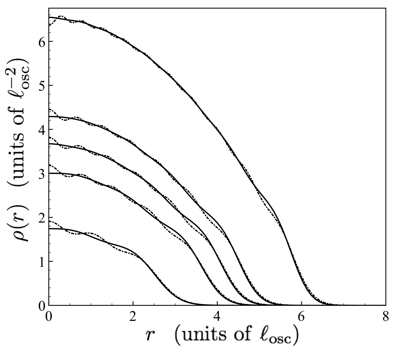
Figure 5: The exact (dot-dashed curves), and TFvW-like self-consistent spatial densities (solid curves), from lowest to highest curves, for $N=30,90,132,182,420$ particles.

More importantly, it is very encouraging to see that the self-consistent spatial densities accurately reproduce the shape of the exact densities as one moves out to the edge of the cloud. For example, the lowest curve in Fig. 5, corresponding to $N=30$ particles, shows excellent agreement with the exact density for $r\gtrsim 2.5$. The fact that the TFvW-like self-consistent densities yield the correct behaviour near the edge of the distribution is a significant result given that it is obtained with no adjustable parameters. To further highlight the quality of the self-consistent TFvW-like theory, we present in Fig. 6 a comparison of the TFvW and TFvW-like spatial densities for $N=30,90,132,182,420$. It is clear that the optimal TFvW densities (dashed curves) exhibit too sharp a decay into the classically forbidden region, as compared to the TFvW-like self-consistent densities (solid curves). In fact, we have examined the TFvW spatial densities for a range of values, $0<\lambda_{\rm vW}\leq 1$, and have found that they cannot provide the correct density profile of the exact densities near the edge of the system. In contrast, the nonlocal TFvW-like theory correctly captures the surface profile of the exact density (see Fig. 5) with no adjustable parameters.

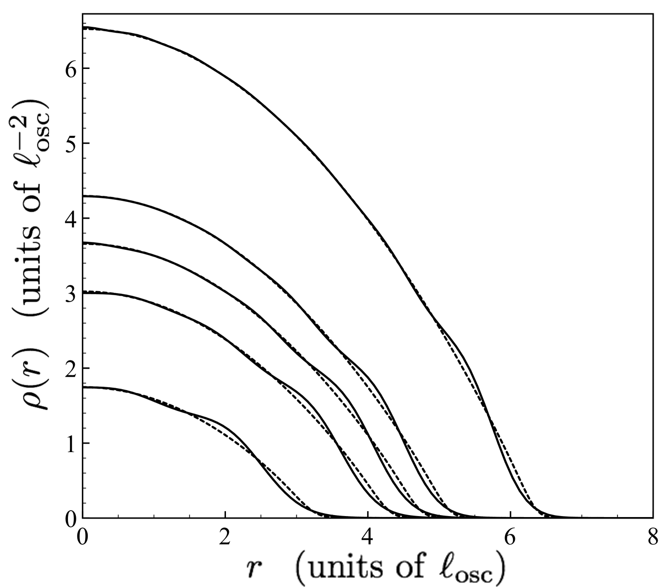
Figure 6: The self-consistent spatial densities from the nonlocal TFvW-like theory (solid curves) and TFvW theory (dashed curves) for $N=30,90,132,182,420$ particles. Note that the TFvW densities are obtained by using an optimal vW coefficient for each particle number ($\lambda_{\rm vW}=0.0568$, 0.0503, 0.0484, 0.0468, 0.0433 for $N=30,90,132,182,420$ particles, respectively).

In order to gain some insight into the differences between the TFvW and TFvW-like spatial densities, we display in Fig. 7 the self-consistent effective potentials, $v_{\rm eff}(r)$, from the two theories. Our first observation is that the oscillatory structure of the TFvW-like $v_{\rm eff}(r)$ manifests itself in the self-consistent TFvW-like spatial density (see, e.g., the lowest set of curves in Fig. 7, where the TFvW-like spatial densities have been overlaid as the dashed-curves). This of course is not surprising, since the effective potential determines the spatial density profile of the system through Equation (68). In addition, both the TFvW and TFvW-like $v_{\rm eff}(r)$ are in good agreement near the centre of the trap, and with increasing particle number, the TFvW-like effective potential closely follows the TFvW curve in the bulk; this agreement explains the similarities between the TFvW and TFvW-like spatial densities displayed in Fig. 6 for large particle numbers. However, as we approach the edge of the system (e.g., for the lowest curves in Fig. 7, $r\gtrsim 2$) the differences in the structure of the effective potentials in the low-density regime are quite dramatic. Specifically, the TFvW-like effective potential develops a local minimum near the edge of the cloud, whereas for the same coordinate range, the TFvW potentials remain comparatively flat. In view of the results presented in Fig. 5, it is clear that the behaviour of the TFvW-like effective potential near the surface of the system is a more accurate representation of the exact effective potential. The other noteworthy feature in the TFvW-like effective potential is the “knee” developing in the very low-density regime, which becomes more prominent as the number of particles is increased. We have numerically determined that this knee-like feature is a result of the nonlocal part of the effective potential, arising specifically from the $\tilde{w}$ term in $\phi(r)$ in Equation (70). While this knee feature is only prominent in the low density regime, its presence appears to be crucial for providing the correct behaviour of the TFvW-like spatial density in the classically forbidden region, $r\gg R_{\rm TF}$. It would be of interest to examine the exact effective potential obtained from the 2D HO KE density functional march , against the TFvW-like effective potentials shown in Figure 7 obtained from the ADA nonlocal KE functional.

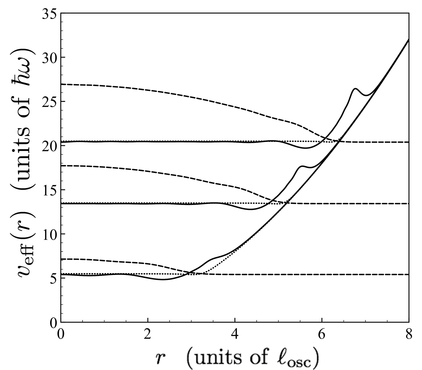
Figure 7: The self-consistent effective potentials for $N=30,182,420$ particles corresponding to the TFvW (dotted curves) and TFvW-like (solid curves). The dashed curves are the self-consistent TFvW-like densities, which have been overlaid to illustrate the way in which $v_{\rm eff}(r)$ determines the density distribution.

IV Closing Remarks

We have applied the ADA in the construction of a nonlocal KE functional, and have used it to formulate a TFvW-like theory for the ground state properties of a 2D inhomogenous Fermi gas. One of our central findings is that the 2D ADA nonlocal KE functional does not admit additional parameters in its definition, in contrast to the situation in 1D and 3D, where there is considerable freedom in specifying the form of the functional. In addition, the ADA naturally leads to a vW term in 2D, which is consistent with what is found in other dimensions. Although such a gradient correction cannot be justified in 2D on the basis of a systematic gradient expansion, it is nevertheless an important component of the nonlocal kinetic energy functional, particularly in the low-density region, where the decay into the classically forbidden region is smooth.

A commonly-used procedure for testing the efficacy of a KE functional is to investigate its ability to generate accurate energies when using the exact density for some model situation. We point out that the results of such a test for a 2D harmonically confined, ideal Fermi gas can be misleading, to wit, in the case of 2D HO confinement, even the crudest, local TF kinetic energy functional, yields superlative results. However, a true measure of the quality of a functional can only be ascertained by examining the nature of the density profiles it produces upon a functional minimization with respect to the density. In this regard, the TF functional demonstratably fails. On the other hand, the fully self-consistent DFT calculations we have performed using the ADA kinetic energy functional yield very good results for the total energy of the harmonically-confined model system. In addition, based on a comparison with exact results, we find that the TFvW-like theory provides a surprisingly good description of the density in the low-density regime.

We have also compared our self-consistent calculations with the results of an earlier 2D TFvW theory in which the vW coefficient is optimized in order to yield the correct total energy. This comparison shows that the local nature of the TFvW KE functional, Eq. (12), is the reason behind the poor description of the surface density profile. Nevertheless, the reasonably good agreement with exact results, along with its simple form, and exceedingly easy numerical implementation, suggest that the 2D TFvW is still a useful tool for the description of inhomogeneous 2D systems, provided one is interested in properties that are relatively insensitive to the local details of the equilibrium spatial density (e.g., total energies, and collective excitations vanzyl1 ; vanzyl2 ; vanzyl3 ; vanzyl4 ).

Finally, we believe that this paper fills a gap in the literature dealing with the DFT of 2D non-uniform Fermi systems. In particular, where standard linear response and semiclassical expansion techniqes in 2D fail to produce gradient corrections associated with spatial inhomogenieties, the ADA naturally allows for the inclusion of beyond LDA physics to the KE functional in a dimensionally independent way. More importantly, the 2D KE functional developed within the ADA has no free parameters, so it may be scrutinized in other systems without the possibility of any “fine tuning”. Our hope is that the nonlocal functional we have presented will stimulate further work toward the development of more accurate KE functionals in low-dimensional Fermi systems. For example, an interesting extension of this work would be to apply the generalization of the ADA developed in Ref. garcia96 to 2D, and examine how the resulting functional improves the determination of the global, and local properties (e.g., shell structure) of the system.

- (1) R. M. Dreizler and E. K.U. Gross, Density Functional Theory: An Approach to the Quantum Many-Body Problem (Springer-Verlag, Berlin, 1990).
- (2) W. Kohn and L. J. Sham, Phys. Rev. 140 A1133 (1965).
- (3) P. Hohenberg and W. Kohn, Phys. Rev. 136, B864 (1964).
- (4) M. Brack and R. K. Bhaduri, Semiclassical Physics, Frontiers in Physics, Vol. 96, Addison-Wesley, Reading, MA (2003).
- (5) E. Wigner, Phys. Rev. 40, 749 (1932).
- (6) J. G. Kirkwood, Phys. Ref. 44, 31 (1933).
- (7) D. A. Kirzhnits, Sov. Phys. JETP 5, 64 (1957).
- (8) B. K. Jennings, Ph.D. thesis, McMaster University (1976, unpublished).
- (9) C. F. von Weizs¬acker, Z. Phys. 96, 431 (1935).
- (10) C. H. Hodges, Can. J. Phys. 51, 1428 (1973).
- (11) P.A.M. Dirac, Proc. Cambridge Philos. Soc. 26, 376 (1930).
- (12) E. Zaremba and H. C. Tso , Phys. Rev. B 49, 8147 (1994).
- (13) E. Zaremba, Phys. Rev. B 53, R10512 (1996).
- (14) A. Chizmeshya and E. Zaremba, Phys. Rev. B 37, 2805 (1988).
- (15) D. J. W. Geldhart, G. Gumbs, Phys. Rev. B 33, 2820 (1986).
- (16) A. Holas, P. M. Koslowski and N. H. March, J. Phys. A: Math. Gen. 24, 4249 (1991).
- (17) L. Salasnich, J. Phys. A: Math. Theor. 40, 9987 (2007).
- (18) M. Koivisto and M. Stott, Phys. Rev. B 76, 195103 (2007).
- (19) B. P. van Zyl, Thomas Fermi von Weizsäcker Hydrodynamics in Low-Dimensional Electronic Systems, Queen’s University Ph. D Thesis (2000).
- (20) B. P. van Zyl, K. Berkane, K. Bencheikh, and A. Farrell, Phys. Rev. B 83, 195136 (2011).
- (21) A. Putaja, E. Räsänen, R. van Leeuwen, J. G. Vilhena, and M. A. L. Marques, Phys. Rev. B 45, 165101 (2012).
- (22) B. P. van Zyl, P. Pisarski, and E. Zaremba, Phys. Rev. A 87, 043614 (2013).
- (23) M. Hochgräfe, B. P. van Zyl, Ch. Heyn, D. Heitmann, and E. Zaremba, Phys. Rev. B. 63, 033316 (2001).
- (24) B. P. van Zyl and E. Zaremba, Phys. Rev. B 63, 245317 (2001).
- (25) B. P. van Zyl, E. Zaremba, and D. A. W. Hutchinson, Phys. Rev. B 61, 2107 (2000).
- (26) B. P. van Zyl and E. Zaremba, Phys. Rev. B 59, 2079 (1999).
- (27) J. A. Alonso and L. A. Girifalco, Phys. Rev. B, 17, 3735 (1978).
- (28) O. Gunnarsson, M. Jonson, and B. I. Lundquist, Phys. Rev. B 20, 3136 (1979).
- (29) C. Herring, Phys. Rev. A 34, 2614 (1986).
- (30) E. Combariz, E. Chacón, and P. Tarazona, Physica A 180, 225 (1992).
- (31) P. García-González, J. E. Alverllos, and E. Chacón, Phys. Rev. A 57, 4192 (1998).
- (32) E. Chacón, J. E. Alvarellos, and P. Tarazona, Phys. Rev. B 32, 7868 (1985).
- (33) P. García-González, J. E. Alvarellos, and E. Chacón, Phys. Rev. A 54 1897 (1996).
- (34) Jeng-Da Chai and J. D. Weeks, Phys. Rev. B 75, 205122 (2007).
- (35) D. García, H. E. Alvarellos, Phys. Rev. A 76, 052504 (2007).
- (36) F. J. Perrot, J. Phys. Condens. Matter 6, 431 (1994).
- (37) Y.A. Wang and M.P. Teter, Phys. Rev. B 45, 13196 (1992).
- (38) Only a truly nonlocal KE functional can satisfy the exact linear response condition, Eq. (16), in two-dimensions.
- (39) S. Stern, Phys. Rev. Lett 18, 546 (1967).
- (40) J. Lindhard, Kgl. Danske Videnskab. Selskab, Mat–Fys. Medd. 28, No. 8 (1954).
- (41) M. Brack and B. P. van Zyl, Phys. Rev. Lett. 86, 1574 (2001)
- (42) P. Shea and B. P. van Zyl, J. Phys. A: Math. Theor. 40, 10589 (2007).
- (43) I. S. Gradshteyn and I. M. Ryzhik, Table of inegrals, series, and products, -th ed. Academic Press Inc., New York (1980).
- (44) These findings are consistent with the numerical work of I. A. Howard and N. H. March, J. Phys. A 43 195301 (2010).
- (45) R. K. Bhaduri and L. F. Zaifman, Can. J. Phys. 57, 1990 (1979); C. Guet and M. Brack, Z. Phys. A 297, 247 (1980).
- (46) B. P. van Zyl, R. K. Bhaduri, A. Suzuki, and M. Brack, Phys. Rev. A 67, 023609 (2003).
- (47) We are limiting our self-consistent calculation to the noninteracting case, so that we can make comparisons with the available exact results. The inclusion of interactions will not alter the general conclusions drawn in this paper. Moreover, eliminating interactions allows us to attribute the oscillatory structure found in the spatial and KE densities directly to the nonlocal KE functional.
- (48) D. Lemoine, J. Chem. Phys. 101, 3936 (1994).
- (49) G. B. Arfken, H. J. Weber, and F. E. Harris, Mathematical Methods for Physicists: A Comprehensive Guide, 7-th ed., Academic Press, Waltham, MA (2012).
- (50) A. Minguzzi, N. H. March, and M. P. Tosi, Eur. Phys. J. D 15, 315 (2001).