Symmetry-protected topological (SPT) states are short-range entangled states with a symmetry $G$. They belong to a new class of quantum states of matter which are classified by the group cohomology ${\cal H}^{d+1}(G,\mathbb{R}/\mathbb{Z})$ in $d$-dimensional space. In this paper, we propose a class of symmetry-protected topological invariants that may allow us to fully characterize SPT states with a symmetry group $G$ (ie allow us to measure the cocycles in ${\cal H}^{d+1}(G,\mathbb{R}/\mathbb{Z})$ that characterize the SPT states). We give an explicit and detailed construction of symmetry-protected topological invariants for 2+1D SPT states. Such a construction can be directly generalized to other dimensions.

Universal symmetry-protected topological invariants
for symmetry-protected topological states

I Introduction

Quantum states of matter have shown a lot of fascinating properties which require a completely new way of understanding. Recent study of long range quantum entanglementChen et al. (2010) (as defined through local unitary (LU) transformations.Levin and Wen (2005); Verstraete et al. (2005); Vidal (2007)) reveal a direct connection between entanglement and gapped phases of quantum matter. The notion of long range entanglement leads to a more general and more systematic picture of gapped quantum phases and their phase transitions.Chen et al. (2010) For gapped quantum systems without any symmetry, their quantum phases can be divided into two classes: short range entangled (SRE) states and long range entangled (LRE) states.

SRE states are states that can be transformed into direct product states via LU transformations. LRE states are states that cannot be transformed into direct product states via LU transformations. There are many types of LRE states that cannot be transformed into each other via the LU transformations. Those different types of LRE states are nothing but the topologically ordered phases. Fractional quantum Hall statesTsui et al. (1982); Laughlin (1983), chiral spin liquids,Kalmeyer and Laughlin (1987); Wen et al. (1989) $Z_{2}$ spin liquids,Read and Sachdev (1991); Wen (1991a); Moessner and Sondhi (2001) non-Abelian fractional quantum Hall states,Moore and Read (1991); Wen (1991b) etc are examples of topologically ordered phases.

For gapped quantum systems with symmetry, the structure of phase diagram is even richer. SRE states now can belong to different phases. The Landau symmetry breaking states belong to this class of phases, where different states are characterized by their different symmetries. However, even if there is no symmetry breaking, the SRE states that have the same symmetry can still belong to different phases.Chen et al. (2011, 2013a, 2012) The 1D Haldane phases for spin-1 chainHaldane (1983); Affleck et al. (1988) and topological insulatorsKane and Mele (2005a); Bernevig and Zhang (2006); Kane and Mele (2005b); Moore and Balents (2007); Fu et al. (2007); Qi et al. (2008) are examples of non-trivial SRE phases that do not break any symmetry. Those phases are beyond Landau symmetry breaking theory since they do not break any symmetry. Those phases are called Symmetry Protected Topological (SPT) phases, which are under intense study recently.Levin and Stern (2009); Lu and Vishwanath (2012); Liu and Wen (2013); Chen and Wen (2012); Hung and Wen (2012); Hung and Wan (2012); Vishwanath and Senthil (2013); Xu (2013); Lu and Lee (2012a); Hung and Wen (2013); Lu and Lee (2012b); Ye and Wen (2013a); Oon et al. (2012); Xu and Senthil (2013); Wang and Senthil (2013); Burnell et al. (2013); Cheng and Gu (2013); Chen et al. (2013b, c); Ye and Wen (2013b); Metlitski et al. (2013); Gu and Levin (2013); Lu and Vishwanath (2013)

We know that topological orderWen (1989); Wen and Niu (1990); Wen (1990) (ie patterns of long-range entanglement) cannot be characterized by the local order parameters associated with the symmetry breaking. We have to use topological probes to characterize/define topological order. It appears that we only need two topological probes to characterize/define 2+1D topological orders: (a) the robust ground state degeneracy that depend on the spatial topologiesWen (1989); Wen and Niu (1990) but cannot be lifted by any small perturbations, (b) the quantized non-Abelian geometric phases from deforming the degenerate ground states.Wen (1990); Keski-Vakkuri and Wen (1993) Using ground state degeneracy and non-Abelian geometric phases to characterize/define topological order is just like using zero-viscosity and quantized vorticity to characterize/define superfluid order. In some sense, the robust ground state degeneracy and the non-Abelian geometric phases (that generate modular representation of the degenerate ground states) can be viewed as a type of “topological order parameters” for topologically ordered states. Those “topological order parameters” are also referred to as topological invariants of topological order.

With the above understanding of topological order, we like to ask: What are the “topological order parameters” or the symmetry-protected topological invariants that can be used to characterize/define SPT states? One way to characterize SPT states is to create a boundary, and then study the boundary properties.Chen et al. (2011); Levin and Gu (2012); Liu and Wen (2013); Chen and Wen (2012); Vishwanath and Senthil (2013); Wang and Senthil (2013); Burnell et al. (2013); Gu and Levin (2013) This approach is very practical since the boundary can be probed in experiments. But it is not convenient theoretically, since the different ways to create the boundary can lead to different boundary properties, even for the same bulk SPT state. Another way to characterize SPT states is to gauge the on-site symmetryLevin and Gu (2012) and use the introduced gauge field as an effective probe for the SPT order.Wen (2013). (See also Ref. Juven, 2013.) This will be the main theme of this paper. In Ref. Wen, 2013, many SPT invariants are discussed and constructed based on the structure of the group cohomology class that described the SPT states. However, the construction in Ref. Wen, 2013 is not systematic and we often fail to find SPT invariants that fully characterize the SPT state. In this paper, we will try to systematically construct SPT invariants that can fully characterize the SPT state.

We find that we can use the introduced gauge field in a SPT state to “simulate” the degenerate ground states of intrinsic topological order. We can even use the introduced gauge field in a SPT state to “simulate” the quantized non-Abelian geometric phases describe by a unitary matrix $U$ from deforming the “simulated” degenerate ground states. We propose an easy way to compute such non-Abelian geometric phases: the matrix elements of $U$ can be computed from the overlap of a “simulated” degenerate ground state and its twist. For example, in 2+1D, we have

$$\langle\alpha|\hat{U}|\beta\rangle=\text{e}^{-L^{2}/\xi^{2}+o(1/L)}U_{\alpha\beta}$$ (1)

where $L^{2}$ is the area of the system, $|\alpha\rangle,|\beta\rangle$ are the “simulated” degenerate ground states, and $\hat{U}$ is the operator that generate the twist (see eqn. (10), eqn. (11), and eqn. (II.3) for more details). The coefficient $1/\xi^{2}$ is not universal, while the factor $U_{\alpha\beta}$, we believe, is universal.Moradi and Wen (2013); He and Wen (2013) We have a similar result for higher dimensions.

We find a direct relation between the quantized non-Abelian geometric phases and the topological partition function on space-time which can be an arbitrary fiber bundle over $S^{1}$. The different choices of the twist $\hat{U}$ correspond to different fiber bundle. This makes us to believeKong and Wen (2013) that the quantized non-Abelian geometric phases from deforming the simulated degenerate ground states are the “topological order parameters” or the SPT invariants that can be used to fully characterize/define SPT states.

II Universal topological invariants of SPT orders

II.1 Symmetry twist

In order to use introduced gauge field to “simulate” the degenerate ground states, let us introduce the notion of “symmetry twist”. We first assume that the 2D lattice Hamiltonian for a SPT state with symmetry $G$ has a form (see Fig. 1)

$$H=\sum_{(ijk)}H_{ijk},$$ (2)

where $\sum_{(ijk)}$ sums over all the triangles in Fig. 1 and $H_{ijk}$ acts on the states on site-$i$, site-$j$, and site-$k$: $|g_{i}g_{j}g_{k}\rangle$. (Note that the states on site-$i$ are labeled by $g_{i}\in G$.) $H$ and $H_{ijk}$ are invariant under the global $G$ transformations.

Then we perform a $G$ transformation, $h\in G$, only in the shaded region in Fig. 1. Such a transformation will change $H$ to $H^{\prime}$. However, only the Hamiltonian terms on the triangles $(ijk)$ across the boundary are changed from $H_{ijk}$ to $H^{\prime}_{h,ijk}$. Since the $g\in G$ transformation is an unitary transformation, $H$ and $H^{\prime}$ have the same energy spectrum. In other words the boundary in Fig. 1 (described by $H^{\prime}_{h,ijk}$’s) do not cost any energy.

Now let us consider a Hamiltonian on a lattice with a “loop” (see Fig. 1)

$$H^{\text{gauged}}_{h}={\sum_{(ijk)}}^{\prime}H_{ijk}+{\sum_{(ijk)}}^{\text{loop}}H^{\prime}_{h,ijk}$$ (3)

where $\sum^{\prime}_{(ijk)}$ sums over the triangles not on the loop and $\sum^{\text{cut}}_{(ijk)}$ sums over the triangles that are divided into disconnected pieces by the loop. We note that the loop carries no energy. The Hamiltonian $H^{\text{gauged}}_{h}$ defines the symmetry twist generated by $h\in G$. We like to point out that the above procedure to obtain $H^{\text{gauged}}_{h}$ is actually the “gauging” of the $G$ symmetry. $H^{\text{gauged}}_{h}$ is a gauged Hamiltonian that contains a locally flat gauge configuration.

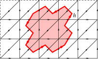
Figure 1: (Color online) A 2D lattice on a torus. A $h\in G$ transformation is performed on the sites in the shaded region. The $h$ transformation changes the Hamiltonian term on the triangles $(ijk)$ across the boundary (the loop) from $H_{ijk}$ to $H^{\prime}_{h,ijk}$.

II.2 Simulating nearly degenerate ground states

Figure 2: (Color online) The Hamiltonian $H^{\text{gauged}}_{h_{x},h_{y}}$ with two symmetry twists $h_{x}$ and $h_{y}$ along the loops in $y$- and $x$- directions respectively. The shaded triangles $(ijk)$ across the the loop contain Hamiltonian terms $H^{\prime}_{h_{x},ijk}$ or $H^{\prime}_{h_{y},ijk}$.

The 2+1D topologically ordered states usually have topologically robust nearly degenerate ground states on torus. Such nearly degenerate ground states can be simulated in SPT states via the symmetry twists discussed above.

To simulate the nearly degenerate ground states on torus, we consider a SPT state on torus with two symmetry twists $h_{x}$ and $h_{y}$ along the loops in $y$- and $x$- directions respectively (see Fig. 2). The resulting Hamiltonian is denoted as $H^{\text{gauged}}_{h_{x},h_{y}}$, and its unique ground state is denoted as $|\Psi_{h_{x},h_{y}}\rangle$.

We note that the loops in $y$- and $x$- directions intersect. In order that the intersecting point does not cost any energy (ie in order for the gauged Hamiltonian to describe a locally flat gauge configuration), we require that

$$[h_{x},h_{y}]=0.$$ (4)

$|\Psi_{h_{x},h_{y}}\rangle$ with commuting $h_{x},h_{y}$ simulates the nearly degenerate group states.

A symmetry twist locally breaks the global symmetry, and group action can be defined on them. In our construction, a twist characterized by a group element $h$ is transformed to $h\to ghg^{-1}$. i.e. The group acts by conjugation. Therefore, twists connected by orbits of the group action falls into the same conjugacy class. This is analogous to the usual quotient group $G/H$ classification of defects, where $H$ is a normal subgroup keeping the defect invariant. It is then clear that the $G$ symmetry implies that the ground states $|\Psi_{h_{x},h_{y}}\rangle$ and $|\Psi_{gh_{x}g^{-1},gh_{y}g^{-1}}\rangle$ of $H^{\text{gauged}}_{h_{x},h_{y}}$ and $H^{\text{gauged}}_{gh_{x}g^{-1},gh_{y}g^{-1}}$ respectively, connected by a group action $I(g),g\in G$, i.e.

$$I(g)|\Psi_{h_{x},h_{y}}\rangle=I_{(gh_{x}g^{-1},gh_{y}g^{-1}),(h_{x},h_{y})}|\Psi_{gh_{x}g^{-1},gh_{y}g^{-1}}\rangle,$$ (5)

for some characteristic $U(1)$ phase $I_{(gh_{x}g^{-1},gh_{y}g^{-1}),(h_{x},h_{y})}$ have exactly the same energy. In an intrinsic topological order constructed from the gauged theory with the same group $G$, it is the equivalence class $\{|\Psi_{gh_{x}g^{-1},gh_{y}g^{-1}}\rangle|g\in G\}$ that corresponds to a single nearly degenerate group state.

If $G$ is Abelian and finite, each equivalent class contains only one state $|\Psi_{h_{x},h_{y}}\rangle$, and the total number of equivalent classes is $|G|^{2}$, where $|G|$ is the number of elements in $G$. This agrees with the topological ground state degeneracy of $G$-gauge theory on torus which is also $|G|^{2}$ if $G$ is Abelian.

II.3 Simulate the non-Abelian geometric phases

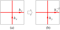
Figure 3: (Color online) (a) A system on a torus with two symmetry twists in $x$- and $y$-directions. Note that the torus has the same size $L$ in $x$- and $y$-directions. (b) The $S$-transformation of the torus, and the resulting new symmetry twists.

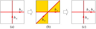
Figure 4: (Color online) (a) A system on a torus with two symmetry twists in $x$- and $y$-directions. Note that the torus has the same size $L$ in $x$- and $y$-directions. (b) The $T$-transformation of the torus, and the resulting new symmetry twists. (c) After local symmetry transformation $h_{x}$ in the shaded region, the symmetry twists in (b) become symmetry twists in $x$- and $y$-directions.

Using the simulated degenerate ground states and assuming that the Hamiltonian is translation invariant, we can also simulate the non-Abelian geometric phases in the topological order. Let $\Psi_{h_{x},h_{y}}(\{g_{i_{x},i_{y}}\})$ be the wave function of $|\Psi_{h_{x},h_{y}}\rangle$:

$$|\Psi_{h_{x},h_{y}}\rangle=\sum_{\{g_{i_{x},i_{y}}\}}\Psi_{h_{x},h_{y}}(\{g_{i_{x},i_{y}}\})|\{g_{i_{x},i_{y}}\}\rangle,$$ (6)

where we have assumed that our system is on a square lattice with periodic boundary condition, and the physical states on each site, $(i_{x},i_{y})$, are labeled by $g_{i_{x},i_{y}}$. The symmetry twists $h_{x},h_{y}$ are given in Fig. 3(a) and 4(a).

Now let us consider the modular transformations of the lattice

$$\begin{pmatrix}i_{x}\\ i_{y}\\ \end{pmatrix}\to W\begin{pmatrix}i_{x}\\ i_{y}\\ \end{pmatrix},\ \ \ \ W\in SL(2,\mathbb{Z}),$$ (7)

which maps the torus to torus. The modular transformations is generated by

$$S_{0}=\begin{pmatrix}0&-1\\ 1&0\\ \end{pmatrix},\ \ \ \ \ T_{0}=\begin{pmatrix}1&1\\ 0&1\\ \end{pmatrix}.$$ (8)

The state $|\Psi_{h_{x},h_{y}}\rangle$ changes under the modular transformation. Let us define

$$|\Psi^{S}_{h_{x},h_{y}}\rangle =\sum_{\{g_{i_{x},i_{y}}\}}\Psi_{h_{x},h_{y}}(\{g_{-i_{y},i_{x}}\})|\{g_{i_{x},i_{y}}\}\rangle,$$

$$|\tilde{\Psi}^{T}_{h_{x},h_{y}}\rangle =\sum_{\{g_{i_{x},i_{y}}\}}\Psi_{h_{x},h_{y}}(\{g_{i_{x}+i_{y},i_{y}}\})|\{g_{i_{x},i_{y}}\}\rangle.$$ (9)

We note that the state $|\Psi^{S}_{h_{x},h_{y}}\rangle$ and the state $|\Psi_{h^{\prime}_{x},h^{\prime}_{y}}\rangle$ have the same symmetry twists if $(h^{\prime}_{x},h^{\prime}_{y})=(h_{y}^{-1},h_{x})$. Thus we define a matrix

$$\hat{S}_{(h^{\prime}_{x},h^{\prime}_{y}),(h_{x},h_{y})}=\delta_{h^{\prime}_{x},h_{y}^{-1}}\delta_{h^{\prime}_{y},h_{x}}\langle\Psi_{h^{\prime}_{x},h^{\prime}_{y}}|\Psi^{S}_{h_{x},h_{y}}\rangle.$$ (10)

However, $|\tilde{\Psi}^{T}_{h_{x},h_{y}}\rangle$ and $|\Psi_{h^{\prime}_{x},h^{\prime}_{y}}\rangle$ always have different symmetry twists (see Fig. 4(b)). To make their symmetry twists comparable, we make an additional local symmetry transformation $h_{x}$ in the shaded region Fig. 4(b), which changes $|\tilde{\Psi}^{T}_{h_{x},h_{y}}\rangle$ to $|\Psi^{T}_{h_{x},h_{y}}\rangle$. Now $|\Psi^{T}_{h_{x},h_{y}}\rangle$ and $|\Psi_{h^{\prime}_{x},h^{\prime}_{y}}\rangle$ have the same symmetry twists if $(h^{\prime}_{x},h^{\prime}_{y})=i(h_{x},h_{y}h_{x})$ (see Fig. 4(c)). Thus we define a matrix

$$\hat{T}_{(h^{\prime}_{x},h^{\prime}_{y}),(h_{x},h_{y})}=\delta_{h^{\prime}_{x},h_{x}h_{y}}\delta_{h^{\prime}_{y},h_{y}}\langle\Psi_{h^{\prime}_{x},h^{\prime}_{y}}|\Psi^{T}_{h_{x},h_{y}}\rangle.$$ (11)

As is evident from the expressions above, for given pair $\{h_{x},h_{y}\}$, it uniquely specifies the values of $\hat{S}$ and $\hat{T}$, since the bra state $\langle\Psi_{h^{\prime}_{x},h^{\prime}_{y}}|$ with non-trivial overlap with the modular transformed state depends solely on the choice of $|\Psi_{h_{x},h_{y}}\rangle$. This suggests that we might as well view $\hat{S}$ and $\hat{T}$ as some functions of $\{h_{x},h_{y}\}$. i.e. $\hat{S}_{(h^{\prime}_{x},h^{\prime}_{y}),(h_{x},h_{y})}=F_{\tilde{S}}(h_{x},h_{y})$ and similarly $\hat{T}_{(h^{\prime}_{x},h^{\prime}_{y}),(h_{x},h_{y})}=F_{\hat{T}}(h_{x},h_{y})$.

Note that both $\hat{S}_{(h^{\prime}_{x},h^{\prime}_{y}),(h_{x},h_{y})}$ and $\hat{T}_{(h^{\prime}_{x},h^{\prime}_{y}),(h_{x},h_{y})}$ depend on the size $L$ of the torus (which is the same in the $x$- and $y$-directions). Here we conjecture that $\hat{S}_{(h^{\prime}_{x},h^{\prime}_{y}),(h_{x},h_{y})}$ and $\hat{T}_{(h^{\prime}_{x},h^{\prime}_{y}),(h_{x},h_{y})}$ have the forms

$$\hat{S}_{(h^{\prime}_{x},h^{\prime}_{y}),(h_{x},h_{y})} =\hskip 1.0pt\mathrm{e}^{-A_{S}L^{2}+o(1/L)}S_{(h^{\prime}_{x},h^{\prime}_{y}),(h_{x},h_{y})},$$

$$\hat{T}_{(h^{\prime}_{x},h^{\prime}_{y}),(h_{x},h_{y})} =\hskip 1.0pt\mathrm{e}^{-A_{T}L^{2}+o(1/L)}T_{(h^{\prime}_{x},h^{\prime}_{y}),(h_{x},h_{y})},$$ (12)

where $A_{S}$ and $A_{T}$ are two complex constants (with positive real parts), and $S_{(h^{\prime}_{x},h^{\prime}_{y}),(h_{x},h_{y})}$ and $T_{(h^{\prime}_{x},h^{\prime}_{y}),(h_{x},h_{y})}$ are topological invariants that are independent of any local perturbations of the Hamiltonian that respect the translation symmetry. This is one of the main results of this paper. It is possible that $S_{(h^{\prime}_{x},h^{\prime}_{y}),(h_{x},h_{y})}$ and $T_{(h^{\prime}_{x},h^{\prime}_{y}),(h_{x},h_{y})}$, together with the group action operator $I(g)$, fully characterize the SPT states with a symmetry group $G$ in 2+1D. In the rest of this paper, we will compute $S$ and $T$ for 2+1D SPT states described by ideal fixed point wave functions.Chen et al. (2011, 2013a, 2012)

III Compute the universal topological invariants for SPT orders

In the previous section, we have introduced the notion of symmetry group action matrix $I(g)$ and modular matrices $S$ and $T$ acting on a basis states containing a pair of twists on a torus in an SPT phase. In this section, we would like to discuss how these quantities are computed in idealized fixed point wave-functions describing an SPT phase, and the procedure to restore the topologically invariant information stored in these objects.

III.1 Twisting the SPT

It is known that the fixed point wavefunction of a SPT is blind to the group cohomology data of the system, whereas that of the related topological gauge theory is a very interesting object. The group cohomology data is revealed in the gauge theory through field configurations consisting of Wilson loops that wind non-trivial cycles. This corresponds to link variables $\prod_{ij\in\textrm{loop}}\mu_{ij}$, where $i,j,\cdots$ are vertices along a loop. If this is a flat connection, and that the loop is contractible, this Wilson loop evaluates to 1. These loops are exactly the gauge theory version of the loops introduced in (3). The only difference is that in a gauge theory these loops are dynamical degrees of freedom that can be excited anywhere, whereas in (3) it appears in designated place.

In the discussion surrounding (3), the manifold is basically assumed open, such that there is a clear notion of a region inside of the given loop and a region outside. More generally, say on a torus or more general higher genus surfaces, by insisting that vertices “inside” a non-contractible loop gets transformed by $h$, we are essentially defining a branch cut along the non-contractible loop, and the field configuration is not single valued. Such configurations are not usually considered in the SPT path-integral, because the path integral over field configuration $g(x)$ includes only single valued maps $g(x)$ to the target space $G$. It is however a well-defined link variable from the point of view of the gauge theory.

To reiterate, these twists correspond to “twisted” boundary condition in the field configuration $g(x)$. In particular, in the case of finite group on a lattice, closed loops are represented by a set of lattice vectors $e=\{e_{x},e_{y}\cdots\}$, which specifies shifts on the lattice that takes one between identified vertices, a Wilson loop in the SPT phase can be implemented by

$$g_{i+e}=g_{i}\times h_{e}.$$ (13)

This is practically how we specify field configuration on the idealized lattice wavefunction corresponding to the transformation effected on the Hamiltonian described in the diagram (2).

The path-integral of the SPT phase now sums over all maps $g(x)$ satisfying the given twisted boundary condition specified above. Schematically, the SPT path-integral would be given by

$$Z_{\textrm{SPT}}=\int\mathcal{D}[g(x)]|_{g_{i+e_{\mu}}=g_{i}\times h_{\mu}}e^{iS[g(x)]}.$$ (14)

This however should be contrasted with the path-integral of the topological gauge theory where all different gauge configurations or Wilson loops have to be summed over. In the SPT path-integral the “Wilson loops” are twisted boundary conditions, and are thus fixed. Such boundary conditions would lead to interesting dependence of the SPT path-integral and ultimately the $S$ and $T$ matrices on the group cohomology data, as we will demonstrate in some simple examples in the following sections.

III.2 Examples for finite groups

In order to set the notations for our results, let us begin with a review of the idealized fixed point wavefunctions on a lattice describing an SPT with global symmetry group $G$.

III.2.1 Some preamble on idealized fixed point wavefunctions

Let us consider the path-integrals, or fixed point wavefunctions in greater detail in the case of finite group $G$ on a discrete lattice. This requires a triangulation of the space-time manifold $M$ which we denote as $M_{\textrm{tri}}$, the space-time complex. The action amplitude is then the product of the amplitude of each $d$- simplex $T_{d}$ of $M_{\textrm{tri}}$. The amplitude $\nu_{d}(\{g_{v_{a}\in T_{d}}\})$ on each $T_{d}$ is a $U(1)$ phase that depends on the “field configuration” $g_{v_{a}}\in G$ and $v_{a}\in T_{d}$ denotes the $d$ vertices on $T_{d}$. As shown in Ref. Chen et al., 2013a and briefly discussed above, these phases $\nu_{d}(\{g_{v_{a}\in T_{d}}\})$ satisfy the $d$-cocycle condition and the distinct equivalence classes in the group cohomology group $\mathcal{H}^{d}(G,U(1))$ corresponds to different phases. To evaluate $\nu_{d}$ on each simplex for a given representative of an equivalence class in $\mathcal{H}^{d}(G,U(1))$, one needs also to assign a local order of the vertices. This gives an orientation to each edge and also determines the orientation of the simplex. Such an order is called a branching structure. The cocycle is therefore a function of the field configurations on the ordered vertices $\nu_{d}(g_{i_{0}},g_{i_{1}},\cdots,g_{i_{d}})$, $i_{0}<i_{1}\cdots<i_{d}$. Such a local ordering can also be obtained if we assign a global ordering to all the vertices in the complex $M_{\textrm{tri}}$. As discussed in the previous section, we would like to evaluate the action amplitude with twisted boundary conditions.

In general, there would be non-trivial cycles in a closed orientable manifold. As we described in the previous section, non-trivial closed loops can be represented by a set of shift vectors $e=\{e_{x},e_{y},\cdots\}$ on the lattice where vertices related by the shift are identified. Let us emphasize that these lattice vectors serve to specify how the multiple (ie infinite in this case) copies of the space-time manifold $M$ is identified and is not related to the lattice discretization in the triangulation $M_{\textrm{tri}}$. In this light, the twisted boundary condition is given by

$$g_{i+e}=g_{i}h_{e},$$ (15)

for a fixed set of group elements $h_{e}$ assigned to each of the $d$ one cycles. The choice for $h_{e}$ along each 1-cycle is not completely arbitrary. Very much like the case of Wilson loops in lattice gauge theory, they have to satisfy consistency conditions. The basic rule is that the aggregate twist element along a contractible loop has to be the identity. For example, on a $d$-torus since $e_{\mu}+e_{\nu}-e_{\mu}-e_{\nu}$ is a contractible loop for any $\mu,\nu\in\{1,\cdots,d\}$, it means $[h_{e_{\mu}},h_{e_{\nu}}]=1$ for all pairs. This is precisely the same condition already described in section 2.

To evaluate the action amplitude therefore, we pick a fundamental region among the multiple copies of space-time manifold introduced. The boundaries of the fundamental region are thus $d-1$ dimensional surfaces with normal vectors given by $e=\{e_{x},e_{y},\cdots\}$. Action amplitudes of simplices lying well within the fundamental region can be evaluated as usual. For a simplex that crosses the boundary with outward normal $\pm e$, the action amplitude is $\nu(\tilde{g}_{i_{1}},\cdots\tilde{g}_{i_{d}})$, such that $\tilde{g}_{i_{n}}=g_{i_{n}}$ for the vertex $i_{n}$ within the fundamental region, but otherwise $\tilde{g}_{i_{n}}=g_{i_{n}}h_{\nu}^{\pm}$ according to the twisted boundary condition Eq. (15).

In other words, in a general $d$-manifold $M$, the twisted boundary condition above where the field is shifted across a closed loop defined by the shift vector $e$ corresponds to introducing some $d-1$ dimensional branch surfaces (whose precise positions are arbitrary and fixed by some chosen convention as in the choice above for a $d$-torus) such that the field acquires a “twist” $h_{e}$ when the cut-surface with normal vector $e$ is crossed.

In order to make direct parallels with the case of lattice gauge theories we also require that the numbering of the vertex $i_{n}$ satisfies a twisted boundary condition

$$i_{n}(v_{a}+e_{i})\to i_{n}+i\times N_{v},$$ (16)

where $N_{v}$ is the total number of vertices in $M_{\textrm{tri}}$. The virtue is that this gives a unique orientation to all the edges if we stay in one fundamental region of the lattice, and that edges that are identified in different unit cells would have consistent orientations. The path-integral of the SPT phase is now given by

$$Z_{\textrm{SPT}}(\{h_{i}\})=|G|^{-N_{v}}\sum_{\{g_{v_{a}}\}}\prod_{k}\{\nu_{d}(\{g_{v_{a}}\}_{T^{k}_{d}})\}^{\epsilon_{k}}$$ (17)

In the presence of these twists $\{h_{i}\}$, the path-integral would depend non-trivially on the cohomology classes.

III.2.2 $d=3$

Having discussed very generally the construction of these twisted path-integrals in general dimensions, let us focus particularly on the interesting case of $d=3$. As a warm up, it is useful to first consider the special case where the three space-time manifold concerned is given by $Y\times S^{1}$, where $Y$ is a 2-sphere with three holes. The triangulation is represented in Fig. 5, where the sphere is represented by the triangle whose three vertices are identified, and the holes by the three edges, and $S^{1}$ corresponds to the vertical edge perpendicular to the triangle.

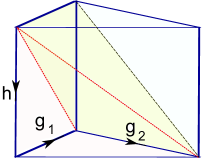
Figure 5: (Color online) The cellurarization into three tetrahedrons of $Y\times S^{1}$.

We can again assign twist boundary conditions on the non-contractible cycles of $Y$.

A group element is assigned to each of the cycles, subjected to the flatness condition on the triangle. The consistency condition also immediately follows:

$$[h,g_{i}]=1.$$ (18)

Again, the above condition is a result of considering the group element assignment to diagonals on any of the vertical rectangles. Since the manifold is open, no summation is required over the group elements, and the path-integral with the orientation assignment as in the figure is given by

$$Z_{Y\times S_{1}}=\frac{\alpha(h,g_{1},g_{2})\alpha(g_{1},g_{2},h)}{\alpha(g_{1},h,g_{2})}\equiv c_{h}(g_{1},g_{2}).$$ (19)

Here for convenience we denote $\nu_{3}(g_{0},g_{1},g_{2},g_{3})\equiv\alpha(g_{0}^{-1}g_{1},g_{1}^{-1}g_{2},g_{2}^{-1}g_{3})$, where the cocycles expressed in the form $\alpha$ is typically used in defining a lattice gauge theory in which gauge degrees of freedom sit on the links connecting the vertices. One important feature to notice is that in the path-integral above the twists on closed loops $h,g_{1},g_{2}$ are not summed over, since they correspond to specific boundary conditions of the field configurations, contrasting what happens in a gauge theory when the link variables are dynamical and has to be summed.

This combination of three cocycles is denoted $c_{h}(g_{1},g_{2})$ because it can be readily shown that it is a 2-cocycle of the group $N_{h}$, where $N_{h}\subset G$ denotes the subgroup whose elements commute with $h$. From the relation between $c_{h}(g_{1},g_{2})$ and the 3-cocycles $\alpha$, we should rewrite $Z_{Y\times S_{1}}=c_{h}^{\epsilon}(g_{1},g_{2})$. If the orientation of the triangle aligns with that of the vertical edge we obtain $\epsilon=+1$, and $\epsilon={\dagger}$ otherwise.

III.2.3 Group action and Modular matrices

As is well known that path-integrals evaluated on an open $d$ space-time manifold with a $d-1$ dimensional boundary surface with specific boundary conditions, we are essentially defining a basis of quantum states in a Hilbert space. Operators acting on this basis of states would appear as a path-integral over a space-time manifold that connects the two different $d-1$ dimensional surfaces where the quantum state is defined. Geometrically, an operator is therefore a cylindrical object with two different boundary conditions at the top and bottom, and whose path-integral is interpreted as the matrix element $M_{\Psi_{1}\Psi_{2}}|\Psi_{1}\rangle\langle\Psi_{2}|$. They are depicted in Fig. 6.

Figure 6: (Color online) An operator acting on a set of basis states defined on a 2d torus. The top and bottom surface rectangles correspond to two states defined on a torus.

Now in particular, we can consider placing the system on a solid torus. The boundary is a two torus which has two non-contractible cycles, although one of which is contractible in the interior of the torus. See Fig. 7.

Figure 7: (Color online) The depiction of a solid torus. The colored surfaces correspond to the position of the branch surfaces across which a vertex field degree of freedom is twisted by a group element. The loop on the surface torus that is contractible in the solid torus extends into a branch surface that ends in the interior of the solid torus. (blue surface)

The path-integral on the solid torus thus defines a basis for the Hilbert space on the surface torus. In particular, the basis is built up by setting different boundary conditions on the torus, including different twisted surface configurations where non-trivial branch cuts are placed on the boundary. These branch cuts extend into branch surfaces inside the solid torus and could end in the interior. Since there are two non-trivial closed cycles, the distinct basis states are specified by the non-trivial twists along each cycle $|\Psi_{h_{x},h_{y}}\rangle$. In the following, for simple notations, we denote each state $|\Psi_{h_{x},h_{y}}\rangle$ simply as

$$|\Psi_{h_{x},h_{y}}\rangle\equiv|h_{x},h_{y}\rangle.$$ (20)

It is a property of the ground state fixed point wavefunction of the SPT phase defined on an open manifold that it is insensitive to the triangulation up to a phase which can be absorbed into the definition of the wavefunction of the state. This fact will be important as we explore quantities that are genuinely free of phase ambiguities. Let us in the meantime make a convenient choice of our basis states with specific branch cuts on the surface torus by picking the simplest possible surface triangulation where there is only one vertex on the boundary, as depicted in Fig. 8. Vertices labeled 1 to 4 are identified. Our choice of basis states is also depicted in Fig. 8.

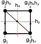
Figure 8: (Color online) Our choice of basis states parametrized by different twists across branch-cuts (dotted lines) on the surface of a solid torus.

ie In the picture we have $|\Psi_{h_{x},h_{y}}(g_{1})\rangle$, where $g_{1}\in G$ is the field degree of freedom sitting at the one vertex of the torus, and $h_{x},h_{y}$ are the twists across the two one-cycle. Note that the path-integral has no dependence on $g_{1}$. Note also that in the topological gauge theory, where the symmetry is gauged, then each ground state on a torus is given by the sum of a state characterized by the pair $|h_{x},h_{y}\rangle$ and all its conjugates $|gh_{x}g^{-1},gh_{y}g^{-1}\rangle$, where $g\in G$. This can be thought of as a projection onto $G$-invariant states. As already emphasized in the previous section, in a SPT the orbits of states under the action of $G$ give rise to a set of physical degenerate states.

The surface torus is invariant under modular transformation. Under such a transformation, it is in fact a reparametrization of the torus, and thus the Hilbert space has to be invariant under the transformation, except that our canonical choice of basis states would be rotated between themselves.

Therefore, we can construct modular transformation matrices that act on the basis states. These transformation matrices can be understood geometrically as a cylindrical object that connect two different solid torus related by a twist. They can thus be expressed as a product of cocycles.

Let us present here the explicit form of both the $S$ and $T$ generators of the modular group, and also the group action operator $I(g)$.

The $S$-transformation corresponds to rotating the torus, where the complex structure $\tau\to\frac{-1}{\tau}$. The $T$-transformation corresponds to a shear transformation where the complex structure $\tau\to\tau+1$. These transformations are depicted in Fig 9 and Fig. 10.

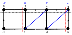
Figure 9: (Color online) The T-transformation involving a reparametrization of the surface torus. The blue labels correspond to the new parametrization, and the blue solid lines outline a parallelogram which is the new choice of unit cell.

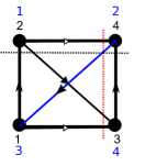
Figure 10: (Color online) The S-transformation involving a reparametrization of the surface torus. The blue labels correspond to the new parametrization, equivalent to rotating the torus by 90 degree. The blue diagonal correspond to the canonical triganulation we have chosen, now with respect to the new parametrization.

The $S$-operator, being a path integral on a cylindrical object that connects the above two parametrizations can thus be triangulated and expressed in terms of the 3-cocycles. The same construction appears also in topological lattice gauge theories, as in Ref. Yidun, . We first define an $S$-operator that involves a non-trivial twist along the vertical direction (along the cylinder) leading to branch cuts in the new surface torus conjugated by element $x\in G$. Choosing $h_{x}=h,h_{y}=g$, we have

$$S(x)|h,g\rangle=\bigg{(}\alpha(hg^{-1},g,x)\alpha(g^{-1}h,gx,x^{-1}g^{-1}x)$$

$$\alpha(gx,x^{-1}g^{-1}x,x^{-1}hx)\alpha(x^{-1}hx,x^{-1}g^{-1}h^{-1}x,x^{-1}hx)$$

$$\alpha(g,x,x^{-1}g^{-1}hx)\bigg{)}$$

$$\bigg{(}\alpha(g,g^{-1}h,x)\alpha(x,x^{-1}hx,x^{-1}g^{-1}x)\bigg{)}^{-1}$$

$$|x^{-1}g^{-1}x,x^{-1}hx\rangle$$ (21)

Similarly, we can read off the T-matrix with vertical twist $x$ as

$$T(x)|h,g\rangle=\bigg{(}\alpha(hg^{-1},g,x)\alpha(hg^{-1},gx,x^{-1}g^{-1}x)$$

$$\alpha(g,x,x^{-1}hg^{-1}x)\alpha(gx,x^{-1}g^{-1}x,x^{-1}hx)\bigg{)}$$

$$\bigg{(}\alpha(g,hg^{-1},x)\alpha(x,x^{-1}hx,x^{-1}g^{-1}x)$$

$$\alpha(x^{-1}g^{-1}x,x^{-1}ghx,x^{-1}g^{-1}x)\bigg{)}^{-1}$$

$$|x^{-1}hx,x^{-1}ghx\rangle$$ (22)

The group action matrix $I(x)$ on the other hand preserves the parametrization of the surface tori, but introduces a vertical $x$ twist, leading to a conjugation of the branch cuts on the surface tori. Explicitly, it is given by

$$I(x)|h,g\rangle=\bigg{(}\alpha(g^{-1}h,g,x)\alpha(g^{-1}h,x,x^{-1}gx)^{-1}$$

$$\alpha(x,x^{-1}g^{-1}hx,x^{-1}gx)\alpha(x,x^{-1}gx,x^{-1}g^{-1}hx)^{-1}$$

$$\alpha(g,x,x^{-1}g^{-1}hx)\alpha(g,g^{-1}h,x)^{-1}\bigg{)}$$

$$|x^{-1}hx,x^{-1}gx\rangle$$ (23)

Since the $S(x)$ and $T(x)$ transformation corresponds to a reparametrization of the torus (in conjunction with shifting the jumps across the branch surfaces by conjugating by $x$), the position of the branch cuts essentially did not move. They only appear different because we have made a different choice of the unit cell after the reparametrization. Another way to view the transformation is that it maps the three one cycles $[v_{1}v_{2}]$, $[v_{2}v_{3}]$ and $[v_{3}v_{4}]$ to another three, $v_{1}^{\prime}v_{2}^{\prime}$, $v_{2}^{\prime}v_{3}^{\prime}$ and $v_{3}^{\prime}v_{4}^{\prime}$ according to the new parametrization as demonstrated in Fig. (10) and Fig. (9). We could easily rearrange the branch cuts so that they take the same canonical shape with respect to the new unit cell, but the twist is shifted by suitable group elements.

Note that $S(x)=S(1)I(x)$ and similarly $T(x)=T(1)I(x)$.

III.3 Caution: Fixing phase ambiguity and true topological invariants

We would like to pause here and deal with a very important issue: as already noted above, there are phase ambiguities in our choice of basis states. Therefore the $I,S$ and $T$ matrix components are generally ill defined quantities! There are two sources of phase ambiguities. First, the three cocycles $\alpha$ are subjected to an ambiguity. They can be rescaled by a coboundary built on 2-cochains $\beta(g,h)$ as follows

$$\alpha^{\prime}(g,h,k)=\frac{\beta(g,hk)\beta(h,k)}{\beta(g,h)\beta(gh,k)}\alpha(g,h,k).$$ (24)

Upon rescaling, $S(x)$ and $T(x)$ are rescaled as follows

$$\langle g^{-1},h^{-1}|S(x)|h,g\rangle\to\langle h,g^{-1}|S(x)|g,h\rangle$$

$$\frac{\beta(g,g^{-1}h)}{\beta(g^{-1}h,g)}\frac{\beta(x^{-1}h^{-1}g^{-1}x,x^{-1}hx)}{\beta(x^{-1}hx,x^{-1}h^{-1}g^{-1}x)}$$ (25)

and

$$\langle x^{-1}hx,x^{-1}ghx|T(x)|h,g\rangle\to\langle x^{-1}hx,x^{-1}ghx|T(x)|g,h\rangle$$

$$\frac{\beta(g,g^{-1}h)}{\beta(g^{-1}h,g)}\frac{\beta(x^{-1}g^{-1}x,x^{-1}ghx)}{\beta(x^{-1}ghx,x^{-1}g^{-1}x)}.$$ (26)

Similarly,

$$\langle x^{-1}gx,x^{-1}hx|I(x)|g,h\rangle\to\langle x^{-1}gx,x^{-1}hx|I(x)|g,h\rangle$$

$$\frac{\beta(g,g^{-1}h)\beta(x^{-1}g^{-1}hx,x^{-1}gx)}{\beta(g^{-1}h,g)\beta(x^{-1}gx,x^{-1}g^{-1}hx)}.$$ (27)

This suggests that the surface states is simply rescaled by

$$|h,g\rangle\to\frac{\beta(g,hg^{-1})}{\beta(g^{-1}h,g)}|h,g\rangle.$$ (28)

Second, as noted already earlier, we have picked a particular triangulation of our tori. For a different choice of triangulation, that corresponds to filling in extra 3-cocycles $\alpha$. To illustrate that, consider a small change in triangulation in which we replace the solid line joining vertices 2 and 3 by one which joins vertices 1 and 4 in figure 8. This change of triangulation would amount to an extra factor given by $\alpha(h_{y},h_{y}^{-1}h_{x},h_{y})$, which originates from fitting an extra three tetrahedral on the surface of the torus.

The matrix elements of $I(x),S(x)$ and $T(x)$ therefore generally suffers from these phase ambiguities, since they correspond to overlaps of wavefunctions each plagued by phase ambiguities.

A natural way to construct invariant quantities is to consider combinations of $I(x),S(x),T(x)$ that generate a closed orbit in the basis states. As shown in figure 11, a closed orbit connects the same state so that any phase ambiguity would be canceled out between the state and its own complex conjugate. One salient example is the combination $(ST)^{3}$. What does this combination of wavefunction overlaps correspond to from the perspective of path-integrals of topological theories? This in fact is precisely the path-integral over a closed manifold. It is well known that a three-manifold $M$ can be decomposed into two “handle-bodies”, $M_{1},M_{2}$ of genus $g$ by cutting $M$ along a genus $g$ surface. This is known as ’Heegard splitting’. To reproduce $M$, the surfaces of $M_{1},M_{2}$ have to be identified in a non-trivial way. In particular, for $g=1$, the non-trivial identification correspond precisely to doing modular transformations, $S,T$ on the surface torus of $M_{1}$ before gluing with $M_{2}$. Therefore, path-integrals on such an $M$ in topological quantum field theories take precisely the form

$$Z_{M}=\sum_{|\Psi\rangle}\langle\Psi|\Gamma|\Psi\rangle,\qquad\Gamma\in SL(2,\mathbb{Z}),$$ (29)

where $|\Psi\rangle$ is the quantum state defined by the path-integral on the open manifolds $M_{1},M_{2}$ , and $Z_{M}$ is the overlap of the same quantum state after insertion of modular transformation operators $\Gamma$, which are combinations of $S$ and $T$. This is indeed what the wavefunctions overlap computes, in which the $M_{1}$, and $M_{2}$ each corresponds to a $T^{2}\times\mathbb{R}$. In the case of topological gauge theories, we project $|\Psi\rangle$ to a gauge invariant state, by the projector $\sum_{x\in G}I(x)$, and then finally, we also sum over all the states $|\Psi\rangle$. In the case of SPT phase however, no such projection is necessary, and the basis states with given twists $h,g$ are background configurations that should not be summed over. We can thus keep $I(x)$ as an extra operator in our toolbox in addition to $S$ and $T$, which we could use to operate on our basis states defined on the surface torus on $M_{1}$, before taking overlap with the state defined on the surface of $M_{2}$. Therefore, our wavefunction overlaps are precisely path-integrals of the topological theory underlying the SPT phase over some closed manifold $M$.

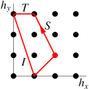
Figure 11: (Color online) $h_{x},h_{y}$ describe the symmetry twists in $x$ and $y$ directions, which label the simulated degenerate ground states on a torus. The action of the $S$ , $T$ and $I$ change one simulated degenerate ground state to another. A closed orbit can be generated by repeated actions of the $S$ , $T$ and $I$ operators.

III.3.1 $\mathbb{Z}_{N}$

Consider specifically $\mathbb{Z}_{N}$ groups. The 3-cocycles of $\mathbb{Z}_{N}$ is given by Moore and Seiberg (1989)

$$\alpha_{k}(g_{1},g_{2},g_{3})=\exp(\frac{2\pi ik\bar{g}_{1}}{N^{2}}(\bar{g}_{2}+\bar{g}_{3}-\overline{(g_{2}+g_{3})})),$$ (30)

for some appropriate $k\in\mathbb{Z}$, and $g_{i}\in\mathbb{Z}_{N}$, and $\bar{x}=x\,\,\,\textrm{mod}\,\,N$ for $x\in\mathbb{Z}$. There are altogether $N$ distinct choices of $k$ that give rise to representatives of the $N$ different group cohomology classes in $H^{3}(\mathbb{Z}_{N},U(1))$. However, this gives $I(x)=1$ identically, independently of the choices of branch cuts $h,g$, or the choice of 3-cocycle specified by $k$.

Let us also inspect the form of the $S$ and $T$ matrix of $\mathbb{Z}_{N}$. For concreteness, let us look at a few simple cases. Substituting into the cocycles, we have, say for $N=2$ the following non-vanishing components:

$$\left(\begin{tabular}[]{cc}$\langle 0,0|\,S(1)\,|0,0\rangle$&$\langle 1,0|\,S(1)\,|0,1\rangle$\\ $\langle 0,1|\,S(1)\,|1,0\rangle$&$\langle 1,1|\,S(1)\,|1,1\rangle$\end{tabular}\right)=$$ (33)

$$\left(\begin{tabular}[]{cc}1&$(-1)^{k}$\\ $(-1)^{k}$&$(-1)^{k}$\end{tabular}\right).$$ (36)

Similarly

$$\left(\begin{tabular}[]{cc}$\langle 0,0|\,T(1)\,|0,0\rangle$&$\langle 0,1|\,T(1)\,|0,1\rangle$\\ $\langle 1,1|\,T(1)\,|1,0\rangle$&$\langle 1,0|\,T(1)\,|1,1\rangle$\end{tabular}\right)=$$ (39)

$$\left(\begin{tabular}[]{cc}1&$1$\\ $1$&$(-1)^{k}$\end{tabular}\right)$$ (42)

Just to give an example where $g^{-1}\neq g$, we inspect also the form of $N=3$, which evaluates to

$$\left(\begin{tabular}[]{ccc}$\langle 0,0|\,S(1)\,|0,0\rangle$&$\langle 2,0|\,S(1)\,|0,1\rangle$&$\langle 1,0|\,S(1)\,|0,2\rangle$\\ $\langle 0,1|\,S(1)\,|1,0\rangle$&$\langle 2,1|\,S(1)\,|1,1\rangle$&$\langle 1,1|\,S(1)\,|1,2\rangle$\\ $\langle 0,2|\,S(1)\,|2,0\rangle$&$\langle 2,2|\,S(1)\,|2,1\rangle$&$\langle 1,2|\,S(1)\,|2,2\rangle$\end{tabular}\right)=$$ (46)

$$\left(\begin{tabular}[]{ccc}1&$\exp(\frac{2ik\pi}{3})$&$\exp(\frac{4ik\pi}{3})$\\ $\exp(\frac{4ik\pi}{3})$&$\exp(\frac{2ik\pi}{3})$&$\exp(\frac{4ik\pi}{3})$\\ $\exp(\frac{2ik\pi}{3})$&$\exp(\frac{4ik\pi}{3})$&$\exp(\frac{2ik\pi}{3})$\end{tabular}\right).$$ (50)

Correspondingly,

$$\left(\begin{tabular}[]{ccc}$\langle 0,0|\,T(1)\,|0,0\rangle$&$\langle 0,1|\,T(1)\,|0,1\rangle$&$\langle 0,2|\,T(1)\,|0,2\rangle$\\ $\langle 1,1|\,T(1)\,|1,0\rangle$&$\langle 1,2|\,T(1)\,|1,1\rangle$&$\langle 1,0|\,T(1)\,|1,2\rangle$\\ $\langle 2,2|\,T(1)\,|2,0\rangle$&$\langle 2,0|\,T(1)\,|2,1\rangle$&$\langle 2,1|\,T(1)\,|2,2\rangle$\end{tabular}\right)=$$ (54)

$$\left(\begin{tabular}[]{ccc}1&$1$&$1$\\ $\exp(\frac{2ik\pi}{3})$&$1$&$1$\\ $\exp(\frac{4ik\pi}{3})$&$\exp(\frac{4ik\pi}{3})$&$1$\end{tabular}\right).$$ (58)

These quantities, as we discussed, are subjected to rescaling. There is however a very convenient set of invariants for cyclic groups. Consider acting the operator $T$ on a state $N$ times, where $N$ is the order of the group– that necessarily takes us back to the same state. In the case of $\mathbb{Z}_{N}$, this gives

$$\langle h,g|T^{N}|h,g\rangle=\exp(\frac{2\pi i(h-1)^{2}k}{N}),$$ (59)

where $k$ is the parameter specifying the 3-cocycle as we described above. This quantity turns out to be sufficient to distinguish all the different $\mathbb{Z}_{N}$ SPT phases! Similar observations can be found in Ref. Zaletel, . The combination $(ST)^{3}$ however evaluates to 1 always.

III.3.2 $\mathbb{Z}_{N}\times\mathbb{Z}_{N}\times\mathbb{Z}_{N}$

The group elements of the group is denoted by a “three-vector” $g=(g_{1},g_{2},g_{3})$. The cohomology group $\mathcal{H}^{3}(\mathbb{Z}_{N}^{3},U(1))$ has seven generators. Six of them involves only two of the three $\mathbb{Z}_{N}$, which lead to trivial results. The interesting generator intertwines the three $\mathbb{Z}_{N}$. The corresponding topological gauge theory contains non-Abelian anyons. This set of cocycles takes the following form:

$$\alpha_{k}(h,g,l)=\exp(\frac{2\pi ki}{N}h_{1}g_{2}l_{3}).$$ (60)

Note that the action of $I(x)$ becomes $x$ dependent for this set of cocycles.

Evaluating on $T^{2}\times S^{1}$ gives

$$Z_{T^{2}\times S^{1}}(h,g,x)_{\alpha_{k}}=\exp(\frac{2\pi ki}{N}(h.g\times x))$$

$$=\langle h,g|\,I(x)\,|h,g\rangle,$$ (61)

where $[x,g]=[x,h]=[h,g]=1$, and $h.g\times x=\epsilon_{abc}h_{a}g_{b}x_{c}$. In this case therefore, we find that each element of $I(x)$ is a topological invariant capable of distinguishing all these non-trivial 3-cocycles.

We can also evaluate $S(1)$ and $T(1)$. In fact, for $N=2$, $T(1)$ simplifies to

$$\langle h,gh|T(1)|h,g\rangle=\exp\left(\pi ki(h_{1}g_{2}g_{3}+h_{2}g_{1}g_{3}+h_{3}g_{1}g_{2})\right).$$ (62)

Similarly, $S(1)$ is given by

$$\langle g^{-1},h|S(1)|h,g\rangle=\exp\bigg{(}\pi ki(g_{1}g_{2}g_{3}+$$

$$h_{1}h_{2}h_{3}+h_{1}g_{2}g_{3}+g_{1}g_{2}h_{3}+h_{1}g_{2}h_{3})\bigg{)}.$$ (63)

In this case of course the matrix elements of $T^{N}$ are again topological invariants. With $I(x)$ and the matrix elements of $T^{N}$ one can distinguish all possible SPT phases with $\mathbb{Z}_{N}\times\mathbb{Z}_{N}\times\mathbb{Z}_{N}$ symmetries.

III.3.3 Some examples of non-Abelian groups

Let us also inspect some simple cases with non-Abelian symmetry groups. In particular, the simplest such example is the Dihedral group $D_{N}$, for $N$ odd. The $2N$ group elements can be represented as a pair $(A,a)$, where $A\in\{0,1\}$, and $a\in\{0,\cdots,N-1\}$. Group product is given by

$$(A,a)\times(B,b)=((A+B)_{\textrm{Mod}\,2},((-1)^{B}a+b)_{\textrm{Mod}\,N}.$$ (64)

The group cocycles are given by

$$\alpha_{k}(g,h,l)=$$

$$\exp\bigg{(}\frac{2\pi ik}{N^{2}}\big{(}(-1)^{H+L}g[(-1)^{L}h+l-((-1)^{L}h+l)_{\textrm{Mod}\,N}]$$

$$+\frac{N^{2}GHL}{2}\big{)}\bigg{)},$$ (65)

where as explained above a group element $g$ corresponds to the pair $(G,g)$, and with an abuse of notation we use the same symbol $g$ also for the second component in the pair, where it is $\in\mathbb{Z}_{N}$.

Evaluated on $T^{2}\times S^{1}$, one again requires that the monodromies across each of the branch-cuts, given by $h,g,x$ have to be mutually commuting. In the Dihedral groups where $N$ is odd, two elements $g_{1}$ given by $(G_{1},g_{1})$, and $g_{2}$, corresponding to $(G_{2},g_{2})$ are mutually commuting if and only if they belong to one of the following situations: (1) they are both in the $Z_{N}$ subgroup where $G_{1}=G_{2}=0$; (2) if $g_{1}$ and $g_{2}$ are the same group element; (3) either $g_{1}$ or $g_{2}$ is the identity element $(0,0)$. As a result

$$\frac{\alpha_{k}(g,h,l)}{\alpha_{k}(g,l,h)}=1$$ (66)

for any $k$ if $g,h,l$ are mutually commuting. As a result, it is also clear from Eqn. (III.2.3) that the partition function on $T^{2}\times S^{1}$ is unity for any set of allowed branch cuts.

We could also look at some examples of $I(x)$. It is not hard to check that for odd values of $N$

$$\langle x^{-1}hx,x^{-1}gx|I(x)|h,g\rangle=\exp\bigg{(}\frac{2\pi ki(-1)^{G+X}}{N^{2}}\big{[}$$

$$(g^{-1}h)<(-1)^{X}g+x(1-(-1)^{G})>-$$

$$(-1)^{H}g<(-1)^{X}g^{-1}h+x(1-(-1)^{G+H})>\big{]}\bigg{)},$$ (67)

where the pointed bracket above means $<n>=n-(n)_{\textrm{Mod}\,N}$. The $T(1)$ matrix can be simplified to

$$\langle h,gh|T(1)|h,g\rangle=\alpha(g,g^{-1},h)\alpha(g^{-1},h,g)\alpha(h,g,g^{-1})$$ (68)

and the corresponding $S(1)$ can be massaged to the form

$$\langle g^{-1},h|S(1)|h,g\rangle=\alpha(h,g^{-1},h)\alpha(g^{-1}h,g,g^{-1}h)\alpha(h,g^{-1}h^{-1},h).$$ (69)

In this case, the operator $S(1)$ acting on basis states with $h=g=\{1,a\}$ already forms closed orbits. Therefore each matrix element, which evaluates to the following

$$\langle h,g|\hat{S}(1)|h,g\rangle|_{h=g=(1,a)}=(-1)^{k},$$ (70)

is a topological invariant.

This only distinguishes $k$ even from $k$-odd 3-cocycles. Similar to cyclic groups, one can also inspect $T^{N}$, acting on states $|h,g\rangle$ such that $h,g$ lives in the $\mathbb{Z}_{N}$ subgroup, taking the form $\{0,a\}$. In this case, $T^{N}$ evaluates precisely to the same value as in (59), with $h$ replaced by $a$ for the element $h=\{0,a\}$. Here $(ST)^{3}$ again evaluates to 1 identically.

IV Summary

In this paper, we propose a systematic way to construct ‘order parameters’ of SPT phases, by exploiting the relationship between an SPT phase and the corresponding intrinsic topological order obtained by gauging the global symmetry described in Ref. Levin and Gu, 2012 .

To simulate the effect of gauging, the idea of the symmetry twist is introduced. Symmetry twists are generated by symmetry transformations performed in a restricted region. The boundary of such a region would play the analogous role of a Wilson line in a topological gauge theory, although in contrast to Wilson lines in a gauge theory, these twists are not dynamical excitations, but background defects.

In the special case of a 2+1 d SPT we can consider putting the system on a torus, ie one that satisfies periodic boundary conditions. States with symmetry twists wrapping the two cycles on the torus can be constructed, leading to a set of almost degenerate basis states. This is again analogous to the situation of a gauge theory with non-trivial Wilson lines. Modular transformation on a torus, corresponding to a reparametrization of the lattice on the torus, can be performed, which would take us to a different basis state, so does a global symmetry transformation. One could consider overlaps of the wavefunctions between a state $|\alpha\rangle$ with some given symmetry twists and a modular and global symmetry transformed version of another state $|\beta\rangle$:

$$\langle\alpha|\hat{U}|\beta\rangle=\text{e}^{-L^{2}/\xi^{2}+o(1/L)}U_{\alpha\beta}.$$ (71)

We conjecture that the factor $U_{\alpha\beta}$ is universal which can be used to characterize the SPT states.

These wavefunction overlaps can be understood as path-integrals of the SPT phase on a three manifold with two boundaries, where each boundary is our torus, which is a constant time slice on which we define our states. These wavefunction overlaps therefore generally suffer from a phase ambiguity, since they are not invariant upon rescaling each basis state with an arbitrary phase. To construct truly universal topological invariants, we further consider closed orbits of the modular transformations. ie We systematically look for combinations of these modular transformations and global symmetry transformations on our basis states such that it keeps the states invariant up to an overall phase.

These overall phases generated by closed orbits of transformations are the topological invariants that we set out to find: like Berry phases, they are independent of any rescaling of our basis states by arbitrary phases. We demonstrate how in various simple symmetry groups, both Abelian and non-Abelian, such closed orbits can be constructed and how they can be extracted using idealized fixed point wavefunctions. It is amusing that, as explained in the text, these special wavefunction overlaps are equivalent to path-integral in some highly non-trivial closed manifold. In the examples we explored in detail, the precise combination of modular transformations leading to closed orbits are generically dependent on the symmetry group involved, and in all the discrete symmetry groups we have considered, there are enough closed orbits that distinguish all the distinct SPT phases with the given symmetry classified in Ref. Chen et al., 2012. This supports the conjecture that our constructed topological invariants fully characterize the SPT states.

LYH would like to acknowledge useful discussions with Yidun Wan. This research is supported by NSF Grant No. DMR-1005541, NSFC 11074140, and NSFC 11274192. It is also supported by the John Templeton Foundation. Research at Perimeter Institute is supported by the Government of Canada through Industry Canada and by the Province of Ontario through the Ministry of Research. The research of LYH is supported by the Croucher Foundation.

References

- Chen et al. (2010) X. Chen, Z.-C. Gu, and X.-G. Wen, Phys. Rev. B 82, 155138 (2010), eprint arXiv:1004.3835.
- Levin and Wen (2005) M. Levin and X.-G. Wen, Phys. Rev. B 71, 045110 (2005), eprint cond-mat/0404617.
- Verstraete et al. (2005) F. Verstraete, J. I. Cirac, J. I. Latorre, E. Rico, and M. M. Wolf, Phys. Rev. Lett. 94, 140601 (2005).
- Vidal (2007) G. Vidal, Phys. Rev. Lett. 99, 220405 (2007).
- Tsui et al. (1982) D. C. Tsui, H. L. Stormer, and A. C. Gossard, Phys. Rev. Lett. 48, 1559 (1982).
- Laughlin (1983) R. B. Laughlin, Phys. Rev. Lett. 50, 1395 (1983).
- Kalmeyer and Laughlin (1987) V. Kalmeyer and R. B. Laughlin, Phys. Rev. Lett. 59, 2095 (1987).
- Wen et al. (1989) X.-G. Wen, F. Wilczek, and A. Zee, Phys. Rev. B 39, 11413 (1989).
- Read and Sachdev (1991) N. Read and S. Sachdev, Phys. Rev. Lett. 66, 1773 (1991).
- Wen (1991a) X.-G. Wen, Phys. Rev. B 44, 2664 (1991a).
- Moessner and Sondhi (2001) R. Moessner and S. L. Sondhi, Phys. Rev. Lett. 86, 1881 (2001).
- Moore and Read (1991) G. Moore and N. Read, Nucl. Phys. B 360, 362 (1991).
- Wen (1991b) X.-G. Wen, Phys. Rev. Lett. 66, 802 (1991b).
- Chen et al. (2011) X. Chen, Z.-X. Liu, and X.-G. Wen, Phys. Rev. B 84, 235141 (2011), eprint arXiv:1106.4752.
- Chen et al. (2013a) X. Chen, Z.-C. Gu, Z.-X. Liu, and X.-G. Wen, Phys. Rev. B 87, 155114 (2013a), eprint arXiv:1106.4772.
- Chen et al. (2012) X. Chen, Z.-C. Gu, Z.-X. Liu, and X.-G. Wen, Science 338, 1604 (2012), eprint arXiv:1301.0861.
- Haldane (1983) F. D. M. Haldane, Physics Letters A 93, 464 (1983).
- Affleck et al. (1988) I. Affleck, T. Kennedy, E. H. Lieb, and H. Tasaki, Commun. Math. Phys. 115, 477 (1988).
- Kane and Mele (2005a) C. L. Kane and E. J. Mele, Phys. Rev. Lett. 95, 226801 (2005a), eprint cond-mat/0411737.
- Bernevig and Zhang (2006) B. A. Bernevig and S.-C. Zhang, Phys. Rev. Lett. 96, 106802 (2006).
- Kane and Mele (2005b) C. L. Kane and E. J. Mele, Phys. Rev. Lett. 95, 146802 (2005b), eprint cond-mat/0506581.
- Moore and Balents (2007) J. E. Moore and L. Balents, Phys. Rev. B 75, 121306 (2007), eprint cond-mat/0607314.
- Fu et al. (2007) L. Fu, C. L. Kane, and E. J. Mele, Phys. Rev. Lett. 98, 106803 (2007), eprint cond-mat/0607699.
- Qi et al. (2008) X.-L. Qi, T. Hughes, and S.-C. Zhang, Phys. Rev. B 78, 195424 (2008), eprint arXiv:0802.3537.
- Levin and Stern (2009) M. Levin and A. Stern, Phys. Rev. Lett. 103, 196803 (2009), eprint arXiv:0906.2769.
- Lu and Vishwanath (2012) Y.-M. Lu and A. Vishwanath, Phys. Rev. B 86, 125119 (2012), eprint arXiv:1205.3156.
- Liu and Wen (2013) Z.-X. Liu and X.-G. Wen, Phys. Rev. Lett. 110, 067205 (2013), eprint arXiv:1205.7024.
- Chen and Wen (2012) X. Chen and X.-G. Wen, Phys. Rev. B 86, 235135 (2012), eprint arXiv:1206.3117.
- Hung and Wen (2012) L.-Y. Hung and X.-G. Wen (2012), eprint arXiv:1211.2767.
- Hung and Wan (2012) L.-Y. Hung and Y. Wan, Phys. Rev. B 86, 235132 (2012), eprint arXiv:1207.6169.
- Vishwanath and Senthil (2013) A. Vishwanath and T. Senthil, Phys. Rev. X 3, 011016 (2013), eprint arXiv:1209.3058.
- Xu (2013) C. Xu, Phys. Rev. B 87, 144421 (2013), eprint arXiv:1209.4399.
- Lu and Lee (2012a) Y.-M. Lu and D.-H. Lee (2012a), eprint arXiv:1210.0909.
- Hung and Wen (2013) L.-Y. Hung and X.-G. Wen, Phys. Rev. B 87, 165107 (2013), eprint arXiv:1212.1827.
- Lu and Lee (2012b) Y.-M. Lu and D.-H. Lee (2012b), eprint arXiv:1212.0863.
- Ye and Wen (2013a) P. Ye and X.-G. Wen, Phys. Rev. B 87, 195128 (2013a), eprint arXiv:1212.2121.
- Oon et al. (2012) J. Oon, G. Y. Cho, and C. Xu (2012), eprint arXiv:1212.1726.
- Xu and Senthil (2013) C. Xu and T. Senthil (2013), eprint arXiv:1301.6172.
- Wang and Senthil (2013) C. Wang and T. Senthil (2013), eprint arXiv:1302.6234.
- Burnell et al. (2013) F. J. Burnell, X. Chen, L. Fidkowski, and A. Vishwanath (2013), eprint arXiv:1302.7072.
- Cheng and Gu (2013) M. Cheng and Z.-C. Gu (2013), eprint arXiv:1302.4803.
- Chen et al. (2013b) X. Chen, F. Wang, Y.-M. Lu, and D.-H. Lee (2013b), eprint arXiv:1302.3121.
- Chen et al. (2013c) X. Chen, Y.-M. Lu, and A. Vishwanath (2013c), eprint arXiv:1303.4301.
- Ye and Wen (2013b) P. Ye and X.-G. Wen (2013b), eprint arXiv:1303.3572.
- Metlitski et al. (2013) M. A. Metlitski, C. L. Kane, and M. P. A. Fisher (2013), eprint arXiv:1302.6535.
- Gu and Levin (2013) Z.-C. Gu and M. Levin (2013), eprint arXiv:1304.4569.
- Lu and Vishwanath (2013) Y.-M. Lu and A. Vishwanath (2013), eprint arXiv:1302.2634.
- Wen (1989) X.-G. Wen, Phys. Rev. B 40, 7387 (1989).
- Wen and Niu (1990) X.-G. Wen and Q. Niu, Phys. Rev. B 41, 9377 (1990).
- Wen (1990) X.-G. Wen, Int. J. Mod. Phys. B 4, 239 (1990).
- Keski-Vakkuri and Wen (1993) E. Keski-Vakkuri and X.-G. Wen, Int. J. Mod. Phys. B 7, 4227 (1993).
- Levin and Gu (2012) M. Levin and Z.-C. Gu, Phys. Rev. B 86, 115109 (2012), eprint arXiv:1202.3120.
- Wen (2013) X.-G. Wen (2013), eprint arXiv:1301.7675.
- Juven (2013) L. -H. Santos and J. Wang Phys. Rev. B 89 195122 (2014).
- Moradi and Wen (2013) H. Moradi and X.-G. Wen, arXiv:1401.0518 (2013).
- He and Wen (2013) H. He , H. Moradi and X.-G. Wen, arXiv:1401.5557 (2013).
- Kong and Wen (2013) L. Kong and X.-G. Wen, to appear (2013).
- Moore and Seiberg (1989) G. Moore and N. Seiberg, Communications in Mathematical Physics 123, 177 (1989).
- (59) Y. Hu, Y. Wan and Y. Wu, Phys. Rev. B 87, 125114 (2013), eprint arXiv:1211.3695.
- (60) M. P. Zaletel, arXiv:1309.7387(2013).