THE MUON ANOMALOUS MAGNETIC MOMENT,
A VIEW FROM THE LATTICE

Abstract

We review some of the issues that arise in attempts to compute the hadronic corrections to the muon anomalous magnetic moment using Lattice QCD. We concentrate on the dominant contribution, which requires an accurate evaluation of the hadronic vacuum polarization.

It is well-known that at present there exists a discrepancy of about 3 to 3.5 $\sigma$ between the experimental value for the muon anomalous magnetic moment, $a_{\mu}=\frac{1}{2}(g-2)_{\mu}$, and the best theoretical estimate of its value currently available.[1] Since it is expected that the E989 experiment at Fermilab will improve the experimental error by a factor 4, to about 0.15 ppm, it is important that theory keeps up, both in bringing down the error on the theory side, as well as by corroborating the reliability of the theory error.

The dominant source of error comes from the hadronic contributions to $a_{\mu}$, in particular from the leading-order hadronic vacuum polarization correction (HVP), and from the hadronic light-by-light correction (HLxL). It is therefore natural to see whether Lattice QCD can provide first-principle computations of these contributions with competitive errors. This would be the first completely theoretical computation of these quantities, since the current best estimate for HVP is based on a dispersive analysis of the experimentally measured $e^{+}e^{-}\to\mbox{hadrons}$ cross section, while all estimates for HLxL are based on models. In order to be interesting, such computations should reach at least an accuracy of order 1% for HVP, and 10-20% for HLxL. Here we will therefore focus on HVP.[2] One may also hope that lattice estimates might shed light on potential discrepancies between various non-lattice theory estimates, such as the discrepancy between the $e^{+}e^{-}$ determination of HVP, and the estimate in which the $I=1$ part of the spectral function is obtained from $\tau$ decays.

Eventually, it will be possible to put quarks, gluons and photons on the lattice, in a combined Lattice QCD$+$QED framework. This system can then be probed with a muon, obtaining the full hadronic contribution to $a_{\mu}$. This approach is still in the future, although attempts to use this approach are being explored for HLxL.[2] At present, significantly smaller errors for HVP can be expected by treating the photons as a perturbation, using the lattice to compute the purely hadronic vacuum polarization only.

In the latter approach[4]

$$a_{\mu}^{\rm HVP}=4\alpha^{2}\int_{0}^{\infty}dQ^{2}\,f(Q^{2},m_{\mu}^{2})\left(\Pi(0)-\Pi(Q^{2})\right)\ ,$$ (1)

where $\Pi(Q^{2})$ as a function of euclidean $Q^{2}$ is obtained from the hadronic vacuum polarization $\Pi_{\mu\nu}(Q)=(Q^{2}\delta_{\mu\nu}-Q_{\mu}Q_{\nu})\Pi(Q^{2})$, $f(Q^{2},m_{\mu}^{2})$ is a known kinematical weight function, and $\alpha$ is the fine-structure constant.

Figure 1: Low-$Q^{2}$ behavior of the integrand $f(Q^{2},m_{\mu}^{2})(\Pi(0)-\Pi(Q^{2}))$ in Eq. (1). Red points show typical data on a $64^{3}\times 144$ lattice with lattice spacing $0.06$ fm and periodic boundary conditions.

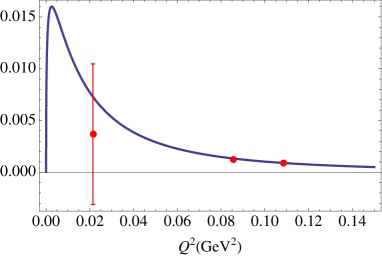
Fig. 1 shows the integrand of Eq. (1) in the low-$Q^{2}$ region; it is peaked around $Q^{2}\sim m_{\mu}^{2}/4$. The points with error bars show typical lattice data for this integrand.[5] The lattice data are restricted to values of $Q^{2}$ available with periodic boundary conditions in finite volume. The figure demonstrates an important problem in obtaining HVP from the lattice: to obtain lattice data near the peak of the integrand, lattices with a linear volume $2\pi/L\sim m_{\mu}/2$, i.e., $L\sim 25$ fm would be needed! With a lattice spacing $a$ of order $0.06$ fm necessary in order to reach the continuum limit, this would imply $L/a\sim 400$, clearly out of reach given present computational resources.

There are two ways in which one might proceed in order to make progress. One method is clearly to obtain more data at smaller $Q^{2}$. If one makes use of twisted instead of periodic boundary conditions, one can in principle reach smaller $Q^{2}$ values without increasing the size of the lattice. Investigations in this direction are in progress.[6] The other is to obtain more precise data at currently available values of $Q^{2}$, using for instance AMA error reduction.[7] If a theoretically reliable fit function for the $Q^{2}$ behavior of $\Pi(Q^{2})$ can be found, it may then be possible to extrapolate the integrand of Eq. (1) to smaller values of $Q^{2}$, so that the integral $a_{\mu}^{\rm HVP}$ can be computed with a small enough error. Quite likely, a combination of these methods will be necessary in practice.

The most commonly used fitting functions are based on the assumption of vector meson dominance (VMD).[8] The problem with these is that such fits assume that the lowest singularity in $\Pi(Q^{2})$ is at $-Q^{2}=m_{\rho}^{2}$, while in reality $\Pi(Q^{2})$ has a cut starting at $-Q^{2}=4m_{\pi}^{2}\ll m_{\rho}^{2}$. Clearly, the use of this assumption introduces a model element into the computation, in conflict with the notion of the lattice providing us with an approach from first principles!

Theoretically, one can do much better. Based on results obtained in the literature on Padé approximants (PAs), it was proven in Ref. ABGP2012 that the functions

$$\Pi(Q^{2})=\Pi(0)-Q^{2}\left(a_{0}+\sum_{n=1}^{[P/2]}\frac{a_{n}}{b_{n}+Q^{2}}\right)\ ,\quad a_{n\geq 1}>0\ ,\quad b_{n}\geq 4m_{\pi}^{2}$$ (2)

with either $a_{0}=0$ or $a_{0}$ free provide a series of PAs converging to the vacuum polarization everywhere except near the cut $Q^{2}\in(-\infty,-4m_{\pi}^{2}]$ on the Minkowski axis. We note that choosing $P=2$, $a_{0}=0$ and $b_{1}=m_{\rho}^{2}$ corresponds to a VMD-type assumption, but it does not correspond to a valid PA: as we increase the order of the PA, the poles in Eq. (2) should approach the branch point at $Q^{2}=-4m_{\pi}^{2}$.

While initial explorations of the PA-based fitting method of the low-$Q^{2}$ behavior of $\Pi(Q^{2})$ look promising,[5] it is important to have an independent test of any fitting method. This is particularly important as long as the data in the strongly peaked region of Fig. 1 will remain sparse. Reference GMP2013 describes the construction of a QCD-based model that allows us to set up a “test laboratory” for fits of the low-$Q^{2}$ behavior of $\Pi(Q^{2})$. This model combines the non-strange vector $\tau$ spectral data with a quantitative description beyond the $\tau$ mass using perturbation theory and a model for duality violations in order to create a model for $\Pi(Q^{2})$ using a dispersion relation. In this model, the “exact” value of the integral below $1$ GeV² is

$$\tilde{a}_{\mu}^{\mbox{HVP},Q^{2}\leq 1~{}\mbox{GeV}^{2}}=1.204\times 10^{-7}\ ,$$ (3)

where the tilde reminds us that this quantity is not $a_{\mu}$ itself, but instead corresponds to twice the $I=1$ part below 1 GeV². Using a covariance matrix for $\Pi(Q^{2})$ data points obtained from a lattice computation, we may now use the model in order to create realistically correlated fake data sets at typical lattice values of the momenta $Q^{2}$. These data sets can then be fitted using VMD- or PA-type fit functions, allowing us to compare fitted values for $\tilde{a}_{\mu}^{\mbox{HVP},Q^{2}\leq 1~{}\mbox{GeV}^{2}}$ with the exact value in Eq. (3).

Various correlated fits of the “lattice” data set on the interval $0<Q^{2}\leq 1$ GeV². Fit $\tilde{a}_{\mu}\times 10^{7}$ error $\times 10^{7}$ pull $\chi^{2}/\mbox{dof}$ VMD 1.3201 0.0052 22 2189/47 VMD$+$ 1.0658 0.0076 18 67.4/46 PA $[0,1]$ 0.8703 0.0095 35 285/46 PA $[1,1]$ 1.116 0.022 4 61.4/45 PA $[1,2]$ 1.182 0.043 0.5 55.0/44 PA $[2,2]$ 1.177 0.058 0.5 54.6/43

Results for such fits are shown in Table THE MUON ANOMALOUS MAGNETIC MOMENT, A VIEW FROM THE LATTICE . VMD$+$ corresponds to VMD plus a linear term, and the PA fits correspond to Eq. (2) with $P\geq 2$, $a_{0}=0$ or $a_{0}$ free. For details, we refer to Ref. GMP2013. The first column lists the type of fit, the second column gives the value of $\tilde{a}_{\mu}^{\mbox{HVP},Q^{2}\leq 1~{}\mbox{GeV}^{2}}$ from the fit, the third column the error from the fit, and the fifth column the value of $\chi^{2}$ per degree of freedom for the fit. From the $\chi^{2}$ values, one would conclude the VMD$+$ fit to be reasonable, and one would accept the PA fits $[1,1]$, $[1,2]$ and $[2,2]$, if no extra information were available.

However, in our model tests, we can compare the fitted value with the exact value. The fourth column shows the “pull,” defined by

$$\mbox{pull}=\frac{|\mbox{exact~{}value}-\mbox{fitted~{}value}|}{\mbox{fit~{}error}}\ .$$ (4)

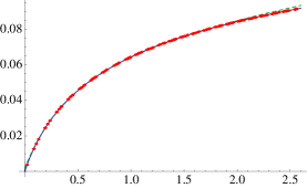
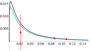
From its values, we see that both VMD-type fits are very bad fits; there is a large discrepancy between the precision as measured by the fit error and the accuracy as measured by the pull (even though the VMD$+$ fit has an acceptable $\chi^{2}/$dof). Also the $[1,1]$ PA is not very good — only the higher order PAs yield good fits, but the fit error is of order 5%. For illustration, we show the VMD$+$ fit in Fig. 2. While the $\Pi(Q^{2})$ fit looks very good, this is not the case for the integrand of Eq. (1). A similar figure for the $[1,2]$ PA looks much better.[9]

Figure 2: VMD$+$ fit: green dashed curves; model: blue solid curves. Left panel: vacuum polarization; right panel: integrand of Eq. (1) for low $Q^{2}$; red points are “lattice” data points. Units as in Fig. 1.

In conclusion, we believe that it is important to pursue $a_{\mu}^{\rm HVP}$ using Lattice QCD, but it is clear that much work remains in order to ascertain the accuracy with which this can be done. In particular, we advocate the use of fit functions for the low-$Q^{2}$ behavior of $\Pi(Q^{2})$ based on known convergence properties, and the use of detailed tests as sketched above in order to test fit strategies as part of the error analysis of any determination of $a_{\mu}^{\rm HVP}$ from the lattice.

References

- [1] J. P. Miller, E. de Rafael and B. L. Roberts, Rept. Prog. Phys. 70, 795 (2007) [hep-ph/0703049]; F. Jegerlehner and A. Nyffeler, Phys. Rept. 477, 1 (2009) [arXiv:0902.3360 [hep-ph]].
- [2] For a recent review of lattice efforts, see T. Blum, M. Hayakawa and T. Izubuchi, PoS LATTICE 2012, 022 (2012) [arXiv:1301.2607 [hep-lat]].
- [3] F. Jegerlehner and R. Szafron, Eur. Phys. J. C 71, 1632 (2011) [arXiv:1101.2872 [hep-ph]].
- [4] T. Blum, Phys. Rev. Lett. 91, 052001 (2003) [hep-lat/0212018]; B. E. Lautrup et al., Phys. Rept. 3, 193 (1972).
- [5] C. Aubin et al., Phys. Rev. D 86, 054509 (2012) [arXiv:1205.3695 [hep-lat]].
- [6] M. Della Morte et al., JHEP 1203, 055 (2012) [arXiv:1112.2894 [hep-lat]]; PoS LATTICE 2012, 175 (2012) [arXiv:1211.1159 [hep-lat]]; C. Aubin et al., Phys. Rev. D 88, 074505 (2013) [arXiv:1307.4701 [hep-lat]].
- [7] T. Blum, T. Izubuchi and E. Shintani, Phys. Rev. D 88, 094503 (2013) [arXiv:1208.4349 [hep-lat], arXiv:1208.4349 [hep-lat]].
- [8] C. Aubin and T. Blum, Phys. Rev. D 75, 114502 (2007) [arXiv:hep-lat/0608011]; X. Feng et al., Phys. Rev. Lett. 107, 081802 (2011) [arXiv:1103.4818 [hep-lat]]; PoS LATTICE 2012, 174 (2012) [arXiv:1211.0828 [hep-lat]]; P. Boyle et al., arXiv:1107.1497 [hep-lat].
- [9] M. Golterman, K. Maltman and S. Peris, arXiv:1309.2153 [hep-lat].