Multifractals, Mumford curves, and Eternal Inflation

Abstract.

We relate the Eternal Symmetree model of Harlow, Shenker, Stanford, and Susskind to constructions of stochastic processes related to quantum statistical mechanical systems on Cuntz–Krieger algebras. We extend the eternal inflation model from the Bruhat–Tits tree to quotients by $p$-adic Schottky groups, again using quantum statistical mechanics on graph algebras.

1. Introduction

A model of eternal inflation based on a tree structure was developed recently by Harlow, Shenker, Stanford, and Susskind, see [9] and [19], based on $p$-adic Bruhat–Tits trees.

We revisit the model here from the point of view of fractal geometry and noncommutative geometry, using constructions of stochastic processes, multifractal measures and wavelets, associated to Cuntz and Cuntz–Krieger algebras, [14], [16], as well as a operator algebraic methods applied to the geometry of $p$-adic Mumford curves, as previously developed in [4].

In particular, we show that the type of stochastic process considered in the eternal inflation model of [9], in the case of a particular class of “pruning methods” associated to subshifts of finite type, can be obtained from the KMS equilibrium states of a quantum statistical mechanical system on a noncommutative operator algebra associated to the pruned tree. In particular this implies that what plays the role of the proper time in the model, which gives the discrete evolution of the stochastic process, in turn can be seen as depending on an internal notion of time evolution acting on the creation and annihilation operators given by the generators of the noncommutative algebra associated to the graph. The propagators in the correlation functions for the multiverse fields of [9] in turn provide a measure of autocorrelation for wavelets on fractals arising from the construction of the multifractal measure (as in [7], [16]) on the boundary of the tree, which determined the stochastic process.

We also show how one can extend the eternal inflation model from the case of the $p$-adic Bruhat–Tits tree to infinite graphs given by quotients of the Bruhat–Tits tree by a $p$-adic Schottky group. These graphs have boundary at infinity given by a $p$-adically uniformized Mumford curve, and they consist of a central finite graph (the dual graph of the closed fiber of the minimal smooth model of the curve) with infinite trees sticking out of its vertices. We show that one can consistently interpolate random processes on the external trees of the type considered in [9] to a stochastic process on the entire graph, which is constructed using KMS weights of an associated graph $C^{*}$-algebra. The picture that emerges is one where the dynamics of the eternal inflation model can remain trapped inside a bounded region given by the finite graph, or wander off into one of the trees, where it reproduces the model of [9].

2. The Eternal Symmetree model

The Eternal Symmetree of [9] is a discretized model of eternal inflation. In this model, a multiverse landscape arises through a stochastic process describing the likelihood of transitions between different types of vacua, labeled by the letters of a finite alphabet ${\mathfrak{A}}=\{0,\ldots,p-1\}$. Each vacuum represents a collection of microstates with assigned entropies $S=(S_{a})_{a\in{\mathfrak{A}}}$.

The causal future of a node in the tree is the oriented subtree that branches off from that node to the boundary at infinity. Time is discretized, with the proper time between two adjacent nodes being given by a fixed amount, the inverse of the Hubble constant, which can vary with the label attached to the edge.

A collection of multiverse fields is described in [9], with correlation functions expressed in terms of the data of the stochastic process and of the $p$-adic distance on the Bruhat–Tits tree. The group ${\rm PGL}_{2}({\mathbb{Q}}_{p})$ of isometries of the Bruhat–Tits tree of ${\mathbb{Q}}_{p}$ acts as conformal symmetries. The symmetry is broken if the tree is suitably “pruned”, giving rise to terminal vacua. This alters the form of the the correlation functions, leading to the emergence of a “fractal-flow” arrow-of-time, see [19].

We first describe how to reinterpret the case without terminal vacua in terms of multifractal measures and operator algebra arising from representations of the Cuntz algebras of [5]. We show, in particular, that the construction of the multiverse fields in the Eternal Symmetree model is closely related to the construction of [7] (see also [14]) of stochastic processes and wavelets on the Cantor sets dual to the maximal abelian subalgebra of the Cuntz algebra.

We will then consider the case with terminal vacua, where we focus on pruning of the tree obtained through an admissibility condition on adjacent edges. We will show that the model can be reinterpreted as passing from Cuntz algebras to Cuntz–Krieger algebra, where once again one can relate the multiverse fields to stochastic processes, multifractal measures and wavelets on the associated Cantor sets, as in [16].

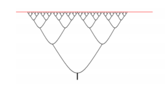
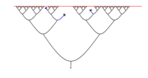
Figure 1. The Eternal Symmetree without and with pruning, as illustrated in [9].

2.1. Bruhat–Tits trees

Let ${\mathcal{T}}$ be a uniform infinite tree with vertices of valence $q+1$, with $q\geq 2$. We are interested in particular in the case where ${\mathcal{T}}$ is the Bruhat–Tits tree of ${\rm PGL}_{2}({\mathbb{K}})$, with ${\mathbb{K}}$ a finite extension of ${\mathbb{Q}}_{p}$. In this case the integer $q=p^{r}$ is the cardinality of the residue field of ${\mathbb{K}}$. A ray is a half-infinite path without backtracking and an infinite geodesic is an infinite path without backtracking. We denote by $\partial{\mathcal{T}}$ the boundary at infinity of the tree, which is the set of equivalence classes of rays, where two rays are equivalent if they have an infinite number of vertices in common. Any choice of two distinct points on the boundary determines a unique infinite geodesic in ${\mathcal{T}}$ that connects them. In the case of the Bruhat–Tits tree, the boundary is identified with ${\mathbb{P}}^{1}({\mathbb{K}})$. We refer the reader to [8], [13], [17] for a detailed exposition of the $p$-adic geometry of Bruhat–Tits trees and their quotients.

The choice of a coordinate function $z$ on ${\mathbb{P}}^{1}({\mathbb{K}})=\partial{\mathcal{T}}$ corresponds to fixing the choice of points $\{0,1,\infty\}$ in ${\mathbb{P}}^{1}({\mathbb{K}})$. This in turn determines a unique choice of a vertex $v_{0}$ of the tree ${\mathcal{T}}$, as the unique origin of three non-overlapping rays with endpoints $\{0,1,\infty\}$. Let $v_{0}$ be a the base vertex in the tree ${\mathcal{T}}$ obtained in this way. We choose an orientation of the tree ${\mathcal{T}}$ with all the edges pointing outwards from $v_{0}$, so that at each vertex $v\neq v_{0}$ we have one incoming and $q$ outgoing edges.

In particular, having fixed a projective coordinate on ${\mathbb{P}}^{1}({\mathbb{K}})$ and a corresponding base vertex in ${\mathcal{T}}$ we have a subtree ${\mathcal{T}}^{\prime}$ of the Bruhat–Tits tree ${\mathcal{T}}$, with root $v_{0}$, whose boundary $\partial{\mathcal{T}}^{\prime}={\mathcal{O}}_{{\mathbb{K}}}$ consists of the integers of ${\mathbb{K}}$, the $p$-adic integers ${\mathbb{Z}}_{p}$ in the case where ${\mathbb{K}}={\mathbb{Q}}_{p}$. This is the tree considered in the Eternal Symmetree model of [9], [19], where the subtree ${\mathcal{T}}^{\prime}$ of the Bruhat–Tits tree is referred to as the Bethe tree.

This admits an equivalent description in terms of $\omega$-languages, which will be useful in the following.

2.2. $\omega$-languages

Suppose given a finite alphabet ${\mathfrak{A}}$ with $\#{\mathfrak{A}}=q$ with $q\geq 2$. Let ${\mathcal{W}}_{{\mathfrak{A}}}$ denote the union ${\mathcal{W}}_{{\mathfrak{A}}}^{\star}=\cup_{k=0}^{\infty}{\mathcal{W}}_{{\mathfrak{A}},k}$ of the sets ${\mathcal{W}}_{{\mathfrak{A}},k}$ of length $k$ in the alphabet ${\mathfrak{A}}$. For $k=0$, ${\mathcal{W}}_{{\mathfrak{A}},0}$ consists of the empty word $\epsilon=\emptyset$. We denote by ${\mathcal{W}}_{\mathfrak{A}}^{\omega}$ the set of all infinite words $a=a_{0}a_{1}\cdots a_{n}\cdots$ with $a_{k}\in{\mathfrak{A}}$. A language ${\mathcal{L}}$ is a subset of ${\mathcal{W}}_{{\mathfrak{A}}}^{\star}$ and an $\omega$-language ${\mathcal{L}}^{\omega}$ is a subset of ${\mathcal{W}}_{{\mathfrak{A}}}^{\omega}$.

The shift operator $\sigma:{\mathcal{W}}_{{\mathfrak{A}}}^{\omega}\to{\mathcal{W}}_{{\mathfrak{A}}}^{\omega}$ is defined as the map $\sigma:a_{0}a_{1}\cdots a_{n}\cdots\mapsto a_{1}a_{2}\cdots a_{n+1}\cdots$ that shifts the sequence one step to the left and drops the first letter. We require that the $\omega$-languages ${\mathcal{L}}^{\omega}$ we consider are shift-invariant, in the sense that if an infinite word $a\in{\mathcal{W}}_{{\mathfrak{A}}}^{\omega}$ is in ${\mathcal{L}}^{\omega}$, then its shifted image $\sigma(a)$ is also in ${\mathcal{L}}^{\omega}$.

2.3. Subshifts of finite type

We consider in particular $\omega$-languages that are obtained by imposing an admissibility condition on successive letters in infinite words in ${\mathcal{W}}_{{\mathfrak{A}}}^{\omega}$. These have the properties of being shift-invariant. In terms of the dynamical system defined by the shift map, they correspond to subshifts of finite type.

These are determined by assigning an admissibility matrix $A=(A_{ab})_{a,b\in{\mathfrak{A}}}$ with entries in $\{0,1\}$. The corresponding $\omega$-languages ${\mathcal{L}}_{A}^{\omega}$ consists of admissible infinite words in ${\mathcal{W}}_{{\mathfrak{A}}}^{\omega}$, namely those infinite where subsequent letters satisfy the condition that the corresponding entry of the matrix $A$ is non-zero,

$${\mathcal{L}}_{A}^{\omega}=\{a_{0}a_{1}\cdots a_{n}\cdots\,|\,A_{a_{k}a_{k+1}}=1,\,\forall k\geq 0\}.$$

Both the space of infinite words ${\mathcal{W}}_{{\mathfrak{A}}}^{\omega}$ and the subspace ${\mathcal{L}}_{A}^{\omega}$ can be topologized as Cantor sets, with a basis of clopen sets given by the cylinders $\Lambda(w)$, where $\Lambda$ is either ${\mathcal{W}}_{{\mathfrak{A}}}^{\omega}$ or ${\mathcal{L}}_{A}^{\omega}$. These are the sets of all infinite words in $\Lambda$ that start with an assigned (admissible) word $w$ of finite length. The shift map $\sigma$ is a continuous dynamical system with respect to this topology.

2.4. Terminal vacua and subshifts of finite type

Let ${\mathcal{T}}^{\prime}\subset{\mathcal{T}}$ be the Bethe tree, that is, the rooted tree with $\partial{\mathcal{T}}^{\prime}={\mathcal{O}}_{{\mathbb{K}}}$, as above.

Lemma 2.1.

The boundary at infinity $\partial{\mathcal{T}}^{\prime}$ of the Bethe tree ${\mathcal{T}}^{\prime}$ can be equivalently described as the Cantor set of infinite words ${\mathcal{W}}_{{\mathfrak{A}}}^{\omega}$ in an alphabet ${\mathfrak{A}}={\mathbb{F}}_{q}$, identified (as a set) with the residue field of ${\mathbb{K}}$.

Proof.

For simplicity, we look at the case ${\mathbb{K}}={\mathbb{Q}}_{p}$. The case of finite extensions is analogous. The $p$-adic integers in ${\mathbb{Z}}_{p}$ can be written as infinite series $x=\sum_{k=0}^{\infty}x_{k}p^{k}$, in powers of $p$, with coefficients in $\{0,\ldots,p-1\}$. This corresponds to labeling the outgoing edges at each vertex of ${\mathcal{T}}^{\prime}$ with a set of labels $\{e_{i}\}_{i=0,\ldots,p-1}$. Thus, one can identify rays starting at $v_{0}$ with arbitrary infinite words in the alphabet ${\mathfrak{A}}=\{e_{i}\}_{i=0,\ldots,p-1}$. ∎

The action of the shift operator is related to the notion of proper time in the Eternal Symmetree model, which corresponds to the discretized movement towards one of the next adjacent nodes in the forward direction along the tree.

We see then that introducing an admissibility condition $A=(A_{ab})$ as above corresponds to a way of pruning the tree ${\mathcal{T}}^{\prime}$. Namely, any ray of ${\mathcal{T}}^{\prime}$ that contains a non-admissible consecutive pair of edges $e_{k}e_{k+1}$ is removed from the tree, by cutting the branch at the place where the first non-admissible pair occurs, coming out of the root. This provides a mechanism that creates terminal vacua.

In the Eternal Symmetree model, more general mechanisms for pruning the tree ${\mathcal{T}}^{\prime}$ are considered, which do not necessarily correspond to admissibility conditions defined by a matrix $A$. These other pruning methods will give rise to more general kinds of $\omega$-languages, which are not necessarily shift invariant. We focus here only on pruning defined by admissibility conditions determined by a matrix $A$, as these will be directly related to an important class of operator algebras, as we show in the following section.

3. Multifractal measures via quantum statistical mechanics

In this section we reinterpret the stochastic process of the Eternal Symmetree model in terms of multifractal measures related to representations of Cuntz–Krieger algebras.

3.1. Entropies and stochastic processes on the Eternal Symmetree

In the eternal inflation model of [9], the letters of the alphabet ${\mathfrak{A}}$ correspond to “color” labels for the different types of vacua, with each color corresponding to a collection of microstates. These have associated entropies given by a collection $\{S_{a}\}_{a\in{\mathfrak{A}}}$. At each node there are probabilities $\gamma_{ab}$ of transition from an incoming color $a$ to an outgoing color $b$. These measure the probability of tunneling between vacua of different types. A detailed balance condition of microscopic reversibility is imposed on the probabilities $\gamma_{ab}$, of the form

(3.1) $$\frac{\gamma_{ab}}{\gamma_{ba}}=e^{S_{a}-S_{b}}.$$

The detailed balance condition is expressed in [9] through a real symmetric matrix $M$ such that $\gamma_{ab}=M_{ab}e^{S_{a}}$.

In the case without terminal vacua, a stochastic process is constructed out of these data, with $P_{a}(k)$ the probability of obtaining a vacuum of type $a\in{\mathfrak{A}}$ after $k$ steps from the root vertex in ${\mathcal{T}}^{\prime}$. These probabilities are written as $P_{a}=e^{S_{a}/2}\Phi_{a}$, with the $\Phi_{a}$ satisfying the process

(3.2) $$\Phi(k+1)={\mathcal{S}}\,\Phi(k),$$

where ${\mathcal{S}}$ is a positive stochastic matrix with Perron–Frobenius eigenvalue $\lambda_{{\mathcal{S}}}=1$ and positive Perron–Frobenius eigenvector $v_{{\mathcal{S}}}$.

In [9] the matrix $\gamma_{ab}$ is in turn related to the matrix ${\mathcal{S}}_{ab}$ by ${\mathcal{S}}=Z^{-1}GZ$ with $Z$ the diagonal matrix with entries $e^{S_{a}/2}$ and with $G_{ab}=\delta_{ab}-\sum_{c}\gamma_{ca}\delta_{ab}+\gamma_{ab}$.

We will now reinterpret this construction in terms of stochastic processes related to Cuntz algebras.

3.2. Potentials with the Keane condition

On the Cantor set $\Lambda={\mathcal{W}}_{\mathfrak{A}}^{\omega}$, we consider ${\mathbb{R}}_{+}$-valued potentials $W_{\beta}$ satisfying the Keane condition:

(3.3) $$\sum_{a\in{\mathfrak{A}}}W_{\beta}(ax)=1,\ \ \ \forall x\in{\mathcal{W}}_{\mathfrak{A}}^{\omega}.$$

This condition has a direct interpretation in terms of Ruelle transfer operators

$${\mathcal{R}}_{\sigma,W,\beta}\,f(x)=\sum_{\sigma(y)=x}W_{\beta}(y)f(y)=\sum_{a\in{\mathfrak{A}}}W_{\beta}(ax)\,f(ax).$$

Namely, the Keane condition implies that $f(x)\equiv 1$ is fixed point of ${\mathcal{R}}_{\sigma,W,\beta}$.

The choice of a Keane potential $W_{\beta}$ on $\Lambda$ gives rise to a multifractal measure on $\Lambda$ obtained as a stochastic process as follows. Choose a base point $x_{0}\in{\mathcal{W}}_{\mathfrak{A}}^{\omega}$, and define the measure $\mu_{W,\beta,x_{0}}$ by setting

(3.4) $$\mu_{W,\beta,x_{0}}(\Lambda(w))=W_{\beta}(a_{1}x_{0})W_{\beta}(a_{2}a_{1}x_{0})\cdots W_{\beta}(a_{m}\cdots a_{2}a_{1}x_{0})$$

for $w=a_{0}\cdots a_{m}\in{\mathcal{W}}_{{\mathfrak{A}},m}$ and

$$\Lambda(w)=\{a\in{\mathcal{W}}_{\mathfrak{A}}^{\omega}\,|\,a_{0}\cdots a_{m}=w\}.$$

The Keane condition ensures that (3.4) indeed defines a measure, see [7], [16].

We focus in particular on two examples of potentials $W_{\beta}$, already considered in [14] in relation to coding theory. The first example gives a stochastic process governed by a Bernoulli measure and the second one by a Markov measure.

Example 3.1.

For $x=x_{1}x_{2}x_{3}\cdots x_{n}\cdots\in\Lambda$, set $W_{\beta}(x)=e^{-\beta\lambda_{x_{1}}}$, where the weights $\{\lambda_{a}\}_{a\in{\mathfrak{A}}}$ satisfy

$$\sum_{a\in{\mathfrak{A}}}e^{-\beta\lambda_{a}}=1.$$

Then the multifractal measure on $\Lambda$ is given by

$$\mu_{W,\beta,x}(\Lambda(w))=\prod_{j=0}^{m}e^{-\beta\lambda_{w_{j}}},$$

for $w=w_{1}w_{2}\cdots w_{m}\in{\mathcal{W}}_{{\mathfrak{A}},m}$, and $w_{0}=x_{1}$.

Example 3.2.

For $x=x_{1}x_{2}x_{3}\cdots x_{n}\cdots\in\Lambda$, set $W_{\beta}(x)=e^{-\beta\lambda_{x_{1}x_{2}}}$, where the matrix $(\lambda_{ab})_{a,b\in{\mathfrak{A}}}$ satisfies the stochastic condition

$$\sum_{a\in{\mathfrak{A}}}e^{-\beta\lambda_{ab}}=1,\ \ \forall b\in{\mathfrak{A}}.$$

Then the measure is given by

$$\mu_{W,\beta,x}(\Lambda(w))=e^{-\beta\lambda_{w_{m}w_{m-1}}}\cdots e^{-\beta\lambda_{w_{2}w_{1}}}e^{-\beta\lambda_{w_{1}x_{1}}}.$$

We will see how to adapt the second example to match the required properties for a stochastic process on the Eternal Symmetree.

3.3. Cuntz algebras

Stochastic processes of the type (3.4) were considered as a source of wavelet constructions in [7], and related to representations of Cuntz algebras.

Given a finite set ${\mathfrak{A}}$, the Cuntz algebra ${\mathcal{O}}_{\mathfrak{A}}$ is the universal $C^{*}$-algebra generated by isometries $S_{a}$ with $a\in{\mathfrak{A}}$ with the relation

$$\sum_{a\in{\mathfrak{A}}}S_{a}S_{a}^{*}=1$$

and $S^{*}_{a}S_{b}=\delta_{a,b}$.

The maximal abelian subalgebra of ${\mathcal{O}}_{\mathfrak{A}}$ is generated by the projections $P_{w}=S_{w}S_{w}^{*}$ with $w\in{\mathcal{W}}_{{\mathfrak{A}}}^{\star}$. It is isomorphic to the $C^{*}$-algebra of continuous functions $C(\Lambda_{{\mathfrak{A}}})$ on a Cantor set $\Lambda_{{\mathfrak{A}}}={\mathcal{W}}_{{\mathfrak{A}}}^{\omega}$. For more details on the properties of Cuntz algebras, we refer the reader to [5].

We will discuss in detail the relation of Cuntz algebras to the multifractal measures $\Lambda_{{\mathfrak{A}}}$ and stochastic processes arising from potentials with the Keane conditions in §3.7 below, in the more general case of Cuntz–Krieger algebras.

3.4. Multifractal measures and stochastics on the Eternal Symmetree

We now show that a stochastic process $P_{a}=e^{S_{a}/2}\Phi_{a}$ satisfying (3.2) on the Eternal Symmetree without pruning can be obtained as the multifractal measure determined by a particular choice of Keane potential on the Cantor set $\Lambda_{{\mathfrak{A}}}$.

Proposition 3.3.

Let ${\mathcal{S}}=({\mathcal{S}}_{ab})$ be a symmetric positive stochastic matrix with Perron–Frobenius eigenvalue $\lambda_{\mathcal{S}}=1$ and positive (left) Perron–Frobenius eigenvector $v_{{\mathcal{S}}}$, normalized by $\sum_{a\in{\mathfrak{A}}}v_{{\mathcal{S}},a}=1$. Then

(3.5) $$W(x)=v_{{\mathcal{S}},x_{1}}\,{\mathcal{S}}_{x_{1},x_{2}}\,v_{{\mathcal{S}},x_{2}}^{-1}$$

defines a potential on $\Lambda_{{\mathfrak{A}}}$ satisfying the Keane condition. The multifractal measure $\mu_{W,x}$ on $\Lambda_{{\mathfrak{A}}}$ determined by $W$ and the choice of a base point $x$ defines a stochastic process $\Phi_{x,a}(m)$ on the Eternal Symmetree without pruning, satisfying (3.2).

Proof.

The potential (3.5) satisfies the Keane condition (3.3), since we have

$$\sum_{a\in{\mathfrak{A}}}W(ax)=\sum_{a\in{\mathfrak{A}}}v_{{\mathcal{S}},a}\,{\mathcal{S}}_{a,x_{1}}\,v_{{\mathcal{S}},x_{1}}^{-1}=v_{{\mathcal{S}},x_{1}}\,v_{{\mathcal{S}},x_{1}}^{-1}=1,$$

by the Perron–Frobenius condition. We interpret the coordinates of the Perron–Frobenius eigenvector $v_{{\mathcal{S}}}$ in terms of the entropies of the Symmetree model, by setting $v_{{\mathcal{S}},a}=e^{-S_{a}/2}$. The resulting multifractal measure $\mu_{W,x}$ is then given by

$$\mu_{W,x}(\Lambda(w))=e^{(S_{x_{1}}-S_{w_{m}})/2}{\mathcal{S}}_{w_{m}w_{m-1}}\cdots{\mathcal{S}}_{w_{2}w_{1}}{\mathcal{S}}_{w_{1},x_{1}},$$

for a choice of an endpoint $x\in\Lambda_{{\mathfrak{A}}}$ and of a finite word $w=w_{m}w_{m-1}\cdots w_{1}$ in ${\mathcal{W}}^{\star}_{\mathfrak{A}}$. Setting $\Phi_{x,a}(m+1)=e^{S_{a}/2}\sum_{w}\mu_{W,x}(\Lambda(aw))$, we obtain

$$\mu_{W,x}(\Lambda(aw))=e^{(S_{x_{1}}-S_{a})/2}{\mathcal{S}}_{aw_{m}}{\mathcal{S}}_{w_{m}w_{m-1}}\cdots{\mathcal{S}}_{w_{2}w_{1}}{\mathcal{S}}_{w_{1},x_{1}}.$$

This satisfies

$$\sum_{w}\mu_{W,x}(\Lambda(aw))=e^{(S_{x_{1}}-S_{a})/2}\sum_{w}{\mathcal{S}}_{aw_{m}}{\mathcal{S}}_{w_{m}w_{m-1}}\cdots{\mathcal{S}}_{w_{2}w_{1}}{\mathcal{S}}_{w_{1},x_{1}}=e^{(S_{x_{1}}-S_{a})/2}{\mathcal{S}}^{m}_{a,x_{1}}.$$

Thus, we obtain that $\Phi_{x,a}(m+1)=e^{S_{a}/2}\sum_{w}\mu_{W,x}(\Lambda(aw))$ satisfies (3.2), since

$$\Phi_{x,a}(m+1)=e^{S_{x_{1}}/2}{\mathcal{S}}^{m}_{a,x_{1}}=e^{S_{x_{1}}/2}\sum_{b}{\mathcal{S}}_{a,b}{\mathcal{S}}^{m-1}_{b,x_{1}}=\sum_{b}{\mathcal{S}}_{a,b}\Phi_{x,b}(m).$$

∎

Remark 3.4.

The dependence on the choice of a basepoint $x\in\Lambda_{\mathfrak{A}}$ of the random process $\Phi_{x,a}(m)$ constructed in Proposition 3.3 can be averaged out by setting

(3.6) $$\Phi_{a}(m)=\int_{\Lambda_{{\mathfrak{A}}}}\Phi_{x,a}(m)\,d\mu(x),$$

with $\mu$ the normalized Hausdorff measure on the Cantor set $\Lambda_{{\mathfrak{A}}}$. This still satisfies $\Phi(m+1)={\mathcal{S}}\,\Phi(m)$.

It is convenient for our purposes, to rewrite the potential $W$ of (3.5) and the resulting stochastic process in terms of an auxiliary parameter $\beta$, which will play the role of a thermodynamic parameter when we reintepret the construction as arising from a quantum statistical mechanical system.

Corollary 3.5.

For a given $\beta>0$, the potential (3.5) can be obtained as a particular case of Example 3.2 with

(3.7) $$W_{\beta}(x)=e^{-\beta\lambda_{x_{1}x_{2}}}=e^{-\beta\lambda_{x_{1}}}\,{\mathcal{S}}_{x_{1}x_{2}}\,e^{\beta\lambda_{x_{2}}},$$

with ${\mathcal{S}}=(S_{ab})_{a,b\in{\mathfrak{A}}}$ a symmetric positive stochastic matrix as in Proposition 3.3 and with the weights $\lambda_{a}$ chosen so that

(3.8) $$e^{-\beta\lambda_{a}}=(v_{S})_{a}=e^{-S_{a}/2},$$

where, as above, $v_{\mathcal{S}}$ is the (left) Perron-Frobenius eigenvector, normalized by

(3.9) $$\sum_{a\in{\mathfrak{A}}}e^{-\beta\lambda_{a}}=1.$$

The resulting multifractal measure, in the notation of Corollary 3.5, is given by

(3.10) $$\mu_{W,\beta,x}(\Lambda(w))=e^{-\beta\lambda_{w_{m}w_{m-1}}}\cdots e^{-\beta\lambda_{w_{2}w_{1}}}e^{-\beta\lambda_{w_{1}x_{1}}}=e^{\beta(\lambda_{x_{1}}-\lambda_{w_{m}})}{\mathcal{S}}_{w_{m}w_{m-1}}\cdots{\mathcal{S}}_{w_{2}w_{1}}{\mathcal{S}}_{w_{1},x_{1}}.$$

Corollary 3.6.

Let $e^{-\tilde{S}_{a}/2}=\tilde{v}_{{\mathcal{S}},a}$, with $\tilde{v}_{\mathcal{S}}$ a (right) Perron-Frobenius eigenvector for ${\mathcal{S}}$. Setting $P_{a}(m)=e^{-\tilde{S}_{a}/2}/{\mathcal{N}}$ with ${\mathcal{N}}=\sum_{a}e^{-\tilde{S}_{a}/2}$ gives a stationary process satisfying $P_{a}(m+1)=\sum_{b}S_{ab}P_{b}(m)$ and $P_{a}(m+1)=P_{a}(m)$.

Proof.

Since $e^{-\tilde{S}_{a}/2}=\tilde{v}_{{\mathcal{S}},a}$ is a (right) Perron–Frobenius eigenvector of ${\mathcal{S}}$ with $\lambda_{{\mathcal{S}}}=1$, we have $P_{a}(m+1)=\sum_{b}S_{ab}P_{b}(m)=\sum_{b}S_{ab}e^{-\tilde{S}_{a}/2}/{\mathcal{N}}=e^{-\tilde{S}_{b}/2}/{\mathcal{N}}=P_{a}(m)$. ∎

3.5. Terminal vacua via Cuntz–Krieger algebras

Let ${\mathfrak{A}}$ be a finite set and let $A=(A_{ab})_{a,b\in{\mathfrak{A}}}$ be a matrix with entries $A_{a,b}\in\{0,1\}$. We use the matrix $A$ as a way of pruning the Bethe tree. The analog of the Cuntz algebra in the case of a subshift of finite type with admissibility condition given by $A$ is given by the Cuntz–Krieger algebra ${\mathcal{O}}_{{\mathfrak{A}},A}$, see [6].

The Cuntz–Krieger algebra ${\mathcal{O}}_{{\mathfrak{A}},A}$ is the universal $C^{*}$-algebra generated by partial isometries $S_{a}$ with $a\in{\mathfrak{A}}$, with relations

$$S_{a}^{*}S_{a}=\sum_{b}A_{ab}\,S_{b}S_{b}^{*},$$

$$\sum_{a\in{\mathfrak{A}}}S_{a}S_{a}^{*}=1.$$

The Cuntz algebras recalled above correspond to the special case where the matrix $A$ has all entries equal to one, that is, to the unpruned case.

The maximal abelian subalgebra of ${\mathcal{O}}_{{\mathfrak{A}},A}$ is generated by the projections $S_{w}S_{w}^{*}$, with $w\in{\mathcal{W}}^{\star}_{{\mathfrak{A}},A}$ words with admissibility condition $A_{w_{k},w_{k+1}}=1$, in the language ${\mathcal{L}}_{A}$. It is isomorphic to the $C^{*}$-algebra $C(\Lambda_{{\mathfrak{A}},A})$ of continuous functions on the Cantor set $\Lambda_{{\mathfrak{A}},A}$. This is the set ${\mathcal{L}}^{\omega}_{A}$ of infinite admissible words, or equivalently the endpoints at infinity of the pruned tree in the Eternal Simmetree model.

3.6. Random processes with Keane potentials

In the case of a subshift of finite type with matrix $A$, the Keane condition for a potential $W_{\beta}$ on $\Lambda_{{\mathfrak{A}},A}$ is given by

(3.11) $$\sum_{a\in{\mathfrak{A}}}A_{ax_{1}}\,W_{\beta}(\sigma_{a}(x))=1,$$

which is equivalent to the condition $\sum_{y:\sigma(y)=x}W_{\beta}(y)=1$, written in terms of the shift map $\sigma:\Lambda_{{\mathfrak{A}},A}\to\Lambda_{{\mathfrak{A}},A}$.

The associated random process, defining a multifractal measure on $\Lambda_{{\mathfrak{A}},A}$, is given by

$$\mu_{W,\beta,x_{0}}(\Lambda_{{\mathfrak{A}},A^{t}}(w))=A_{w_{1}x_{1}}W_{\beta}(\sigma_{w_{1}}(x))\cdots W_{\beta}(\sigma_{w_{n}}\cdots\sigma_{w_{1}}(x)).$$

This satisfies

$$\mu_{W,\beta,x_{0}}(\Lambda_{{\mathfrak{A}},A^{t}}(w))=\sum_{b}A^{t}_{w_{k}b}\,\mu_{W,\beta,x_{0}}(\Lambda_{{\mathfrak{A}},A^{t}}(wb)).$$

This random process is related to fixed points of the Ruelle transfer operator (see [16]),

(3.12) $${\mathcal{R}}_{\sigma,W}f(x)=\sum_{y:\sigma(y)=x}W_{\beta}(y)f(y)=\sum_{a\in{\mathfrak{A}}}A_{ax_{1}}\,W_{\beta}(\sigma_{a}(x))f(\sigma_{a}(x)).$$

The Ruelle transfer operator (3.12), with a potential $W_{\beta}:\Lambda_{{\mathfrak{A}},A}\to{\mathbb{R}}^{*}_{+}$, can be written equivalently in terms of elements in the Cuntz–Krieger algebra ${\mathcal{O}}_{{\mathfrak{A}},A}$ as

$${\mathcal{R}}_{\sigma,W}f=\sum_{a\in{\mathfrak{A}}}S_{a}^{*}\,W_{\beta}\,f\,S_{a}.$$

3.7. Quantum Statistical Mechanics, KMS states, and self-similar measures

In order to explain the relation between the multifractal measures on $\Lambda_{\mathfrak{A}}$ and $\Lambda_{{\mathfrak{A}},A}$ constructed via potentials with the Keane condition and the operator algebras of Cuntz and Cuntz–Krieger type, we need to recall some preliminary notions about operator algebra based Quantum Statistical Mechanics. We refer the reader to [3] for a detailed and comprehensive introduction to the subject.

The basic data of a quantum statistical mechanical system consist of:

• A unital $C^{*}$-algebra ${\mathcal{A}}$ of observables;

• A time evolution, given by a one-parameter family of automorphisms $\sigma:{\mathbb{R}}\to{\rm Aut}({\mathcal{A}})$;

• States, given by continuous linear functionals $\varphi:{\mathcal{A}}\to{\mathbb{C}}$ with a positivity condition $\varphi(a^{*}a)\geq 0$ and normalized to $\varphi(1)=1$;

• Equilibrium states, satisfying $\varphi(\sigma_{t}(a))=\varphi(a)$.

In particular, an important class of equilibrium states is given by KMS states at inverse temperature $\beta$: these are states that satisfy the condition

$$\varphi_{\beta}(ab)=\varphi_{\beta}(b\sigma_{i\beta}(a))$$

for all $a,b$ in a dense subalgebra of “analytic elements” (that is, elements for which the time evolution $\sigma_{t}$ admits an analytic continuation to $\sigma_{z}$, with $z$ in a strip of height $\beta$ in the complex upper half plane.

A typical example of KMS states is given by Gibbs states, of the form

$$\varphi_{\beta}(a)=\frac{{\rm Tr}(\pi(a)e^{-\beta H})}{{\rm Tr}(e^{-\beta H})}$$

for $\pi$ a Hilbert space representation of the algebra ${\mathcal{A}}$ and $H$ the infinitesimal generator of the time evolution in the representation, $\pi(\sigma_{t}(a))=e^{itH}\pi(a)e^{-itH}$. Gibbs states are well defined only under the condition that ${\rm Tr}(e^{-\beta H})<\infty$, while KMS states exist in greater generality. Indeed, the KMS states that we will be considering on Cuntz and Cuntz–Krieger algebras, related to multifractal measures, are not of Gibbs form.

The first example of self-similar measure on $\Lambda_{{\mathfrak{A}},A}$ that can be obtained from Quantum Statistical Mechanics on the Cuntz–Krieger algebra ${\mathcal{O}}_{{\mathfrak{A}},A}$ is determined by the Perron–Frobenius theory of the matrix $A$, as in [16]. Setting $\mu(\Lambda_{{\mathfrak{A}},A}(w))=\lambda_{A}^{-k}(v_{A})_{w_{k}}$, for $w=w_{1}\cdots w_{k}\in{\mathcal{W}}_{{\mathfrak{A}},A}^{\star}$, with $v_{A}=(v_{A})_{a}$ the Perron–Frobenius eigenvector of $A$, determines a measure satisfying the self-similarity condition

$$\mu=\lambda_{A}^{-1}\,\sum_{a\in{\mathfrak{A}}}\mu\circ\sigma_{a}^{-1},$$

where $\lambda_{A}$ is the Perron–Frobenius eigenvalue of $A$. This is a fractal measure with Hausdorff dimension $\delta_{A}=\log(\lambda_{A})/\log(\#{\mathfrak{A}})=\dim_{H}(\Lambda_{{\mathfrak{A}},A})$.

This fractal measure can be obtained (see [16]) by considering the time evolution on the Cuntz–Krieger algebra ${\mathcal{O}}_{{\mathfrak{A}},A}$ determined by setting $\sigma_{t}(S_{a})=q^{it}\,S_{a}$ with $q=\#{\mathfrak{A}}$. This time evolution has a unique temperature at which KMS states exist, which is equal to the Hausdorff dimension, $\beta=\delta_{A}$. At this temperature there is a unique KMS state, given by

$$\varphi(S_{w}S_{v}^{*})=\left\{\begin{array}[]{ll}0&v\neq w\\ \mu(\Lambda_{{\mathfrak{A}},A}(w))&v=w\in{\mathcal{W}}_{{\mathfrak{A}},A}^{\star}\end{array}\right.$$

which determines and is in turned determined by the self-similar measure on $\Lambda_{{\mathfrak{A}},A}$.

A more general result relating quantum statistical mechanics on Cuntz–Krieger algebras to multifractal measures was obtained in [10].

The following result is well known from the work of [10]. We report it here for convenience.

Lemma 3.7.

Consider a potential $W:\Lambda_{{\mathfrak{A}},A}\to{\mathbb{R}}^{*}_{+}$, with $W_{\beta}(x)=W(x)^{-\beta}$. Consider the time evolution on ${\mathcal{O}}_{{\mathfrak{A}},A}$ defined by

(3.13) $$\sigma_{t}(S_{a})=W^{it}\,S_{a}.$$

Then KMS_β states $\varphi_{\beta}$ for $({\mathcal{O}}_{{\mathfrak{A}},A},\sigma_{t})$ determine multifractal measures on $\Lambda_{{\mathfrak{A}},A}$ that are fixed by the dual Perron–Frobenius operator ${\mathcal{R}}^{*}_{\sigma,W,\beta}\nu_{W,\beta}=\nu_{W,\beta}$.

Proof.

As observed in Fact 8 of [10], by gauge invariance, a KMS_β state $\varphi_{\beta}$ for this time evolution satisfies $\varphi_{\beta}(S_{w}S_{w^{\prime}}^{*})=0$ for all $w\neq w^{\prime}\in{\mathcal{W}}_{{\mathfrak{A}},A,k}$. Moreover, by Fact 7 of [10], its restriction to the subalgebra $C(\Lambda_{{\mathfrak{A}},A})$ determines a measure, which is a fixed point of the dual Perron–Frobenius operator ${\mathcal{R}}^{*}_{\sigma,W,\beta}\nu_{W,\beta}=\nu_{W,\beta}$. ∎

Under the assumption that $W=e^{H}$ with $H\geq 0$ and with $\mu(\{H=0\})=0$, there is in fact a bijection between KMS_β states and fixed points of ${\mathcal{R}}^{*}_{\sigma,W,\beta}$, see Fact 9 of [10].

We look in particular at the cases described in Examples 3.1 and 3.2. In order to adapt Example 3.1 from the Cuntz to the Cuntz–Krieger case, we need to assume that the potential $W_{\beta}(x)=e^{-\beta x_{1}}$ satisfies the Keane condition (3.11) instead of (3.3). This means requiring that $\sum_{a}A_{ab}e^{-\beta\lambda_{a}}=1$ for all $b\in{\mathfrak{A}}$. This is possible if $A$ is invertible and the weights $\lambda_{a}$ are chosen (depending on $\beta$) so that the vector with entries $(e^{-\beta\lambda_{a}})_{a\in{\mathfrak{A}}}$ is $A^{-1}{\bf 1}$, where ${\bf 1}$ is the vector with all entries equal to one. The following shows how one can realize a stochastic process given by a Bernoulli measure as a KMS state.

We make here some simplifying assumptions on the matrix $A$, though a similar statement can be formulated more generally (mutatis mutandis).

Lemma 3.8.

Assume that $A$ is invertible and symmetric and consider a potential $W:\Lambda_{{\mathfrak{A}},A}\to{\mathbb{R}}^{*}_{+}$ as in Example 3.1, satisfying the Keane condition (3.11). Consider the time evolution (3.13) on ${\mathcal{O}}_{{\mathfrak{A}},A}$. Then a KMS_β state $\varphi_{\beta}$ is obtained by considering the measure

$$\nu_{W,\beta}(\Lambda_{{\mathfrak{A}},A}(w))=\prod_{j=1}^{k}e^{-\beta\lambda_{w_{j}}}.$$

Proof.

A KMS_β $\varphi_{\beta}$ determines a measure $\nu_{W,\beta}$ as in Lemma 3.7. Using the KMS-property we see that the measure $\nu_{W}$ satisfies

$$\nu_{W,\beta}(\Lambda_{{\mathfrak{A}},A}(w))=\varphi_{\beta}(S_{w}S_{w}^{*})=\varphi_{\beta}(S_{w_{2}}\cdots S_{w_{k}}S_{w}^{*}\sigma_{i\beta}(S_{w_{1}})).$$

We have $S_{a}^{*}W=(W\circ\sigma_{a})\,\chi_{D_{a}}\,S_{a}^{*}$, where $D_{a}$ is the domain of the partial inverse $\sigma_{a}$ of the shift map, namely $D_{a}=\{x\,|\,A_{ax_{1}}=1\}$. Thus, we can write the above as

$$\varphi_{\beta}(S_{w_{2}}\cdots S_{w_{k}}S_{w_{k}}^{*}\cdots S_{w_{2}}^{*}\,\,W_{\beta}\circ\sigma_{w_{1}}\,\,P_{w_{1}})=\varphi_{\beta}(W_{\beta}\circ\sigma_{w}\,\,W_{\beta}\circ\sigma_{w_{k}\cdots w_{2}}\cdots W_{\beta}\circ\sigma_{w_{k}}\,\,P_{w}),$$

where $P_{w}=S_{w}^{*}S_{w}$. We can write the above in the form

$$\nu_{W,\beta}(\Lambda_{{\mathfrak{A}},A}(w))=\int_{\Lambda_{{\mathfrak{A}},A}}W_{\beta}\circ\sigma_{w}\,\,W_{\beta}\circ\sigma_{w_{k}\cdots w_{2}}\cdots W_{\beta}\circ\sigma_{w_{k}}\,\,\chi_{D_{w}}\,d\nu$$

$$=\int_{\Lambda_{{\mathfrak{A}},A}}A_{w_{k}x_{1}}\,W_{\beta}(w_{1}\cdots w_{k}x)\,\,W_{\beta}(w_{2}\cdots w_{k}x)\cdots W_{\beta}(w_{k}x)\,\,d\nu(x),$$

where $\nu$ is a probability measure on $\Lambda_{{\mathfrak{A}},A}(w)$. In the case of a locally constant potential $W_{\beta}(x)=e^{-\beta\lambda_{x_{1}}}$ that only depends on the first digit of $x\in\Lambda_{{\mathfrak{A}},A}$ we have

$$\nu_{W,\beta}(\Lambda_{{\mathfrak{A}},A}(w))=e^{-\beta\lambda_{w_{1}}}\cdots e^{-\beta\lambda_{w_{k}}}\int_{\Lambda_{{\mathfrak{A}},A}}A_{w_{k}x_{1}}d\nu(x)=e^{-\beta\lambda_{w_{1}}}\cdots e^{-\beta\lambda_{w_{k}}}\sum_{a\in{\mathfrak{A}}}A_{w_{k}a}\,\nu(\Lambda_{{\mathfrak{A}},A}(a)).$$

If $\nu(\Lambda_{{\mathfrak{A}},A}(a))=e^{-\beta\lambda_{a}}$ the Keane condition with $A=A^{t}$ gives that the sum is equal to one, hence $\nu_{W,\beta}(\Lambda_{{\mathfrak{A}},A}(w))$ is as stated. ∎

We now consider the more interesting case of stochastic processes governed by a Markov measure as in Example 3.2. In the Cuntz–Krieger case, this means that we consider a locally constant potential $W_{\beta}(x)=e^{-\beta\lambda_{x_{1}x_{2}}}$, which depends on the first two digits of $x\in\Lambda_{{\mathfrak{A}},A}$ satisfying the Keane condition (3.11),

(3.14) $$\sum_{a\in{\mathfrak{A}}}A_{ab}\,e^{-\beta\lambda_{ab}}=1,\ \ \ \forall b\in{\mathfrak{A}}.$$

This condition means that the matrix $T=(T_{ab})_{a,b\in{\mathfrak{A}}}$ with $T_{ab}=A_{ab}\,e^{-\beta\lambda_{ab}}$ is a stochastic matrix. Recall that a non-negative matrix $M$ is irreducible if for every pair of indices $i,j$ there is an $m>0$ such that $M^{m}_{ij}>0$.

Lemma 3.9.

Assume that the matrix $T$ defined above is irreducible. Then $T$ has Perron–Frobenius eigenvalue $\lambda_{T}=1$, with one-dimensional eigenspace and with a (right) Perron–Frobenius eigenvector $v_{T}$ with positive components, $v_{T,a}>0$, for all $a\in{\mathfrak{A}}$.

Proof.

The dimension of the eigenspace and the positivity of the Perron–Frobenius eigenvector result from the Perron–Frobenius theorem for irreducible non-negative matrices. The fact that the eigenvalue $\lambda_{T}=1$ follows from the estimate

$$\min_{b}\sum_{a}A_{ab}\,e^{-\beta\lambda_{ab}}\leq\lambda_{T}\leq\max_{b}\sum_{a}A_{ab}\,e^{-\beta\lambda_{ab}}$$

and the Keane condition. ∎

We can then obtain a stochastic process of Markov type as in Example 3.2 as a KMS state in the following way.

Proposition 3.10.

Consider a locally constant potential $W:\Lambda_{{\mathfrak{A}},A}\to{\mathbb{R}}^{*}_{+}$ of the form $W(x)=e^{\lambda_{x_{1},x_{2}}}$, with $W_{\beta}=W^{-\beta}$ satisfying the Keane condition (3.14). Assume that $T=(A_{ab}\,e^{-\beta\lambda_{ab}})$ is irreducible. Consider the time evolution (3.13) on ${\mathcal{O}}_{{\mathfrak{A}},A}$. Then a KMS_β state $\varphi_{\beta}$ is obtained by considering the measure

(3.15) $$\nu_{W,\beta}(\Lambda_{{\mathfrak{A}},A}(w))=\prod_{j=1}^{k-1}e^{-\beta\lambda_{w_{j},w_{j+1}}}\,v_{T,w_{k}},$$

where $v_{T}=(v_{T,a})_{a\in{\mathfrak{A}}}$ is the positive (right) Perron–Frobenius eigenvector of $T$, normalized by the condition $\sum_{a\in{\mathfrak{A}}}v_{T,a}=1$.

Proof.

We proceed as in Lemma 3.8. The values of $\varphi_{\beta}$ on the elements $S_{w}S_{w}^{*}$ are given by a measure

$$\nu_{W,\beta}(\Lambda_{{\mathfrak{A}},A}(w))=\int_{\Lambda_{{\mathfrak{A}},A}}A_{w_{k}x_{1}}\,W_{\beta}(w_{1}\cdots w_{k}x)\,\,W_{\beta}(w_{2}\cdots w_{k}x)\cdots W_{\beta}(w_{k}x)\,\,d\nu(x)$$

$$=e^{-\beta\lambda_{w_{1}w_{2}}}\cdots e^{-\beta\lambda_{w_{k-1}w_{k}}}\,\int_{\Lambda_{{\mathfrak{A}},A}}A_{w_{k}x_{1}}\,e^{-\beta\lambda_{w_{k}x_{1}}}\,d\nu(x)$$

$$=e^{-\beta\lambda_{w_{1}w_{2}}}\cdots e^{-\beta\lambda_{w_{k-1}w_{k}}}\,\sum_{a\in{\mathfrak{A}}}A_{w_{k}a}\,e^{-\beta\lambda_{w_{k}a}}\,\nu(\Lambda_{{\mathfrak{A}},A}(a)).$$

Setting $\nu(\Lambda_{{\mathfrak{A}},A}(a))=v_{T,a}$ gives a probability measure on $\Lambda_{{\mathfrak{A}},A}$ and we get

$$\nu_{W,\beta}(\Lambda_{{\mathfrak{A}},A}(w))=e^{-\beta\lambda_{w_{1}w_{2}}}\cdots e^{-\beta\lambda_{w_{k-1}w_{k}}}\,v_{T,w_{k}},$$

since by Lemma 3.9 the Perron–Frobenius eigenvalue $\lambda_{T}=1$. ∎

3.8. Random processes with terminal vacua and multifractal measures

The construction of the random process on the pruned Eternal Symmetree is analogous to the non-pruned case, but taking into account the presence of the pruning, through the admissibility matrix $A=(A_{ab})$. This means that we use the type of random process associated to Cuntz–Krieger algebras, as shown in §3.6 above. More precisely, we show here that the stochastic process associated to the KMS state on the Cuntz–Krieger algebra in Proposition 3.10 above can be used to obtain the type of stochastic process considered in [9] in the Eternal Symmetree model with pruning.

As in the unpruned case, let ${\mathcal{S}}=({\mathcal{S}}_{ab})$ be a positive stochastic matrix, and set $\tilde{\mathcal{S}}=A{\mathcal{S}}$. This is a non-negative matrix with Perron–Frobenius $\lambda_{\tilde{\mathcal{S}}}<1$ and Perron–Frobenius eigenvector $v_{\tilde{\mathcal{S}}}=(v_{\tilde{\mathcal{S}},a})_{a\in{\mathfrak{A}}}$, with $v_{\tilde{\mathcal{S}},a}>0$.

As in Proposition 3.10, consider a potential $W_{\beta}(x)=e^{-\beta\lambda_{x_{1}x_{2}}}$ satisfying the Keane condition (3.14).

Proposition 3.11.

Let $\beta$ and $\{\lambda_{a}\}_{a\in{\mathfrak{A}}}$ be chosen so that $e^{-\beta\lambda_{a}}=v_{\tilde{\mathcal{S}},a}$ are the components of the normalized (right) Perron–Frobenius eigenvector of $\tilde{\mathcal{S}}=A{\mathcal{S}}$, with eigenvalue $\lambda_{\tilde{\mathcal{S}}}$. Let

(3.16) $$W_{\beta}(x)=e^{-\beta\lambda_{x_{1}x_{2}}}=\frac{1}{\lambda_{\tilde{\mathcal{S}}}}\,e^{-\beta\lambda_{a}}\,{\mathcal{S}}_{ab}\,e^{\beta\lambda_{b}}.$$

Then $W_{\beta}$ satisfies the Keane condition (3.14). Let $T_{ab}=A_{ab}e^{-\beta\lambda_{ab}}$ with Perron–Frobenius eigenvector $v_{T}$ with eigenvalue $\lambda_{T}=1$. The components of $v_{T}$ satisfy $v_{T,a}=q^{-1}$ for all $a\in{\mathfrak{A}}$, with $q=\#{\mathfrak{A}}$.

Proof.

The potential $W_{\beta}$ of (3.16) satisfies the Keane condition since

$$\frac{e^{\beta\lambda_{b}}}{\lambda_{\tilde{\mathcal{S}}}}\,\sum_{a}A_{ab}{\mathcal{S}}_{ab}e^{-\beta\lambda_{a}}=1,$$

since $e^{-\beta\lambda_{a}}=v_{\tilde{S},a}$. The Perron–Frobenius condition

$$\sum_{a}A_{ab}e^{-\beta\lambda_{ab}}\,v_{T,a}=v_{T,b}$$

then implies

$$\frac{e^{\beta\lambda_{b}}}{\lambda_{\tilde{\mathcal{S}}}}\,\sum_{a}\tilde{\mathcal{S}}_{ab}\,e^{-\beta\lambda_{a}}\,v_{T,a}=v_{T,b},$$

hence $e^{-\beta\lambda_{a}}\,v_{T,a}=\alpha\,v_{\tilde{\mathcal{S}},a}$. Since $e^{-\beta\lambda_{a}}=v_{\tilde{\mathcal{S}},a}$, we have $v_{T,a}=\alpha$, the uniform measure, with $\alpha$ fixed by the normalization $\sum_{a}v_{T,a}=1$ to be $\alpha=q^{-1}$, with $q=\#{\mathfrak{A}}$. ∎

Corollary 3.12.

The measure $\nu_{W,\beta}$ associated to the potential (3.16) is given by

(3.17) $$\nu_{W,\beta}(\Lambda_{{\mathfrak{A}},A}(w))=\frac{e^{\beta(\lambda_{w_{k}}-\lambda_{w_{1}})}}{q\,\lambda_{\tilde{\mathcal{S}}}^{k-1}}\,{\mathcal{S}}_{w_{1}w_{2}}\cdots{\mathcal{S}}_{w_{k-1}w_{k}}.$$

Proof.

This follows directly by (3.15) and Proposition 3.11. ∎

Notice that here, unlike in [9], we are maintaining the normalization of the measure, by maintaining the Keane condition on the potential, which results in dividing by an increasingly large power of the Perron–Frobenius eigenvalue $\lambda_{\tilde{\mathcal{S}}}$ in (3.17). This is equivalent to the observation of [9], [19] that, in the presence of terminal vacua, the eternal inflation is concentrated on a fractal set of increasingly small volume (scaling by a power of $\lambda_{\tilde{\mathcal{S}}}$), when measured with respect to the original stochastic process of the unpruned tree. In the process (3.17) the volume remains constant, but at the cost of a large dilation by powers of $\lambda_{\tilde{S}}^{-1}$.

Corollary 3.13.

For entropies $S_{a}$ satisfying $e^{-S_{a}/2}/{\mathcal{N}}=e^{-\beta\lambda_{a}}$, with the normalization factor ${\mathcal{N}}=\sum_{a}e^{-S_{a}/2}$, consider the process

$$\Phi_{a}(m+1)=\lambda_{\tilde{\mathcal{S}}}^{m}e^{S_{a}/2}\sum_{w\in{\mathcal{W}}_{{\mathfrak{A}},A,m}}\nu_{W,\beta}(\Lambda_{{\mathfrak{A}},A}(aw)).$$

This determines a stochastic process on the pruned tree satisfying $\Phi_{a}(m+1)=\sum_{b}{\mathcal{S}}_{ab}\Phi_{b}(m)$.

Proof.

We have

$$\sum_{w\in{\mathcal{W}}_{{\mathfrak{A}},A,m}}\nu_{W,\beta}(\Lambda_{{\mathfrak{A}},A}(wa))=\frac{e^{-\beta\lambda_{a}}}{q\,\lambda_{\tilde{S}}^{m}}\sum_{w}e^{\beta\lambda_{w_{m}}}\,{\mathcal{S}}_{aw_{1}}{\mathcal{S}}_{w_{1}w_{2}}\cdots{\mathcal{S}}_{w_{m-1}w_{m}}=\frac{e^{-\beta\lambda_{a}}}{q\,\lambda_{\tilde{S}}^{m}}\sum_{b}{\mathcal{S}}^{m-1}_{ab}e^{\beta\lambda_{b}}.$$

Thus, we obtain

$$\lambda_{\tilde{\mathcal{S}}}^{m}e^{S_{a}/2}\sum_{w\in{\mathcal{W}}_{{\mathfrak{A}},A,m}}\nu_{W,\beta}(\Lambda_{{\mathfrak{A}},A}(aw))=q^{-1}\sum_{b}{\mathcal{S}}^{m-1}_{ab}e^{\beta\lambda_{b}}$$

On the other hand, we have

$$\sum_{b}{\mathcal{S}}_{ab}\Phi_{b}(m)=q^{-1}\sum_{b}{\mathcal{S}}_{ab}\sum_{c}{\mathcal{S}}^{m-2}_{bc}e^{\beta\lambda_{c}}=q^{-1}\sum_{c}{\mathcal{S}}^{m-1}_{ac}e^{\beta\lambda_{c}}.$$

∎

3.9. Multiverse fields and propagators

In the Eternal Symmetree model, the random process described above determines multiverse fields ${\mathcal{O}}(x)$ with correlation functions $\langle{\mathcal{O}}(x),{\mathcal{O}}(y)\rangle$ that depend on propagators $C_{a,b}(x,y)$ computed in [9] from the stochastic process.

In the case without terminal vacua, the propagators on the Eternal Symmetree are obtained as follows ([9]). Given $x,y\in\Lambda_{\mathfrak{A}}$, consider the rays starting at the root vertex $v_{0}$ with ends $x$ and $y$, respectively, and denote by $v_{x,y}$ the last common vertex between the two rays. Let $w_{x,y}=w_{1}\cdots w_{k}$ be the finite word in ${\mathcal{W}}^{\star}_{{\mathfrak{A}}}$ that labels the path starting at $v_{0}$ and ending at $v_{x,y}$. Then, for $a,b\in{\mathfrak{A}}$ and $x,y\in\Lambda_{\mathfrak{A}}$, the propagator $C_{a,b}(x,y)$ is given by

(3.18) $$C_{a,b}(x,y)=\frac{1}{{\mathcal{N}}}\sum_{c\in{\mathfrak{A}}}e^{S_{c}}P_{a,c}(v_{0},v_{x,y})P_{b,c}(v_{0},v_{x,y}),$$

with normalization factor ${\mathcal{N}}=\sum_{a}e^{S_{a}}$, where $P_{a,b}(v_{0},v)$ is the probability, according to the stochastic process on the tree, of going from a vacuum of type $a$ to one of type $b$ along the path connecting $v_{0}$ to $v$.

Proposition 3.14.

Using the random process of Proposition 3.3, with $e^{\beta\lambda_{a}}=e^{S_{a}/2}$, we obtain

$$C_{a,b}(x,y)=\frac{e^{(S_{x_{1}}+S_{y_{1}})/2}}{{\mathcal{N}}}\sum_{c\in{\mathfrak{A}}}{\mathcal{S}}^{k-2}_{a,c}{\mathcal{S}}_{c,x_{1}}{\mathcal{S}}^{k-2}_{b,c}{\mathcal{S}}_{c,y_{1}}.$$

with ${\mathcal{N}}=\sum_{a}e^{S_{a}}$, and with $w$ the word labeling the path from $v_{0}$ to $v_{x,y}$.

Proof.

We have

$$C_{a,b}(x,y)=\frac{1}{{\mathcal{N}}}\sum_{c\in{\mathfrak{A}}}e^{S_{c}}\,\left(\sum_{w\in{\mathcal{W}}_{{\mathfrak{A}},A,k-2}}\mu_{W,x}(\Lambda(awc))\right)\,\left(\sum_{w\in{\mathcal{W}}_{{\mathfrak{A}},A,k-2}}\mu_{W,y}(\Lambda(bwc))\right)$$

$$=\frac{1}{{\mathcal{N}}}\sum_{c\in{\mathfrak{A}}}e^{S_{c}}\,e^{(S_{x_{1}}-S_{c})/2}\,\left(\sum_{w\in{\mathcal{W}}_{{\mathfrak{A}},A,k-2}}{\mathcal{S}}_{aw_{k-1}}\cdots{\mathcal{S}}_{w_{2}c}{\mathcal{S}}_{cx_{1}}\right)e^{(S_{y_{1}}-S_{c})/2}\,\left(\sum_{w\in{\mathcal{W}}_{{\mathfrak{A}},A,k-2}}{\mathcal{S}}_{bw_{k-1}}\cdots{\mathcal{S}}_{w_{2}c}{\mathcal{S}}_{cy_{1}}\right)$$

$$=\frac{e^{(S_{x_{1}}+S_{y_{1}})/2}}{{\mathcal{N}}}\sum_{c\in{\mathfrak{A}}}{\mathcal{S}}^{k-2}_{a,c}{\mathcal{S}}_{c,x_{1}}{\mathcal{S}}^{k-2}_{b,c}{\mathcal{S}}_{c,y_{1}},$$

which gives the stated expression. ∎

In the case with terminal vacua we find the following.

Proposition 3.15.

Consider the case of the random process of Corollary 3.12, with $e^{\beta\lambda_{a}}=e^{S_{a}/2}$. We then have

$$C_{a,b}(x,y)=\frac{e^{(S_{a}+S_{b})/2}}{{\mathcal{N}}q\lambda_{\tilde{\mathcal{S}}}^{k-1}}\sum_{c\in{\mathfrak{A}}}{\mathcal{S}}^{k-2}_{c,b}{\mathcal{S}}^{k-2}_{c,a}.$$

Proof.

We have

$$C_{a,b}(x,y)=\frac{1}{{\mathcal{N}}}\sum_{c\in{\mathfrak{A}}}e^{S_{c}}(\sum_{w\in{\mathcal{W}}_{{\mathfrak{A}},A,k-2}}\nu_{W,\beta}(\Lambda(cwa)))(\sum_{w\in{\mathcal{W}}_{{\mathfrak{A}},A,k-2}}\nu_{W,\beta}(\Lambda(cwb)))$$

$$=\frac{e^{(S_{a}+S_{b})/2}}{{\mathcal{N}}q\lambda_{\tilde{\mathcal{S}}}^{k-1}}\sum_{c\in{\mathfrak{A}}}(\sum_{w\in{\mathcal{W}}_{{\mathfrak{A}},A,k-2}}{\mathcal{S}}_{cw_{2}}\cdots{\mathcal{S}}_{w_{k-1}a})(\sum_{w\in{\mathcal{W}}_{{\mathfrak{A}},A,k-2}}{\mathcal{S}}_{cw_{2}}\cdots{\mathcal{S}}_{w_{k-1}b}),$$

which gives the statement. ∎

Again, here we have a power of $\lambda_{\tilde{\mathcal{S}}}$ in the denominator (instead of the numerator as in [9]) because we are measuring volumes with respect to a measure that remains normalized on a fractal that scales in size as a power of $\lambda_{\tilde{\mathcal{S}}}$ (with respect to the original measure on the unpruned tree).

If one interprets the random processes obtained from Keane potentials as a construction of wavelets on fractals, as in [7], [16], one can interpret the propagators $C_{a,b}(x,y)$ of the Eternal Symmetree model as a measure of wavelet autocorrelation.

4. Eternal inflation on Mumford curves

We now consider a variation on the original idea of the Eternal Symmetree model of eternal inflation constructed in [9], where instead of working with a subtree ${\mathcal{T}}^{\prime}$ of the Bruhat–Tits tree ${\mathcal{T}}$ of (a finite extension of) ${\mathbb{Q}}_{p}$, we consider quotients by actions of $p$-adic Schottky groups.

In the model we construct here, one still has infinite trees as in the original Eternal Symmetree model, but these coexist with confined regions, where the evolution induced by the flow on the covering Bruhat–Tits tree remains confined behind a horizon.

We show that the construction of a stochastic process on the Symmetree can be extended to this case, after replacing the Cuntz–Krieger algebra by a more general graph algebra with a time evolution, and the KMS state with the more general notion of graph weight used in [4], related to modular index invariants.

4.1. Mumford curves

A $p$-adic Schottky group $\Gamma$ is a finitely generated, discrete, torsion-free subgroup of ${\rm PGL}_{2}({\mathbb{K}})$, with ${\mathbb{K}}$ a finite extension of ${\mathbb{Q}}_{p}$, with the property that $\Gamma\simeq{\mathbb{Z}}^{\star g}$ (the free group on $g$-generators), where all nontrivial elements are hyperbolic. The latter condition means that all $\gamma\in\Gamma$, with $\gamma\neq 1$, have two fixed points $z^{\pm}(\gamma)$ located on the boundary ${\mathbb{P}}^{1}({\mathbb{K}})$ of the Bruhat–Tits tree, on which $\Gamma$ acts by isometries. The axis $L(\gamma)$ is the geodesic in ${\mathcal{T}}$ with endpoints $z^{\pm}(\gamma)$. The limit set $\Lambda_{\Gamma}$ of the Schottky group $\Gamma$ is the closure in ${\mathbb{P}}^{1}({\mathbb{K}})$ of the set of all the fixed points $\{z^{\pm}(\gamma)\,|\,\gamma\neq 1\in\Gamma\}$. The domain of discontinuity is the complement $\Omega_{\Gamma}({\mathbb{K}})={\mathbb{P}}^{1}({\mathbb{K}})\smallsetminus\Lambda_{\Gamma}$. The quotient $X_{\Gamma}=\Omega_{\Gamma}/\Gamma$ is the $p$-adic uniformization of an algebraic curve $X$ of genus $g$, a Mumford curve, see [17].

We focus on the case of genus $g\geq 2$, where the limit set $\Lambda_{\Gamma}$ is a Cantor set, in contrast to the genus one case where it consists of just two points $\{0,\infty\}$.

Let ${\mathcal{T}}_{\Gamma}$ be the smallest subtree of the Bruhat–Tits tree ${\mathcal{T}}$ of ${\mathbb{K}}$ that contains all the axes $L(\gamma)$ of all $\gamma\neq 1$ in $\Gamma$. This satisfies $\partial{\mathcal{T}}_{\Gamma}=\Lambda_{\Gamma}$. The action of $\Gamma$ preserves ${\mathcal{T}}_{\Gamma}$ and the quotient ${\mathcal{T}}_{\Gamma}/\Gamma$ is a finite graph. In algebro-geometric terms, $G_{\Gamma}={\mathcal{T}}_{\Gamma}/\Gamma$ is the dual graph of the closed fiber of the minimal smooth model of the curve $X$, [17].

The quotient ${\mathcal{T}}/\Gamma$ of the action of $\Gamma$ on the full Bruhat–Tits tree consists of a copy of the finite graph $G_{\Gamma}$ with infinite trees departing from its vertices. The boundary at infinity is given by the algebraic points of the Mumford curve,

$$\partial({\mathcal{T}}/\Gamma)=X_{\Gamma}({\mathbb{K}})=\Omega_{\Gamma}({\mathbb{K}})/\Gamma.$$

As shown in [4], there is always a choice of orientation on ${\mathcal{T}}$ that induces an orientation of the finite graph $G_{\Gamma}$ that extends to an orientation of ${\mathcal{T}}/\Gamma$ with outward pointing orientations on all the infinite trees attached to vertices of $G_{\Gamma}$.

Figure 2. A genus $g=2$ example: the finite graph $G_{\Gamma}$, the tree ${\mathcal{T}}_{\Gamma}$, and the rest of the Bruhat–Tits tree ${\mathcal{T}}$ (from [4]).

4.2. Paths and horizons

When we consider infinite paths in the Bruhat–Tits tree ${\mathcal{T}}$ and their image in the quotient ${\mathcal{T}}/\Gamma$, we see that we obtain the following types of behavior.

• Geodesics in ${\mathcal{T}}$ with both endpoints in $\Omega_{\Gamma}$ give rise to geodesics in ${\mathcal{T}}/\Gamma$ with both endpoints on the curve at infinity $X_{\Gamma}$.

• Geodesics in ${\mathcal{T}}$ with one endpoint in $\Omega_{\Gamma}$ and one endpoint in $\Lambda_{\Gamma}$ give rise to geodesics in ${\mathcal{T}}/\Gamma$ which have a future (respectively, past) endpoint at infinity on the curve $X_{\Gamma}$ and that remain forever confined in the past (respectively, future) inside the trapped region $G_{\Gamma}$.

• Geodesics in ${\mathcal{T}}$ with both endpoints on $\Lambda_{\Gamma}$ remain confined in the trapped region $G_{\Gamma}$ in both the past and future direction.

An interpretation of Mumford curves as $p$-adic models of black holes, in the context of the holography principle, was given in [15].

4.3. Graph algebras and graph weights

If we want to extend to the Mumford curves case the operator algebra approach to stochastic processes on the Symmetree developed in the previous section, we need to replace the Cuntz and Cuntz–Krieger algebras with more general graph algebras [1] based on Cuntz–Krieger type relations, which we can use to model in operator theoretic terms the graph ${\mathcal{T}}/\Gamma$, as in [4].

Let $E={\mathcal{T}}/\Gamma$, with a fixed orientation of the finite graph $G_{\Gamma}={\mathcal{T}}_{\Gamma}/\Gamma$ and with all the infinite trees oriented outward towards the boundary $X_{\Gamma}$. This is a directed graph with a countable number of vertices $E^{0}$ and of edges $E^{1}$. Let $s,t:E^{1}\to E^{0}$ be the endpoint maps (source and target) of the directed edges. A graph is row-finite if each vertex has a finite number of outgoing edges and it is locally finite if each vertex has also a finite number of incoming edges. The graph $E={\mathcal{T}}/\Gamma$ satisfies these conditions, hence we apply the construction of [1], [12] of graph $C^{*}$-algebras for row-finite and locally finite graphs.

The graph $C^{*}$-algebra $C^{*}(E)$ is the universal $C^{*}$-algebra generated by partial isometries $\{S_{e}\}_{e\in E^{1}}$ satisfying the Cuntz–Krieger relations

(4.1) $$S_{e}^{*}S_{e}=P_{t(e)}\ \ \ \text{ and }\ \ \ P_{v}=\sum_{e:s(e)=v}S_{e}S_{e}^{*},$$

for all edges $e\in E^{1}$ and for all vertices $v\in E^{0}$ that are not sinks.

Given $\lambda_{e}\in(0,1)$, we consider as in [4] a quantum statistical mechanical system on the graph $C^{*}$-algebra $C^{*}({\mathcal{T}}/\Gamma)$, with time evolution determined by

(4.2) $$\sigma_{t}(S_{e})=\left\{\begin{array}[]{ll}\lambda_{e}^{it}S_{e}&e\in G_{\Gamma}^{1}\\[5.69054pt] S_{e}&e\notin G_{\Gamma}^{1}.\end{array}\right.$$

The time evolution acts trivially on the trees and nontrivially (by a gauge action) on the finite graph $G_{\Gamma}={\mathcal{T}}_{\Gamma}/\Gamma$.

In this setting, the notion of KMS state is generalized to the notion of KMS weight: these are positive norm lower semi-continuous functional $\phi$ on the graph algebra $C^{*}(E)$ that are invariant under the gauge action and satisfy the KMS condition $\phi(ab)=\phi(\sigma(b)a)$, where

$$\sigma(S_{\mu}S_{\nu}^{*})=\frac{\lambda(\nu)}{\lambda(\mu)}S_{\mu}S_{\nu}^{*},$$

for multi-indices $\mu$ and $\nu$, with $\lambda(\mu)=\prod_{j}\lambda(e_{j})$ for $\mu=e_{1}\cdots e_{k}$. It is shown in [4] that (faithful) KMS weights are in one-to-one correspondence with (faithful) graph weights.

A graph weight is a pair of functions $g:E^{0}\to{\mathbb{R}}_{+}$ and $\lambda:E^{1}\to{\mathbb{R}}_{+}$ satisfying the conservation equation at vertices $v\in E^{0}$

(4.3) $$g(v)=\sum_{s(e)=v}\lambda(e)\,g(t(e)).$$

It is faithful if $g(v)\neq 0$ for all $v\in E^{0}$.

As in [4], we focus in particular on the case of special graph weights where $\lambda(e)=\lambda^{n_{e}}$ for a fixed $\lambda\in(0,1)$ with $n_{e}=0$ for $e\notin G_{\Gamma}^{1}$ and $n_{e}=1$ for $e\in G_{\Gamma}^{1}$. These correspond to KMS weights for the time evolution as in (4.2) with $\lambda_{e}=\lambda^{n_{e}}$, see §4 of [4].

Moreover, it is shown in [4] that one can always construct a special graph weight for the graph $E={\mathcal{T}}/\Gamma$ in the following way. Let $n=\#G_{\Gamma}^{0}$ and order these vertices so that the first $r$ of them (with $r\leq n$) are not sinks in $G_{\Gamma}$, while the remaining $n-r$ are sinks (though they are not sinks in the larger graph ${\mathcal{T}}/\Gamma$. Then consider the matrix $A_{G_{\Gamma}}=(A_{G_{\Gamma}})_{ij}$ with $i,j=1,\ldots,n$, given by

(4.4) $$A_{G}=\left(\begin{array}[]{cc}\lambda m_{ij}&\lambda m_{ik}\\ 0&1\end{array}\right)$$

where in the left top $r\times r$-block has entries $m_{ij}$ given by the number of edges of $G_{\Gamma}^{1}$ connecting the vertices $v_{j}$ and $v_{j}$ and the right top $r\times(n-r)$-block has entries $m_{ik}$ equal to the number of edges from $v_{i}$ to a sink $v_{k}$, while the bottom left $(n-r)\times r$-block consists of zeros and the right bottom $(n-r)\times(n-r)$-block is the identity matrix. This has eigenvalue is $\lambda_{G}=1$ with an eigenvector $v_{G}$ with positive entries $v_{G,i}>0$. Then setting

(4.5) $$g(v_{i})=v_{G,i}$$

gives a solution of the graph weight equations

(4.6) $$g(v_{i})=\sum_{j=1}^{n}\lambda m_{ij}g(v_{j}),\ \ i\leq r\ \ \text{ and }\ \ g(v_{i})=\sum_{j=1}^{n}\delta_{ij}g(v_{j}),\ \ r<j\leq n.$$

A graph weight obtained in this way on the finite graph $G_{\Gamma}={\mathcal{T}}_{\Gamma}/\Gamma$ extends to a graph trace on the attached trees in $E={\mathcal{T}}/\Gamma$, by propagating it along the trees using a solution of the equation

(4.7) $$g(v)=\sum_{s(e)=v}g(t(e)).$$

4.4. A stochastic process for eternal inflation

We now show that we can use the construction of faithful graph weights recalled above from [4] provides us with a model for a stochastic process on the graph $E={\mathcal{T}}/\Gamma$ that replaces the stochastic process on the Symmetree.

We have seen that, in the case of an eternal inflation model on a tree, we can construct a stochastic process by setting

(4.8) $$\Phi_{a}(m+1)=\sum_{w\in{\mathcal{W}}_{{\mathfrak{A}},m}}\mu_{W,\beta}(\Lambda(wa))=\sum_{w\in{\mathcal{W}}_{{\mathfrak{A}},m}}\varphi_{\beta}(S_{wa}S^{*}_{wa}),$$

where $\mu$ is a measure on $\Lambda_{{\mathfrak{A}}}$ that corresponds to the KMS state $\varphi_{\beta}$ on ${\mathcal{O}}_{{\mathfrak{A}}}$ for the time evolution associated to the Keane potential $W$. In the case of an eternal inflation model on a quotient ${\mathcal{T}}/\Gamma$, we need to show that it is possible to “interpolate” these constructions on the trees sticking out of the vertices of $G_{\Gamma}={\mathcal{T}}_{\Gamma}/\Gamma$ in a consistent way across the finite graph $G_{\Gamma}$.

Notice that, if we want a good notion of a stochastic process generalizing (4.8) to a graph that is not a tree, we need to take into account the fact that the probability $\Phi_{a}(m)$ of reaching a certain state $a$ after $m$ steps will depend on the choice of the intermediate vertices visited along the path (unlike in a tree where the choice is unique). This is clear, since different chains of vertices will present different branching possibilities for the process, hence will affect the resulting probability. Thus, we expect to have a process of the form $\Phi_{\underline{v},a}(m)$, where $\underline{v}=(v_{1},\ldots,v_{m-1})$ is the sequence of vertices of the graphs visited by a path of length $m$. There will be several paths with the same sequence of vertices if the graph has multiple edges. (We are allowing this possibility, see the definition of the matrix $A_{G}$ above.)

In the following, for an oriented path $\gamma=e_{1}\cdots e_{m}$ of edges in ${\mathcal{T}}/\Gamma$, we let $|\gamma|_{\sigma}$ be defined as in [4] as $|\gamma|_{\sigma}=\sum_{j}n_{e_{j}}$ so that

$$\lambda(\gamma)=\prod_{j}\lambda(e_{i})=\lambda^{\sum_{j}n_{e_{j}}}=\lambda^{|\gamma|_{\sigma}}.$$

The following result shows that graph weights provide a way to construct a stochastic process on ${\mathcal{T}}/\Gamma$ with the desired properties.

Theorem 4.1.

Let ${\mathcal{T}}_{i}$ be the trees satisfying $\sqcup_{i}({\mathcal{T}}_{i}\smallsetminus\{v_{i}\})=({\mathcal{T}}/\Gamma)\smallsetminus({\mathcal{T}}_{\Gamma}/\Gamma)$, with $v_{i}$ the root vertex of ${\mathcal{T}}_{i}$. Let $\Lambda_{i}=\partial{\mathcal{T}}_{i}$ be the boundaries of these trees, $\Lambda_{i}\subset X_{\Gamma}({\mathbb{K}})$. Suppose given measures $\mu_{i}$ on each $\Lambda_{i}$ satisfying $\mu_{i}(\Lambda_{i})=v_{G,i}$, with $v_{G}$ as in (4.5), and absolutely continuous with respect to the uniform Hausdorff measure of dimension $\dim_{H}(\Lambda_{i})$. For $v$ a vertex of ${\mathcal{T}}_{i}$ let $\Lambda_{i}(v)\subset\Lambda_{i}$ be the boundary of the subtree of ${\mathcal{T}}_{i}$ with root $v$. Then there exists a special graph weight $(g,\lambda)$ on ${\mathcal{T}}/\Gamma$ satisfying (4.6) on the finite graph ${\mathcal{T}}_{\Gamma}/\Gamma$ and equal to $g(v)=\mu_{i}(\Lambda_{i}(v))$ on ${\mathcal{T}}_{i}$. Let $\phi_{g,\lambda}$ be the associated KMS weight on the graph algebra $C^{*}({\mathcal{T}}/\Gamma)$. Then consider

(4.9) $$\Phi_{\underline{v},a}(m+1)=\sum_{\gamma}\phi_{g,\lambda}(S_{\gamma a}S^{*}_{\gamma a})=\sum_{\gamma}\lambda^{|\gamma a|_{\sigma}}g(r(\gamma a)),$$

with the sum over all oriented paths $\gamma$, of length $\ell(\gamma)=m$, passing through the given sequence of vertices $\underline{v}$, and completely contained inside $\Delta_{\Gamma}/\Gamma$. The probabilities $\Phi_{\underline{v},a}(m+1)$ can be equivalently written as

(4.10) $$\Phi_{\underline{v},a}(m+1)=A_{G,v_{0}v_{1}}A_{G,v_{1}v_{2}}\cdots A_{Gv_{m}v_{m+1}}g(v_{m+1})$$

where $A_{G}$ is the matrix (4.4) and $g(v_{m+1})=g(r(\gamma a))$. This determines a stochastic process on ${\mathcal{T}}/\Gamma$ that consistently extends to the finite graph $\Delta_{\Gamma}/\Gamma$, with stochastic processes (4.8) on the trees, associated to the measures $\mu_{i}$.

Proof.

We construct a special graph weight $(g,\lambda)$ on ${\mathcal{T}}/\Gamma$ as in [4], by a solution of the equation (4.6) on the finite graph ${\mathcal{T}}_{\Gamma}/\Gamma$. If $v_{i}$ is a vertex of ${\mathcal{T}}_{\Gamma}/\Gamma$ that is a root of a tree ${\mathcal{T}}_{i}$ in ${\mathcal{T}}/\Gamma$, the value of $g$ at $v_{i}$ is given by $g(v_{i})=v_{G,i}$, where $v_{G}$ is the normalized (right) Perron–Frobenius eigenvector of the matrix $A_{G}$ of (4.4). In order to extend $g$ to the tree ${\mathcal{T}}_{i}$ we need to propagate the value $g(v_{i})=v_{G,i}$ at the root vertex to the rest of the tree, using a solution of (4.7). We obtain such a solution by setting $g(v)=\mu_{i}(\Lambda_{i}(v))$, for $v$ a vertex of ${\mathcal{T}}_{i}$. By the additivity of the measure $\mu_{i}$ this satisfies

$$\mu_{i}(\Lambda_{i}(v))=\sum_{s(e)=v}\mu_{i}(\Lambda_{i}(t(e))).$$

The absolute continuity condition on the measures $\mu_{i}$ implies that $\mu_{i}(\Lambda_{i}(v))\neq 0$ for all $v$, hence we obtain a special graph weight $(g,\lambda)$ as in [4].

By Lemma 5.2 of [4], the sum $\phi_{g,\lambda}(S_{\gamma a}S^{*}_{\gamma a})$ can be written as

$$\sum_{\gamma}\lambda^{|\gamma a|_{\sigma}}g(r(\gamma a))=M_{\underline{v}}\,\lambda^{m+1}g(r(\gamma a)),$$

where $M_{\underline{v}}$ is the number of paths going through the specified sequence of vertices

$$M_{\underline{v}}=\prod_{i}m_{v_{i}v_{i+1}},$$

with the multiplicities $m_{ij}$ as in the matrix $A_{G}$ of (4.4). Since all the edges are in the finite graph ${\mathcal{T}}_{\Gamma}/\Gamma$, we have $n_{e_{j}}=1$ for all edges in the path, hence $\lambda^{|\gamma a|_{\sigma}}=\lambda^{m+1}$. Therefore, we can identify

$$M_{\underline{v}}\,\lambda^{m+1}g(r(\gamma a))=A_{G,v_{0}v_{1}}A_{G,v_{1}v_{2}}\cdots A_{Gv_{m}v_{m+1}}g(r(\gamma a)).$$

∎

Remark 4.2.

The values $\phi_{g,\lambda}(S_{\gamma}S^{*}_{\gamma})=\lambda^{|\gamma|_{\sigma}}g(r(\gamma))$ have an interpretation as a spectral flow, as explained in [4], with respect to the unbounded operator given by the infinitesimal generator of the time evolution (see Lemma 5.2 of [4]).

From the point of view of the eternal inflation model, this creates a scenario where the evolution allows for trajectories that remain confined within the bounded region $G_{\Gamma}={\mathcal{T}}_{\Gamma}/\Gamma$ while others escape this region and, once they enter one of the infinite trees in ${\mathcal{T}}/\Gamma$ outside of $G_{\Gamma}$, they reproduce the behavior of the original Eternal Symmetree model.

4.5. Towards a continuum $p$-adic model?

In $p$-adic geometry, there is a natural way to lift the discrete Bruhat–Tits tree to a continuum model. The latter is provided by the Drinfeld $p$-adic upper half plane ${\mathbb{H}}_{\mathbb{K}}={\mathbb{P}}^{1}_{\mathbb{K}}\smallsetminus{\mathbb{P}}^{1}({\mathbb{K}})$. This is a rigid analytic space with a projection map to the Bruhat–Tits tree $\Lambda:{\mathbb{H}}_{\mathbb{K}}\to{\mathcal{T}}_{\mathbb{K}}$. This map has the property that, for any two vertices $v,w$ of ${\mathcal{T}}_{\mathbb{K}}$ connected by an edge $e$, the preimages $\Lambda^{-1}(v)$ and $\Lambda^{-1}(w)$ are open subsets of $\Lambda^{-1}(e)$, see [2] for more details.

Figure 3. Drinfeld’s $p$-adic upper half plane and the Bruhat–Tits tree (from [4]).

A possible way to lift the eternal inflation model of the Eternal Symmetree of [9] from the discrete level of the Bruhat–Tits tree to a continuous model living on the $p$-adic upper half plane is to allow for more general stochastic processes given by “signed measures”, which in turn can be related, as shown in [4] to solutions of the graph weight equations and to theta functions on Mumford curves.

More precisely, let ${\mathfrak{m}}\subset{\mathcal{O}}_{\mathbb{K}}$ be the maximal ideal, with ${\mathcal{O}}_{\mathbb{K}}/{\mathfrak{m}}$ the residue field with $q=\#{\mathcal{O}}_{\mathbb{K}}/{\mathfrak{m}}$. Let $\pi$ be a uniformizer, namely ${\mathfrak{m}}=(\pi)$. Let $|\cdot|$ be the absolute value with $|\pi|=q^{-1}$. The spectral norm of a function on the $p$-adic upper half plane is defined as

$$\|f\|_{\Lambda^{-1}(v)}=\sup_{z\in\Lambda^{-1}(v)}|f(z)|.$$

The following fact is shown in [4]. We recall it here for the reader’s convenience.

Lemma 4.3.

Given theta function $f\in\Theta(\Gamma)$, setting

(4.11) $$g(v)=\log_{q}\|f\|_{\Lambda^{-1}(v)}$$

determines a function $g:{\mathcal{T}}_{\mathbb{K}}^{0}\to{\mathbb{Z}}$ satisfying the graph weight equation

(4.12) $$g(v)=\frac{1}{N_{v}}\sum_{s(e)=v}g(r(e)),$$

where $N_{v}=\#\{e\,:\,s(e)=v\}$.

Proof.

As shown in [18], a theta function $f\in\Theta(\Gamma)$ on the Mumford curve $X_{\Gamma}$ determines a current $\mu$ on the graph ${\mathcal{T}}_{\mathbb{K}}/\Gamma$ given by the growth of the spectral norm of $f$ in the $p$-adic upper half plane

$$\mu(e)=\log_{q}\|f\|_{\Lambda^{-1}(r(e))}-\log_{q}\|f\|_{\Lambda^{-1}(s(e))},$$

with $r(e)$ and $s(e)$ the range and source of the oriented edge $e$. The current satisfies a momentum conservation equation of the form

$$\sum_{s(e)=v}\mu(e)=0.$$

This conservation equation for $\mu(e)=g(r(e))-g(s(e))$ in turn implies the stated graph weight equation for the function $g(v)$. ∎

This suggests that allowing for stochastic processes associated to signed measures of total mass zero, instead of positive probability measures, may lead to an interesting connection between discrete eternal inflation models on the $p$-adic Bruhat–Tits tree and continuous lifts to the $p$-adic upper half plane related to $p$-adic automorphic functions of the type considered in [13], [18].

Acknowledgment

The second author is supported by a Summer Undergraduate Research Fellowship at Caltech and by the Rose Hills Foundation. The first author is supported by NSF grants DMS-0901221, DMS-1007207, DMS-1201512, PHY-1205440.

References

• [1] T. Bates, D. Pask, I. Raeburn, W. Szymanski, The $C^{*}$-algebras of row-finite graphs, New York J. Maths, Vol.6 (2000) pp 307–324.
• [2] J.F. Boutot, H. Carayol, Uniformization p-adique des courbes de Shimura: les théorèmes de Cerednik et de Drinfeld, in “Courbes modulaires et courbes de Shimura” (Orsay, 1987/1988). Astérisque No. 196-197 (1991), 7, 45–158 (1992).
• [3] O. Bratteli and D.W. Robinson, Operator algebras and quantum statistical mechanics, Vol.2, second ed., Texts and Monographs in Physics, Springer-Verlag, 1997.
• [4] A. Carey, M. Marcolli, A. Rennie, Modular index invariants of Mumford curves, in ”Noncommutative Geometry, Arithmetic, and Related Topics”, Johns Hopkins University Press, 2011. (arXiv:0905.3157)
• [5] J. Cuntz, Simple $C^{*}$-algebras generated by isometries, Comm. Math. Phys. 57 (1977) no. 2, 173–185.
• [6] J. Cuntz, W. Krieger, A class of $C^{*}$-algebras and topological Markov chains, Invent. Math. 56 (1980), no. 3, 251–268.
• [7] D. Dutkay, P. Jorgensen, Iterated function systems, Ruelle operators, and invariant projective measures, Math. Comp. 75 (2006), no. 256, 1931–1970.
• [8] L. Gerritzen, M. van der Put, Schottky groups and Mumford curves, Lecture Notes in Mathematics, 817, Springer, 1980.
• [9] D. Harlow, S. Shenker, D. Stanford, L. Susskind, Eternal Symmetree, arXiv:1110.0496.
• [10] M. Kesseböhmer, M. Stadlbauer, B.O. Stratmann, Lyapunov spectra for KMS states on Cuntz–Krieger algebras, Math. Z. Vol.256 (2007) 871–893.
• [11] J. Kool, Dynamics measured in a non-Archimedean field, p-Adic Numbers Ultrametric Anal. Appl. Vol. 5 (2013), no. 1, 1–13.
• [12] A. Kumjian, D. Pask and I. Raeburn, Cuntz-Krieger algebras of directed graphs, Paci c J. Math., Vol.184 (1998), 161–174.
• [13] Yu.I. Manin, p-adic automorphic functions, Journ. of Soviet Math., 5 (1976) 279–333.
• [14] Yu.I. Manin, M. Marcolli, Error-correcting codes and phase transitions, Mathematics in Computer Science, Vol.5 (2011) 133–170.
• [15] Yu.I. Manin, M. Marcolli, Holography principle and arithmetic of algebraic curves, Adv. Theor. Math. Phys. 5 (2001), no. 3, 617–650.
• [16] M. Marcolli, A.M. Paolucci, Cuntz-Krieger algebras and wavelets on fractals, Complex Anal. Oper. Theory 5 (2011), no. 1, 41–81.
• [17] D. Mumford, An analytic construction of degenerating curves over complete local rings, Compositio Math. 24 (1972) 129–174.
• [18] M. van der Put, Discrete groups, Mumford curves and theta functions, Ann. Fac. Sci. Toulouse Math. (6), Vol.1 (1992) N.3, 399–438.
• [19] L. Susskind, Fractal-Flows and Time’s Arrow, arXiv:1203.6440.