Shape effects in nonlinear Thomson and Compton processes:
the quest for MeV high-order harmonics

Abstract

Spectra of Thomson and Compton radiation, emitted during electron scattering off an intense laser beam, are calculated using the frameworks of classical and strong-field quantum electrodynamics, respectively. Both approaches use a plane-wave-fronted pulse approximation regarding the driving laser beam. Within this approximation, a very good agreement between Thomson and Compton frequency distributions is observed provided that frequencies of the emitted radiation is relatively low. The dependence of frequency spectra on the laser pulse envelope is analyzed. This becomes important in the context of ultra-short pulse generation, as illustrated by numerical examples.

The lecture presented during the 22nd International Laser Physics Workshop, Prague, July 15-19, 2013.

I Introduction

Compton scattering occurs when an electron scattered against a laser beam emits electromagnetic radiation Ehlotzky ; DiPiazza . A complete description of this phenomenon is given within the framework of strong-field quantum electrodynamics (QED) using the Furry picture Furry . The classical counterpart of the Compton process is called Thomson scattering Umstadter1 ; Umstadter2 . In the Thomson approach the emitted radiation spectrum is calculated from the Lorentz-Maxwell equations with the use of the Liénard-Wiechert potentials Jackson1998 ; Landau . In this paper the incident laser beam will be modeled as a plane-wave-fronted pulse Neville and both the Compton and Thomson approaches will be studied.

In many works devoted to nonlinear Compton and Thomson scattering the driving laser beam is treated as a monochromatic plane wave field brown1964 ; goldman1964 ; nikishov1964 ; Sengupta1949 ; vaschaspati:A ; vaschaspati:B ; sarachik1970 ; esarey1993 ; Ride1995 ; Salamin1996 ; Salamin1997 ; Salamin1998 ; Goreslavskii1999 ; Panek ; Ivanov ; Hartin2011 ; Popa1 ; Popa2 . In fact, only a few works on Compton scattering, which go beyond this approximation, can be found in literature. This includes the case when the slowly-varying envelope approximation Narozhny (see, also Refs. Roshchupkin1 ; Roshchupkin2 ) and, more recently, the plane-wave-fronted pulse approximation Boca2009 ; Mackenroth2010 ; Seipt ; Mackenroth2011 ; Boca2011 ; Compton ; Boca2012 ; KrajewskaNew is used with regard to the driving laser field. The latter is applicable when highly energetic electrons move in a laser pulse, as the action of the ponderomotive force pushing these electrons aside with respect to the pulse propagation direction is negligible bulanov2011 . In this case it is assumed that the laser pulse has infinite extension in the transverse direction. In the classical limit, on the other hand, a more accurate description of the scattering process is available. This indicates the importance of studies which underline the relation between quantum and classical approaches. These are of particular interest in light of various applications of Compton and Thomson scattering, e.g., the production of ultra-short laser pulses in the x-ray domain esarey1993 , determining the carrier envelope phase of intense ultra-short pulses Mackenroth2010 , measuring the electron beam parameters Leemans1996 , and generating coherent comb structures in strong-field QED for radiation and matter waves KrajewskaNewArchive .

Note that a comparison of Compton and Thomson scattering, based on a plane-wave-fronted pulse approximation, was carried out in Refs. Mackenroth2010 ; Seipt ; Mackenroth2011 ; Boca2011 . In this context, we compare the respective spectra for pulse envelopes which consists of subpulses. We investigate the possibility of generating coherent frequency combs. Specifically, we look at the sensitivity of these structures to a time delay between the incident subpulses. As we demonstrate, these frequency combs can be synthetized into ultra-short pulses with a repetition rate depending on the time delay between the subpulses.

In this paper we use units such that $\hbar=1$. Numerical results are given in relativistic units where also $m_{\rm e}=c=1$ (here, $m_{\rm e}$ is the electron rest mass).

The paper is organized as follows. In Sec. II we introduce the main results for Thomson scattering based on classical electrodynamics. In Sec. III we introduce the Compton scattering theory arising from strong-field QED. Sec. IV contains numerical illustrations comparing Thomson and Compton spectra. The main results are summarized in Sec. V.

II Nonlinear Thomson scattering

By Thomson scattering we mean the process consisting in scattering of electrons by a laser beam, described entirely within the framework of classical mechanics and classical electrodynamics. The two most important results relevant to our considerations are the Newton-Lorentz equation and the frequency-angular distribution of energy radiated by an accelerating electron. The Newton-Lorentz equation Landau ; Griff

$$\ddot{\bm{r}}=\frac{e}{m_{\rm e}}\sqrt{1-{\bm{\beta}}^{2}}\,\Bigl{[}\bm{\mathcal{E}}(k\cdot x)-{\bm{\beta}}({\bm{\beta}}\cdot\bm{\mathcal{E}}(k\cdot x))+c\,{\bm{\beta}}\times\bm{\mathcal{B}}(k\cdot x)\Bigr{]},$$ (1)

describes the acceleration of the electron moving at the reduced velocity ${\bm{\beta}}\equiv\dot{\bm{r}}/c$ when placed in the electromagnetic field generated by a laser. Distribution of energy radiated by the electron is given by Jackson1998

$$\frac{{\rm d^{3}}E_{\rm Th}}{{\rm d}\omega_{\bm{K}}{\rm d^{2}}\Omega_{\bm{K}}}=\alpha|\mathcal{A}_{\rm Th}|^{2},$$ (2)

where $\alpha=e^{2}/(4\pi\varepsilon_{0}c)$ is the fine-structure constant ($\varepsilon_{0}$ denotes the vacuum electric permittivity) and

$$\mathcal{A}_{\rm Th}=\frac{1}{2\pi}\int\frac{\bm{n_{K}}\times[(\bm{n_{K}}-\bm{\beta})\times\dot{\bm{\beta}}]}{(1-\bm{\beta}\cdot\bm{n_{K}})^{2}}\exp[{\rm i}\omega_{\bm{K}}(t-\bm{n_{K}}\cdot\bm{r}/c)]{\rm d}t.$$ (3)

In order to make use of this formula we must compute a specific trajectory of the scattered electron, according to Eq. (1), i.e., we must know the electric and magnetic fields of the laser pulse. The laser pulse is specified by a shape function that we choose as follows. Let us assume that the total pulse consists of $N_{\mathrm{rep}}$ identical subpulses that are separated by the time interval $T_{\mathrm{d}}$ and each of them lasts for $T_{\mathrm{sub}}$ and contains $N_{\mathrm{osc}}$ laser field oscillations of the frequency $\omega_{\mathrm{L}}$. This means that $\omega_{\mathrm{L}}T_{\mathrm{sub}}=2\pi N_{\mathrm{osc}}$ and for the envelope function we choose the sine-squared function. For the time interval $0\leqslant t\leqslant T_{\mathrm{d}}+T_{\mathrm{sub}}$ we define the function

$$F(t)=\begin{cases}\sin^{2}\Bigl{(}\pi\frac{t-T_{\mathrm{d}}/2}{T_{\mathrm{sub}}}\Bigr{)}\sin(\omega_{\mathrm{L}}(t-T_{\mathrm{d}}/2)+\chi),&T_{\mathrm{d}}/2\leqslant t\leqslant T_{\mathrm{d}}/2+T_{\mathrm{sub}},\cr 0,&\mathrm{otherwise},\end{cases}$$ (4)

and repeat it $N_{\mathrm{rep}}$ times. In this equation the real parameter, $\chi$, denotes a carrier envelope phase. Now, we introduce the frequency $\omega=2\pi/T_{\mathrm{p}}$ with $T_{\mathrm{p}}=N_{\mathrm{rep}}(T_{\mathrm{d}}+T_{\mathrm{sub}})$, and define the shape function $f(\phi)$ for $0\leqslant\phi\leqslant 2\pi$ such that its derivative over the phase $\phi$ equals

$$f^{\prime}(\phi)=N_{\mathrm{A}}F(\phi/\omega).$$ (5)

From now on, we use the Coulomb gauge for the radiation field, in which case the electric and magnetic field components are equal to

$$\bm{\mathcal{E}}(k\cdot x) =-\partial_{t}\bm{A}(k\cdot x)=-ck^{0}\bm{A}^{\prime}(k\cdot x),$$ (6)

$$\bm{\mathcal{B}}(k\cdot x) =\bm{\nabla}\times\bm{A}(k\cdot x)=-\bm{k}\times\bm{A}^{\prime}(k\cdot x).$$ (7)

Because the electric field generated by lasers has to fulfill the following condition,

$$\int_{-\infty}^{\infty}\bm{\mathcal{E}}(ck^{0}t-\bm{k}\cdot\bm{r})\mathrm{d}t=0,$$ (8)

we have also that

$$\lim\limits_{t\rightarrow-\infty}\bm{A}(ck^{0}t-\bm{k}\cdot\bm{r})=\lim\limits_{t\rightarrow\infty}\bm{A}(ck^{0}t-\bm{k}\cdot\bm{r}),$$ (9)

and, hence, we can assume that in the remote past and far future the vector potential vanishes. Therefore, for the electromagnetic potential we choose

$$A(k\cdot x)=A_{0}N_{\mathrm{osc}}\varepsilon f(k\cdot x),$$ (10)

with the shape function $f(k\cdot x)$ such that $f(k\cdot x)=0$ for $k\cdot x<0$ and for $k\cdot x>2\pi$. In addition, $\varepsilon$ is the linear polarization vector of the laser field such that $\varepsilon^{2}=-1$ and $k\cdot\varepsilon=0$. Moreover, we define the dimensionless and relativistically invariant parameter

$$\mu=\frac{|eA_{0}|}{m_{\mathrm{e}}c},$$ (11)

which determines the intensity of the laser pulse.

Note that the shape function (5) determines the electric and magnetic fields of the laser pulse, Eqs. (6) and (7). Thus, the shape function for the electromagnetic potential equals

$$f(k\cdot x)=\int_{0}^{k\cdot x}\mathrm{d}\phi f^{\prime}(\phi),$$ (12)

and, as desired, vanishes for $k\cdot x<0$ and $k\cdot x>2\pi$. In Eq. (5), the normalization constant $N_{\mathrm{A}}$ is defined such that

$$\frac{1}{2\pi}\int_{0}^{2\pi}{\rm d}\phi\,[f^{\prime}(\phi)]^{2}=\frac{1}{2}.$$ (13)

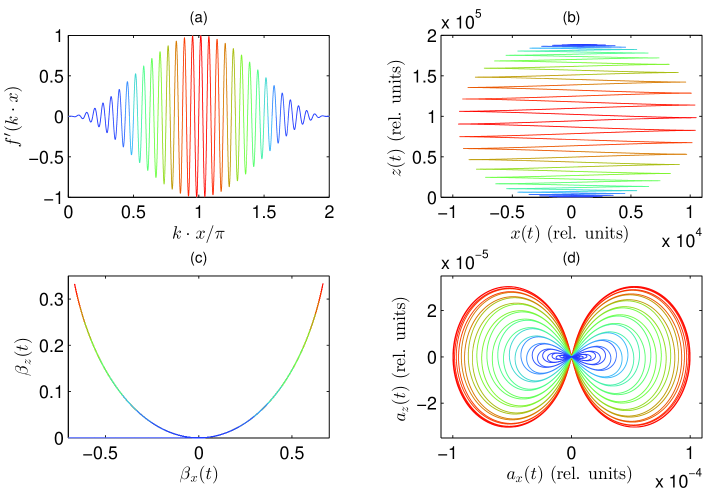
Figure 1: (Color online) In panel (a), the shape function $f^{\prime}(k\cdot x)$ defining the electric and magnetic field components of the 32-cycle laser pulse is shown for $T_{\mathrm{d}}=0$ and $N_{\mathrm{rep}}=1$. In the remaining panels, the solution of the relativistic Newton-Lorentz equation (1) for the electron moving in the depicted laser pulse is presented (i.e., electron position, speed, and acceleration). The parameters of the pulse are such that $\mu=1$, $\omega_{\rm L}=10^{-4}m_{\rm e}c^{2}$, and $N_{\rm osc}=32$, where the scaled amplitude of vector potential, $\mu$, measures the peak intensity of the laser field. Initially, the electron is at rest in the center of the coordinate system.

In our investigations we use the plane-wave-fronted pulse approximation. An applicability of this approximation is based on the assumption that the transverse variation of the electron trajectory in the laser field is negligible when compared to the size of the laser focus, as illustrated in Fig. 1. In Fig. 1(a), we present the solution of the relativistic Newton-Lorentz equation (1) for the electron initially at rest and in the presence of the laser pulse. The carrier frequency of the laser field $\omega_{\rm L}$ is equal to $10^{-4}m_{\rm e}c^{2}$ (which corresponds to the laser photon energy of about 50 eV), $N_{\rm osc}=32$, $N_{\rm rep}=1$, $T_{\mathrm{d}}=0$, and $\mu=1$. The conditions are set such that initially the electron is at rest in the center of the coordinate system, so its velocity is zero before the arrival of the laser pulse. Fig. 1(b) depicts the $x$- and $z$-coordinates of the electron’s position, Fig. 1(c) – the reduced velocity, and Fig. 1(d) – the acceleration of the electron. The colors of these distributions correspond to the colors of the laser pulse [Fig. 1(a)]. It turns out, that for higher amplitudes of the field depicted in Fig. 1(a), the trajectory of the electron preserves its shape form [Fig. 1(b)]; however, the values of the speed components $\beta_{x}(t)$ and $\beta_{z}(t)$ [Fig. 1(c)] attain higher values.

As one can see from Fig. 1, the classical electron placed in a linearly polarized laser field exhibits an oscillatory motion along the direction of the electric field component (i.e., along the $x$-axis) together with a drift motion in the propagation direction of the laser pulse (i.e., in the $z$-direction). It may also be observed that for a given laser field frequency the displacement of the electron is larger for a stronger laser field than for a weaker laser field. A useful measure of the relativistic length unit is the reduced electron Compton wavelength

$$\lambdabar_{\rm C}=\frac{\hbar}{m_{\rm e}c}=3.8616\times 10^{-13}\,{\rm m}\,,$$

which equals 1 in relativistic units. Note that for the chosen laser field parameters the electron displacement along the electric field vector is of the order of $10^{-9}$m (Fig. 1). Taking this into account, we find that the electron displacement along the electric field direction is of the order of $0.001\mu$m. For lasers available today, a typical linear dimension of their focus is a few $\mu$m. Therefore, the electron displacement in the transverse direction (even for very powerful laser fields) can be neglected on the scale of the focus, provided that the laser frequency is sufficiently large in the reference frame in which initially electrons are at rest. We conclude that the plane-wave-fronted pulse approximation is perfectly suitable for describing the nonlinear Thomson scattering processes generated by currently available laser sources.

III Nonlinear Compton scattering

Using the $S$-matrix formalism of strong-field QED, we derive that the probability amplitude for the Compton process, $e^{-}_{\bm{p}_{\mathrm{i}}\lambda_{\mathrm{i}}}\rightarrow e^{-}_{\bm{p}_{\mathrm{f}}\lambda_{\mathrm{f}}}+\gamma_{\bm{K}\sigma}$, with the initial and final electron momenta and spin polarizations $\bm{p}_{\mathrm{i}}\lambda_{\mathrm{i}}$ and $\bm{p}_{\mathrm{f}}\lambda_{\mathrm{f}}$, respectively, equals

$${\cal A}(e^{-}_{\bm{p}_{\mathrm{i}}\lambda_{\mathrm{i}}}\rightarrow e^{-}_{\bm{p}_{\mathrm{f}}\lambda_{\mathrm{f}}}+\gamma_{\bm{K}\sigma})=-\mathrm{i}e\int\mathrm{d}^{4}{x}\,j^{(++)}_{\bm{p}_{\mathrm{f}}\lambda_{\mathrm{f}},\bm{p}_{\mathrm{i}}\lambda_{\mathrm{i}}}(x)\cdot A^{(-)}_{\bm{K}\sigma}(x),$$ (14)

where $\bm{K}\sigma$ denotes the Compton photon momentum and polarization. Here, we consider the case when both the laser pulse and the Compton photon are linearly polarized. In Eq. (14),

$$A^{(-)}_{\bm{K}\sigma}(x)=\sqrt{\frac{1}{2\varepsilon_{0}\omega_{\bm{K}}V}}\,\varepsilon_{\bm{K}\sigma}\mathrm{e}^{\mathrm{i}K\cdot x},$$ (15)

where $V$ is the quantization volume, $\omega_{\bm{K}}=cK^{0}=c|\bm{K}|$ ($K\cdot K=0$), and $\varepsilon_{\bm{K}\sigma}=(0,\bm{\varepsilon}_{\bm{K}\sigma})$ are the polarization four-vectors satisfying the conditions

$$K\cdot\varepsilon_{\bm{K}\sigma}=0,\quad\varepsilon_{\bm{K}\sigma}\cdot\varepsilon_{\bm{K}\sigma^{\prime}}=-\delta_{\sigma\sigma^{\prime}},$$ (16)

for $\sigma,\sigma^{\prime}=1,2$. Moreover, $j^{(++)}_{\bm{p}_{\mathrm{f}}\lambda_{\mathrm{f}},\bm{p}_{\mathrm{i}}\lambda_{\mathrm{i}}}(x)$ is the matrix element of the electron current operator with its $\nu$-component equal to

$$[j^{(++)}_{\bm{p}_{\mathrm{f}}\lambda_{\mathrm{f}},\bm{p}_{\mathrm{i}}\lambda_{\mathrm{i}}}(x)]^{\nu}=\bar{\psi}^{(+)}_{\bm{p}_{\mathrm{f}}\lambda_{\mathrm{f}}}(x)\gamma^{\nu}\psi^{(+)}_{\bm{p}_{\mathrm{i}}\lambda_{\mathrm{i}}}(x).$$ (17)

Here, $\psi^{(+)}_{\bm{p}\lambda}(x)$ is the so-called Volkov solution of the Dirac equation coupled to the electromagnetic field Volkov ; KK (see, also Refs. Varro:A ; Varro:B ; Raicher2013 for possible generalizations)

$$\psi^{(+)}_{\bm{p}\lambda}(x)=\sqrt{\frac{m_{\mathrm{e}}c^{2}}{VE_{\bm{p}}}}\Bigl{(}1-\frac{e}{2k\cdot p}\not{A}\not{k}\Bigr{)}u^{(+)}_{\bm{p}\lambda}\mathrm{e}^{-\mathrm{i}S_{p}^{(+)}(x)},$$ (18)

with

$$S_{p}^{(+)}(x)=p\cdot x+\int^{k\cdot x}\Bigl{[}\frac{eA(\phi)\cdot p}{k\cdot p}-\frac{e^{2}A^{2}(\phi)}{2k\cdot p}\Bigr{]}{\rm d}\phi.$$ (19)

Moreover, $E_{\bm{p}}=cp^{0}$, $p=(p^{0},\bm{p})$, $p\cdot p=m_{\mathrm{e}}^{2}c^{2}$, and $u^{(+)}_{\bm{p}\lambda}$ is the free-electron bispinor normalized such that

$$\bar{u}^{(+)}_{\bm{p}\lambda}u^{(+)}_{\bm{p}\lambda^{\prime}}=\delta_{\lambda\lambda^{\prime}}.$$ (20)

The four-vector potential $A(k\cdot x)$ in Eq. (18) represents an external electromagnetic radiation generated by lasers, in the case when a transverse variation of the laser field in a focus is negligible. In other words, $A(k\cdot x)$ represents the plane-wave-fronted pulse. In this case, $k\cdot A(k\cdot x)=0$ and $k\cdot k=0$, which allows one to exactly solve the Dirac equation for such electromagnetic fields.

The probability amplitude for the Compton process (14) becomes

$${\cal A}(e^{-}_{\bm{p}_{\mathrm{i}}\lambda_{\mathrm{i}}}\longrightarrow e^{-}_{\bm{p}_{\mathrm{f}}\lambda_{\mathrm{f}}}+\gamma_{\bm{K}\sigma})=\mathrm{i}\sqrt{\frac{2\pi\alpha c(m_{\mathrm{e}}c^{2})^{2}}{E_{\bm{p}_{\mathrm{f}}}E_{\bm{p}_{\mathrm{i}}}\omega_{\bm{K}}V^{3}}}\,\mathcal{A},$$ (21)

where

$$\mathcal{A}=\int\mathrm{d}^{4}{x}\,\bar{u}^{(+)}_{\bm{p}_{\mathrm{f}}\lambda_{\mathrm{f}}}\Bigl{(}1-\mu\frac{m_{\mathrm{e}}c}{2p_{\mathrm{f}}\cdot k}f(k\cdot x)\not{\varepsilon}\not{k}\Bigr{)}\not{\varepsilon}_{\bm{K}\sigma}\,\Bigl{(}1+\mu\frac{m_{\mathrm{e}}c}{2p_{\mathrm{i}}\cdot k}f(k\cdot x)\not{\varepsilon}\not{k}\Bigr{)}u^{(+)}_{\bm{p}_{\mathrm{i}}\lambda_{\mathrm{i}}}\,\mathrm{e}^{-\mathrm{i}S(x)},$$ (22)

with

$$S(x)=S^{(+)}_{{p}_{\mathrm{i}}}(x)-S^{(+)}_{{p}_{\mathrm{f}}}(x)-K\cdot x\,.$$ (23)

While moving in a laser pulse, the electron acquires an additional momentum shift Compton ; BW , this leads to a notion of the laser-dressed momentum:

$$\bar{p}=p-\mu m_{\rm e}c\frac{p\cdot\varepsilon}{p\cdot k}\left\langle f\right\rangle k+\frac{1}{2}(\mu m_{\rm e}c)^{2}\frac{1}{p\cdot k}\left\langle f^{2}\right\rangle k\,.$$ (24)

Having this in mind we can define

$$N_{\rm eff}=\frac{K^{0}+\bar{p}^{0}_{\rm f}-\bar{p}^{0}_{\rm i}}{k^{0}}=cT_{\rm p}\frac{K^{0}+\bar{p}^{0}_{\rm f}-\bar{p}^{0}_{\rm i}}{2\pi},$$ (25)

which is both gauge- and relativistically invariant Compton .

The frequency-angular distribution of energy of the emitted photons for an unpolarized electron beam is given by

$$\frac{{\rm d^{3}}E_{\rm C}}{{\rm d}\omega_{\bm{K}}{\rm d^{2}}\Omega_{\bm{K}}}=\frac{1}{2}\sum_{\sigma=1,2}\sum_{\lambda_{\rm i}=\pm}\sum_{\lambda_{\rm f}=\pm}\frac{{\rm d^{3}}E_{{\rm C},\sigma}(\lambda_{\rm i},\lambda_{\rm f})}{{\rm d}\omega_{\bm{K}}{\rm d^{2}}\Omega_{\bm{K}}},$$ (26)

where

$$\frac{{\rm d^{3}}E_{{\rm C},\sigma}(\lambda_{\rm i},\lambda_{\rm f})}{{\rm d}\omega_{\bm{K}}{\rm d^{2}}\Omega_{\bm{K}}}=\alpha\left|\mathcal{A}_{{\rm C},\sigma}(\omega_{\bm{K}},\lambda_{\rm i},\lambda_{\rm f})\right|^{2},$$ (27)

and the scattering amplitude equals

$$\mathcal{A}_{{\rm C},\sigma}(\omega_{\bm{K}},\lambda_{\rm i},\lambda_{\rm f})=\frac{m_{\rm e}cK^{0}}{2\pi\sqrt{p_{\rm i}^{0}k^{0}(k\cdot p_{\rm f})}}\sum_{N}D_{N}\frac{1-{\rm e}^{-2\pi{\rm i}(N-N_{\rm eff})}}{{\rm i}(N-N_{\rm eff})},$$ (28)

with the functions $D_{N}$ defined in Compton .

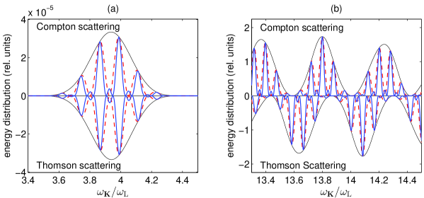
Figure 2: (Color online) The energy distribution of radiation emitted by the scattered electron. The black solid line corresponds to $N_{\text{rep}}=1$, the red dashed line to $N_{\text{rep}}=2$, whereas the blue solid line is for $N_{\text{rep}}=3$. Each subpulse contains eight field oscillations ($N_{\rm osc}=8$). The detection angles are $\varphi_{\bm{K}}=0$ and $\theta_{\bm{K}}=\pi/10$. While the results presented in panel (a) relate to $\mu=1$ and $\omega_{\text{L}}=3\times 10^{-3}m_{\text{e}}c^{2}$, the results presented in panel (b) are for $\mu=10$ and $\omega_{\text{L}}=3\times 10^{-2}m_{\text{e}}c^{2}$.

In Fig. 2, we compare the Thomson and Compton energy distributions for a single laser pulse in the reference frame in which initially electrons are at rest. As expected, for $\omega_{\bm{K}}\ll m_{\mathrm{e}}c^{2}$ both theories give the same results, as depicted in the left panel. However, for larger laser carrier frequency $\omega_{\mathrm{L}}$ and energies of generated photons $\omega_{\bm{K}}$ the Compton distribution is red-shifted with respect to the Thomson one. Such a shift has been analyzed in Seipt within the slowly changing envelope approximation. This analysis has been extended to arbitrarily short laser pulses in KrajewskaNewArchive2 , together with the discussion of the significant role played by the polarization of emitted radiation and the spin degrees of freedom of the electron initial and final states.

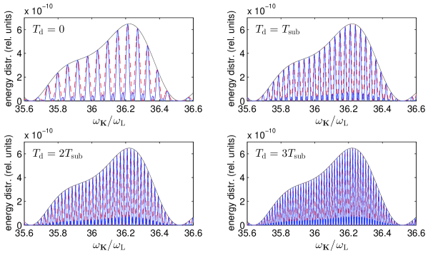
Figure 3: (Color online) The Compton energy distribution for the laser pulse parameters: $\omega_{\rm L}=4.15\times 10^{-4}m_{\rm e}c^{2}$, $\mu=1$, $N_{\rm osc}=16$, $\theta_{\bm{K}}=0.2\pi$, $\varphi_{\bm{K}}=0$, and $\chi=\pi$. Different panels correspond to four different delay times $T_{\mathrm{d}}$. The solid black lines (envelopes) present the energy distributions for a single pulse ($N_{\mathrm{rep}}=1$), the dashed red lines are for $N_{\mathrm{rep}}=2$, whereas the solid blue lines are for $N_{\mathrm{rep}}=3$. The corresponding energy distributions are divided by $N_{\mathrm{rep}}^{2}$, which proves the coherent properties of the generated high-order harmonics comb structures.

IV Compton high-order harmonics and generation of ultra-short pulses

High-order harmonics generated via non-relativistic interaction of intense laser pulses with atoms allow to synthesize attosecond pulses of coherent radiation Farkas . Currently, the energy bandwidth of the harmonic plateau can reach a few keV Popmintchev . In order to extend this spectrum up to MeV domain a relativistic treatment is necessary. The Compton process offers such a possibility, as it is presented in Fig. 3. For a single laser pulse ($N_{\rm rep}=1$), we observe a broad and smooth energy distribution from which we choose a part of the bandwidth approximately equal to the carrier frequency $\omega_{\mathrm{L}}$. However, if we apply the sequence of $N_{\mathrm{rep}}$ pulses the energy distribution shows an equally spaced peaks with maxima which scale as $N_{\mathrm{rep}}^{2}$. This scaling law indicates that the generated comb structure is temporarily coherent. Moreover, the distance between the peaks can be controlled by a delay of the laser subpulses. Therefore, one can interpret the emergence of such a structure as the result of the interference of Compton photons emitted from different subpulses KrajewskaNewArchive .

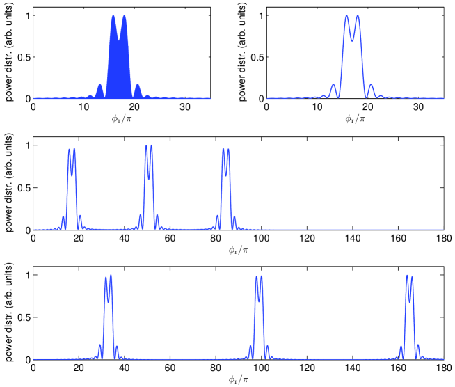
Figure 4: (Color online) Temporal power distributions of generated radiation, synthesized from the Compton amplitude (28) for $\lambda_{\mathrm{i}}\lambda_{\mathrm{f}}=1$ and for the laser field parameters specified in Fig. 3. The upper two panels show the power distributions defined by Eqs. (29) and (31) for a single pulse ($N_{\rm rep}=1$), after being normalized to the maximum value. The middle and the bottom panels show the temporal power distributions (31) composed from the energy distributions represented in Fig. 3 by the blue lines ($N_{\mathrm{rep}}=3$) for $T_{\mathrm{d}}=0$ and $T_{\mathrm{d}}=T_{\mathrm{sub}}$, respectively.

In order to further investigate the coherent properties of such a high-order harmonic spectrum let us consider the temporal power distribution of emitted radiation. This power distribution is related to the Compton amplitude (28) by the formula

$$\frac{\mathrm{d}^{2}P_{\mathrm{C},\sigma}(\phi_{\mathrm{r}},\lambda_{\rm i},\lambda_{\rm f})}{\mathrm{d}^{2}\Omega_{\bm{K}}}=\frac{\alpha}{\pi}\bigl{(}\Re\tilde{\mathcal{A}}^{(+)}_{\mathrm{C},\sigma}(\phi_{\mathrm{r}},\lambda_{\rm i},\lambda_{\rm f})\bigr{)}^{2}.$$ (29)

where

$$\tilde{\mathcal{A}}^{(+)}_{\mathrm{C},\sigma}(\phi_{\mathrm{r}},\lambda_{\rm i},\lambda_{\rm f})=\int_{0}^{\infty}\mathrm{d}\omega\mathcal{A}_{\mathrm{C},\sigma}(\omega,\lambda_{\rm i},\lambda_{\rm f})\mathrm{e}^{-\mathrm{i}\omega\phi_{\mathrm{r}}/\omega_{\mathrm{L}}}.$$ (30)

Here, $\Re$ denotes the real part and $\phi_{\mathrm{r}}=\omega_{\mathrm{L}}(t-R/c)$, with $R$ being a distance from the scattering region to the observation point. In general, the power distribution (29) is a very rapidly oscillating function of time. One can define the temporal power distribution of generated radiation, avaraged over these oscillations,

$$\frac{\mathrm{d}^{2}\langle P_{\mathrm{C},\sigma}\rangle(\phi_{\mathrm{r}},\lambda_{\rm i},\lambda_{\rm f})}{\mathrm{d}^{2}\Omega_{\bm{K}}}=\frac{\alpha}{2\pi}|\tilde{\mathcal{A}}^{(+)}_{\mathrm{C},\sigma}(\phi_{\mathrm{r}},\lambda_{\rm i},\lambda_{\rm f})|^{2}.$$ (31)

Fig. 4 depicts the temporal power distributions, (29) or (31), as functions of the dimensionless retarded phase $\phi_{\mathrm{r}}=\omega_{\mathrm{L}}(t-R/c)$, instead of the observation time $t$. The power distributions have been synthesized from the energy distributions presented in Fig. 3. As we see, the radiation is emitted in the form of short pulses. Similar conclusions can be drawn from the classical Thomson scattering, although some significant discrepancies between the classical and quantum theories can be observed KTK .

V Conclusions

In this paper, we have presented the theory of Thomson and Compton processes in intense laser pulses. We have shown that, by applying the sequence of laser pulses, it is possible to create high-order harmonics structures in the emitted radiation. We have investigated this problem in the electron beam reference frame. It appears, however, that in the laboratory frame, when electrons have the energy of the order of GeV, the bandwidth of the generated harmonic spectrum is of the order of a few MeV. This can be further synthesized into zepto- or even yoctosecond pulses, as will be presented elsewhere KTK .

References

- (1) Ehlotzky F, Krajewska K and Kamiński J Z 2009 Rep. Prog. Phys. 72 046401
- (2) Di Piazza A, Müller C, Hatsagortsyan K Z and Keitel C H 2012 Rev. Mod. Phys. 84 1177
- (3) Furry W H 1951 Phys. Rev. 81 115
- (4) Lau L L, He F, Umstadter D P and Kowalczyk R 2003 Phys. Plasmas 10 2155
- (5) Umstadter D P 2003 J. Phys. D 36 R151
- (6) Jackson J D 1998 Classical Electrodynamics (New York: John Wiley & Sons)
- (7) Landau L D and Lifshitz E M 1980 The Classical Theory of Fields (Portsmouth, NH: Heinemann)
- (8) Neville R A and Rohrlich F 1971 Phys. Rev. D 3 1692
- (9) Brown L S and Kibble T W B 1964 Phys. Rev. 133 A705
- (10) Goldman I 1964 Sov. Phys. JETP 46 1412
- (11) Nikishov A I and Ritus V I 1964 Sov. Phys. JETP 19 1191
- (12) Sengupta N D 1949 Bull. Math. Soc. 41 187
- (13) Vaschaspati 1962 Phys. Rev. 128 664
- (14) Vaschaspati 1963 Phys. Rev. 130 E2598
- (15) Sarachik E S and Schappert G T 1970 Phys. Rev. D 1 2738
- (16) Esarey E, Ride S K and Sprangle P 1993 Phys. Rev. E 48 3003
- (17) Ride S K, Esarey E and Baine M 1995 Phys. Rev. E 52 5425
- (18) Salamin Y I and Faisal F H M 1996 Phys. Rev. A 54 4383
- (19) Salamin Y I and Faisal F H M 1997 Phys. Rev. A 55 3964
- (20) Salamin Y I and Faisal F H M 1998 J. Phys. A 31 1319
- (21) Goreslavskii S P, Popruzhenko S V and Shcherbachev O V 1999 Laser Phys. 9 1039
- (22) Panek P, Kamiński J Z and Ehlotzky F 2002 Phys. Rev. A 65 022712
- (23) Ivanov D Y, Kotkin G L and Serbo V G 2004 Eur. Phys. J. C 36 127
- (24) Hartin A and Moortgat-Pick G 2011 Eur. Phys. J. C 71 1729
- (25) Popa A 2011 Phys. Rev. A 84 023824
- (26) Popa A 2012 Laser Part. Beams 30 591
- (27) Narozhny N B and Fofanov M S 1996 Sov. Phys. JETP 83 14
- (28) Voroshilo A I, Roshchupkin S P and Nedoreshta V N 2011 Laser Phys. 21 1675
- (29) Roshchupkin S P, Lebed’ A A, Padusenko E A and Voroshilo A I 2012 Laser Phys. 22 1113
- (30) Boca M and Florescu V 2009 Phys. Rev. A 80 053403
- (31) Mackenroth F, Di Piazza A and Keitel C H 2010 Phys. Rev. Lett. 105 063903
- (32) Seipt D and Kämpfer B 2011 Phys. Rev. A 83 022101
- (33) Mackenroth F and Di Piazza A 2011 Phys. Rev. A 83 032106
- (34) Boca M and Florescu V 2011 Eur. Phys. J. D 61 449
- (35) Krajewska K and Kamiński J Z 2012 Phys. Rev. A 85 062102
- (36) Boca M, Dinu V and Florescu V 2012 Phys. Rev. A 86 013414
- (37) Krajewska K and Kamiński J Z 2013 Laser Part. Beams 31 503
- (38) Bulanov S V et al. 2011 Nucl. Instrum. Methods Phys. Res. A 600 31
- (39) Leemans W P et al. 1996 Phys. Rev. Lett. 77 4182
- (40) Krajewska K and Kamiński J Z ArXiv:1307.5433
- (41) Griffiths D J 1999 Introduction to Electrodynamics (Englewood Cliffs, NJ: Prentice-Hall)
- (42) Volkov D M 1935 Z. Phys. 94 250
- (43) Krajewska K and Kamiński J Z 2010 Phys. Rev. A 82 013420
- (44) Varro S 2013 Laser Phys. Lett. 10 095301
- (45) Varro S ArXiv:1306:0097
- (46) Raicher E and Eliezer S 2013 Phys. Rev. A 88 022113
- (47) Krajewska K and Kamiński J Z 2012 Phys. Rev. A 86 052104
- (48) Krajewska K and Kamiński J Z ArXiv:1308.1663
- (49) Farkas G and Tóth C 1992 Phys. Lett. A 168 447
- (50) Popmintchev T et al. 2012 Science 336 1287
- (51) Krajewska K, Twardy M and Kamiński J Z ArXiv:1311.4872