Quantum Breathing Mode of Trapped Systems in One and Two Dimensions

Abstract

We investigate the quantum breathing mode (monopole oscillation) of trapped fermionic particles with Coulomb and dipole interaction in one and two dimensions. This collective oscillation has been shown to reveal detailed information on the many-particle state of interacting trapped systems and is thus a sensitive diagnostics for a variety of finite systems, including cold atomic and molecular gases in traps and optical lattics, electrons in metal clusters and in quantum confined semiconductor structures or nanoplasmas. An improved sum rule formalism allows us to accurately determine the breathing frequencies from the ground state of the system, avoiding complicated time-dependent simulations. In combination with the Hartree-Fock and the Thomas-Fermi approximations this enables us to extend the calculations to large particle numbers $N$ on the order of several million. Tracing the breathing frequency to large $N$ as a function of the coupling parameter of the system reveals a surprising difference of the asymptotic behavior of one-dimensional and two-dimensional harmonically trapped Coulomb systems.

Trapped systems are of major interest in many fields of research. Prominent examples are correlated electrons in metal clusters, e.g. [1], confined plasmas [2], ultracold quantum gases in traps or optical lattices [3, 4, 5], electrons in quantum dots [6, 7, 8, 9, 10] (“artificial atoms”), excitons in bilayers and quantum wells, e.g. [11, 12, 13, 14, 15] trapped ions [16], and colloidal particles [17]. Although these systems may differ in many physical details, their theoretical descriptions are often similar. A key property of finite systems in traps are the low-lying collective oscillations since they serve as a valuable diagnostic tool for the investigation of time-dependent and static features, e.g. [3, 18, 19]. The importance of these collective modes is comparable to that of spectroscopy in atomic systems. On the other hand, from the theoretical point of view, the calculation of normal modes is interesting as the results can be used to check the quality of models and of nonequilibrium simulations. In this work, we concentrate on the breathing mode – the (uniform) radial expansion and contraction of the system. This collective mode can easily be excited in experiments, e.g. by modulation of the confinement frequency or by a rapid compression or expansion [18].

For classical systems, the breathing mode is well understood [16, 20, 21]. However, if one incorporates quantum effects, the description of the mode becomes more complex. In our recent works [22, 23, 24], we reported results from time-dependent simulations and presented some unique properties of the quantum breathing mode. Among others, we discovered that the breathing mode comprises a superposition of at least two oscillations, which is a pure quantum effect. While one of the corresponding frequencies, $\omega_{\mathrm{cm}}$, has a universal value that equals twice the trap frequency, the other one, $\omega_{\mathrm{rel}}$, is strongly dependent on various system parameters. The goal of the present work is to determine how the frequency $\omega_{\mathrm{rel}}$ is influenced by, e. g., the particle number, the coupling parameter of the system, the dimension of the system and the type of binary interactions. These results are crucial for exploiting the above mentioned diagnostic potential of the breathing mode. An analysis for bosons with contact interaction in a one-dimensional trap that is complementary to ours is given in Ref. [25].

Most of the numerical results in our previous works are based on time-dependent approaches. The high numerical effort of these simulations poses strong restrictions on the accessibility of several physical parameters. In particular, the particle number usually does not exceed the values $N\approx 20$ in one-dimensional (1D) systems [24] and $N\approx 6$ in two-dimensional (2D) systems [26]. To overcome this problem, a simple semi-analytical estimator for the breathing frequency has been presented in our recent work [26]. As this estimator is solely based on equilibrium quantities, it enables one to save the computational effort of the time propagation in computer simulations, and, additionally, to use the breathing frequency as an experimental tool to determine the kinetic, trap and interaction energies of trapped systems. In [26], we validated the accuracy of the estimator, comparing its predictions with the results from correlated time-dependent calculations. In this work, we make use of it to describe physical situations for which no time-dependent calculations are available. We systematically study one- and two-dimensional systems of charged fermionic particles in the range from small finite systems to gases with many particles. Such a joint analysis of the dimensionality and the particle number has not been performed so far.

To work out how the equilibrium approach is connected to existing theories for the collective motions of many-body systems, we further extend the theoretical foundations of the breathing mode, providing a systematic description in terms of time-dependent perturbation theory. This allows one to conclude that the breathing mode is characterized by the spectrum of the initial Hamiltonian. To avoid an exact diagonalization of this Hamiltonian, we follow the well-known sum rule formalism [27, 28, 29, 30] to extract an approximation for the lowest excitation energy from the ground state. Furthermore, we show how to improve the sum rule formulas, which turns out to be important, especially for small systems. The sum rules allow us to apply ground-state methods with strongly reduced computational costs. Hence, we are able to considerably extend our previous results for fermionic particles with Coulomb interaction [24, 26]. The calculations are performed in the framework of the Hartree-Fock approximation, for small weakly coupled systems with significant finite-size effects, and the Thomas-Fermi approximation, for the transition to large systems. One of the major results from our analysis is that the dimension of the system has a strong influence on the qualitative behavior of large systems: With growing particle number, a one-dimensional system behaves more like an ideal quantum system (see also Ref. [24]), while a two-dimensional system, by contrast, approaches the classical limit. We show that this unexpected behavior is indicated by the lowest frequency of the breathing oscillation as well as a localization parameter which relates the average extension of the system to that of an ideal quantum system. Discussing how the total energies scale in non-interacting and strongly coupled (classical) systems, we further provide an explanation for the behavior in terms of simple quantities.

We start our presentation with a brief review of the quantum mechanical description of the trapped system. Expressing the excitation of collective modes in terms of time-dependent perturbation theory, we lay the foundation for the application of the sum rules. We briefly recapitulate the most important sum rule formulas and show how their accuracy can be improved. Using this formalism, we analyze how the breathing frequency depends on the particle number, the coupling parameter and the dimensionality of the system.

1 Theory

1.1 Time-dependent Schrödinger equation

We briefly recall the physical setting which has already been described in our previous works [22, 23, 24]. We aim at the quantum mechanical description of $N$ identical particles in a $d$-dimensional space. The time-evolution of the corresponding wave function is governed by the time-dependent Schrödinger equation (TDSE)

$$\mathrm{i}\frac{\mathrm{d}}{\mathrm{d}t}|\Psi(t)\rangle=\hat{H}(t)|\Psi(t)\rangle\;,$$ (1)

where we set $\hbar=1$. We assume that the Hamiltonian,

$$\hat{H}(t)=\hat{H}_{0}+\hat{H}_{1}(t)\;,$$ (2)

consists of the stationary part,

$$\hat{H}_{0}=\hat{T}+\hat{V}+\hat{W}\;,$$ (3)

and an additional perturbation term, $\hat{H}_{1}(t)$. The explicit form of $\hat{H}_{0}$ in the spatial coordinates $\mathbf{r}\equiv(\mathbf{r}_{1},\dots,\mathbf{r}_{N})$ is given by the kinetic energy

$$T(\mathbf{r})=\sum_{i=1}^{N}-\frac{1}{2m}\frac{\partial^{2}}{\partial\mathbf{r}_{i}^{2}}\;,$$ (4)

the trap energy

$$V(\mathbf{r})=\sum_{i=1}^{N}\frac{1}{2}m\Omega^{2}\mathbf{r}_{i}^{2}\;,$$ (5)

and the interaction energy

$$W(\mathbf{r})=\sum_{i<j}\frac{K_{\alpha}}{|\mathbf{r}_{i}-\mathbf{r}_{j}|^{\alpha}}\;.$$ (6)

If it is not further specified, we assume that the interaction is characterized by a repulsive power-law potential, $w(r)\propto 1/r^{\alpha}$, with the proportionality constant $K_{\alpha}$. Below we will concentrate on the important cases of Coulomb interaction ($\alpha=1$) and dipole interaction ($\alpha=3$). After rescaling all lengths, times and energies in terms of $l_{0}=\left(1/(m\Omega)\right)^{1/2}$, $\Omega^{-1}$ and $\Omega$, respectively, $\hat{H}_{0}$ takes the form

$${H}_{0}(\mathbf{r})=\frac{1}{2}\sum_{i=1}^{N}\left\{-\frac{\partial^{2}}{\partial\mathbf{r}_{i}^{2}}+\mathbf{r}_{i}^{2}\right\}+\sum_{i<j}\frac{\lambda}{|\mathbf{r}_{i}-\mathbf{r}_{j}|^{\alpha}}\;.$$ (7)

The dimensionless coupling parameter $\lambda>0$ determines the relative strength of the interaction energy [24]. It is given by

$$\lambda=\frac{1}{\hbar\Omega}\frac{K_{\alpha}}{l_{0}^{\alpha}}\;,$$ (8)

with, e. g., $K_{1}=q^{2}/(4\pi\epsilon)$, for the Coulomb interaction of particles with charge $q$ and the permittivity $\epsilon$, and $K_{3}=C_{\mathrm{dd}}/(4\pi)$ for the interaction of polarized magnetic or electric dipoles, with the corresponding proportionality constant $C_{\mathrm{dd}}$ [31]. While, in general, the interaction of two dipoles depends on their orientation, here we consider only the case of parallel dipoles [32, 33]. In experiments, parallel alignment perpendicular to the plane of the dipoles is typically realized with external fields.

1.2 Mode excitation

To formally include a weak mode excitation by an arbitrary operator $\hat{Q}$, acting only at the time $t=0$, we specify

$$\hat{H}_{1}(t)=\eta\delta(t)\hat{Q}\;,$$ (9)

where $\eta$ is a small real parameter. In the following, we assume that the eigenstates of $\hat{H}_{0}$ are given by $\left\{|0\rangle,|1\rangle,\dots\right\}$ with the corresponding eigenvalues $\left\{E_{0},E_{1},\dots\right\}$. Furthermore, the system is supposed to be initially in the ground state $|0\rangle$. With the help of first-order time-dependent perturbation theory, it can be shown that the time-dependent expectation value of an operator $\hat{A}$ without explicit time-dependence takes the form [24]

$$\langle\hat{A}\rangle(t)=\sum_{ij}c^{*}_{i}c_{j}\exp\left\{\mathrm{i}\left(E_{i}-E_{j}\right)t\right\}\langle i|\hat{A}|j\rangle$$ (10)

with the constant coefficients

$$c_{k}=\delta_{k,0}-\mathrm{i}\eta\langle k|\hat{Q}|0\rangle\;.$$ (11)

The breathing mode is excited by the monopole operator $\hat{Q}=\hat{\mathbf{r}}^{2}=\sum_{i}\hat{\mathbf{r}}_{i}^{2}$. For the typical observable $\hat{A}=\hat{\mathbf{r}}^{2}$, one can reduce Eq. (10) to the expression

$$\langle\hat{\mathbf{r}}^{2}\rangle(t)=\langle 0|\hat{\mathbf{r}}^{2}|0\rangle-{2\eta}\sum_{i}|\langle 0|\hat{\mathbf{r}}^{2}|i\rangle|^{2}\sin(\omega_{i,0}t)\;,$$ (12)

where $\omega_{i,0}=E_{i}-E_{0}$ are the mode frequencies. Equation (12) reveals that the quantum breathing mode is characterized by a superposition of sinusoids with different frequencies. For a full characterization of the breathing mode, one has to calculate the eigenvalues of $\hat{H}_{0}$ and the matrix elements $\langle 0|\hat{\mathbf{r}}^{2}|i\rangle$.

1.3 Separation ansatz

Although the breathing motion comprises a variety of possible frequencies, it was shown in recent works [22, 23, 24] that the breathing mode is dominated by just two frequencies. One of these has the universal value $2\,\Omega$. This value can be explained by a formal decoupling of the wave function into a center-of-mass (CM) and a relative part,

$$|\Psi(t)\rangle=|\Psi_{\mathrm{cm}}(t)\rangle\otimes|\Psi_{\mathrm{rel}}(t)\rangle\;.$$ (13)

Such a decoupling is induced by the splitting of the Hamiltonian [34],

$$\hat{H}(t)=\hat{H}_{\mathrm{cm}}(t)+\hat{H}_{\mathrm{rel}}(t)\;,$$ (14)

where the contributions read

$$\hat{H}_{\mathrm{cm}}(t) =\frac{N}{2}\hat{\mathbf{P}}^{2}+\frac{N}{2}\hat{\mathbf{R}}^{2}+\eta\delta(t)N\hat{\mathbf{R}}^{2}\;,$$ (15)

$$\hat{H}_{\mathrm{rel}}(t) =\sum_{i<j}\Big{\{}\frac{1}{2N}\hat{\mathbf{p}}_{ij}^{2}+\frac{1}{2N}\hat{\mathbf{r}}_{ij}^{2}+\hat{w}(|\hat{\mathbf{r}}_{ij}|)+\eta\delta(t)\frac{1}{N}\hat{\mathbf{r}}_{ij}^{2}\Big{\}}\;.$$ (16)

Here, we have introduced the CM and relative contributions, according to

$$\hat{\mathbf{O}} =\frac{1}{N}\sum_{i=1}^{N}\hat{\mathbf{o}}_{i}\;,$$ (17)

$$\hat{\mathbf{o}}_{ij} =\hat{\mathbf{o}}_{i}-\hat{\mathbf{o}}_{j}\;.$$ (18)

Since Eq. (15) describes a non-interacting $d$-dimensional oscillator problem for the observables $\hat{T}_{\mathrm{cm}}=N\,\hat{\mathbf{P}}^{2}/2$ and $\hat{V}_{\mathrm{cm}}=N\,\hat{\mathbf{R}}^{2}/2$, one can conclude that the quantities $\langle\hat{V}\rangle(t)$ and $\langle\hat{T}\rangle(t)$ always contain oscillations with the frequency $\omega_{\mathrm{cm}}=2\,\Omega$. The contributions from the relative system, however, are non-trivial. Depending on the coupling parameter $\lambda$, the dominating frequency obtains the values $\sqrt{3}\,\Omega\leq\omega_{\mathrm{rel}}\leq 2\,\Omega$, for Coulomb interaction, and $2\,\Omega\leq\omega_{\mathrm{rel}}\leq\sqrt{5}\,\Omega$, for dipole interaction [22, 23, 35]. This frequency corresponds to the first monopole excitation in the relative system.

2 Sum rules

As has been shown, the value of $\omega_{\mathrm{rel}}$ can be extracted from the spectrum of $\hat{H}_{0}$. For more than just a few particles, however, an exact computation of the spectrum is impossible. Nevertheless, if it is possible to calculate the ground state of the system, one can make use of the quantum mechanical sum rules to gain some insight into the spectral properties. In this section, we give a brief review of the sum rules. Comprehensive overviews of the theory were presented for the study of collective resonances in nuclear physics [27, 28, 29, 30]. While the application to quantum gases has been subject of many recent investigations [36, 19, 37, 38], we use the sum rules for the description of few-particle systems. We show how the conventional sum rule formulas can be modified to achieve very accurate results even for such small systems.

2.1 Calculation of weighted moments

The weighted moments are defined by

$$m_{k}=\sum_{i=1}^{\infty}(E_{i}-E_{0})^{k}\,|\langle 0|\hat{Q}|i\rangle|^{2}\;,$$ (19)

for any operator $\hat{Q}$ and any integer number $k\in\mathbb{Z}$. Containing the exact excitation energies, the moments can be used to define average excitation energies

$$E_{k,l}=\left(\frac{m_{k}}{m_{k-l}}\right)^{1/l}\;,$$ (20)

for positive integer numbers $l$. In the literature [27], one often finds the quantities $E_{k,2}$ and $E_{k,1}$. The average excitation energies fulfill the relation

$$\dots\geq E_{k+2,1}\geq E_{k+2,2}\geq E_{k+1,1}\geq E_{k+1,2}\geq\dots$$ (21)

and, especially, [29]

$$\lim_{k\to-\infty}E_{k,1}=\omega_{a,0}\;,$$ (22)

where the index $a$ corresponds to the lowest state excited by the operator $\hat{Q}$. Instead of directly evaluating the sum in Eq. (19), one can make use of the sum rules to simplify selected moments. In the following, we will concentrate on the calculation of the moments $m_{3}$, $m_{1}$ and $m_{-1}$ for the monopole operator $\hat{Q}=\hat{\mathbf{r}}^{2}$. For $m_{1}$ and $m_{3}$, one finds the sum rules

$$m_{1} =\frac{1}{2}\langle 0|[\hat{Q},[\hat{H}_{0},\hat{Q}]]|0\rangle$$ (23)

$$=2\ \langle 0|\hat{\mathbf{r}}^{2}|0\rangle\;.$$ (24)

and

$$m_{3} =\frac{1}{2}\langle 0|[[\hat{Q},\hat{H}_{0}],[\hat{H}_{0},[\hat{H}_{0},\hat{Q}]]]|0\rangle$$ (25)

$$={8\langle\hat{T}\rangle+8\langle\hat{V}\rangle+2\alpha^{2}\langle\hat{W}\rangle}\;.$$ (26)

The latter result can be obtained, reducing Eq. (25) to the evaluation of commutators with the types $[\hat{\mathbf{p}}_{i},\hat{\mathbf{r}}_{j}]$ and $[\hat{\mathbf{p}}_{i},1/|\hat{\mathbf{r}}_{j}-\hat{\mathbf{r}}_{k}|^{\alpha}]$ for all occurring indices $i$, $j$, $k$. The moment $m_{-1}$ can be calculated by

$$m_{-1}=-\frac{\partial}{\partial\gamma}\langle\hat{\mathbf{r}}^{2}\rangle_{\gamma=1}\;,$$ (27)

where the expectation value refers to the ground state of the Hamiltonian

$$\hat{H}_{0}(\gamma):=\hat{T}+\gamma\hat{V}+\hat{W}\;.$$ (28)

This becomes clear if one writes the derivative in Eq. (27) as

$$\frac{\partial}{\partial\gamma}\langle\hat{\mathbf{r}}^{2}\rangle_{\gamma=1}=\lim_{\epsilon\to 0}\frac{\langle\hat{\mathbf{r}}^{2}\rangle_{\gamma=1+\epsilon}-\langle\hat{\mathbf{r}}^{2}\rangle_{\gamma=1}}{\epsilon}$$ (29)

and evaluates $\langle\hat{\mathbf{r}}^{2}\rangle_{\gamma=1+\epsilon}$ with stationary perturbation theory [29]. Henceforth, we will use the notation $\mathrm{sr}(k,k-l):=E_{k,l}$. With the moments $m_{3}$ and $m_{1}$, one obtains the convenient sum rule formula

$$\mathrm{sr}(3,1) =\left\{\left(2+\alpha\right)+\left(2-\alpha\right)\frac{\langle\hat{T}\rangle}{\langle\hat{V}\rangle}\right\}^{1/2}$$ (30)

$$=\left\{\left(2+\alpha\right)+\left(2-\alpha\right)\left(1-\frac{\alpha\langle\hat{W}\rangle}{2\langle\hat{V}\rangle}\right)\right\}^{1/2}\;.$$

The two different representations of $\mathrm{sr}(3,1)$ in Eq. (30) are due to the virial theorem

$$2\langle\hat{T}\rangle-2\langle\hat{V}\rangle+\alpha\langle\hat{W}\rangle=0\;.$$ (31)

For the special case of Coulomb interaction ($\alpha=1$), Eq. (30) has already been used by Sinha [39]. A similar result for contact interaction was derived by Stringari [38]. Furthermore, we mention that Eq. (30) is a quantum generalization of the formula by Olivetti et al. for classical systems [21]. A revealing property of Eq. (30) is the fact that it allows one to interpret the behavior of the breathing frequency with the ratios of the contributions to the total energy. Especially the classical limit, with $\langle\hat{T}\rangle/\langle\hat{V}\rangle=0$, and the ideal quantum limit, with $\langle\hat{W}\rangle/\langle\hat{V}\rangle=0$, are included.

Another sum rule formula we will use in this paper is given by

$$\mathrm{sr}(1,-1)=\left\{-2\frac{\langle\mathbf{r}^{2}\rangle}{\left[\partial\langle\mathbf{r}^{2}\rangle/\partial\gamma\right]_{\gamma=1}}\right\}^{1/2}\;.$$ (32)

It has been presented as a rigorous upper bound of the breathing frequency by Menotti and Stringari [19].

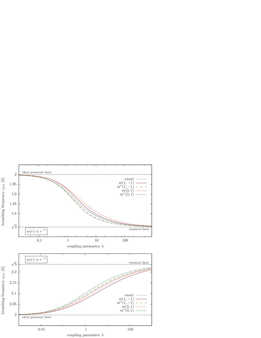
Figure 1: Comparison of the exact breathing frequencies, the conventional sum rule formulas and the improved sum rule formulas for a spin-polarized two-particle system in one dimension with Coulomb interaction (top) and dipole interaction (bottom).

2.2 Improved sum rule formulas

So far, we expressed the moments with the eigenstates and the eigenvalues of the full Hamiltonian $\hat{H}=\hat{H}_{\mathrm{rel}}+\hat{H}_{\mathrm{cm}}$. This may be disadvantageous for the estimation of $\omega_{\mathrm{rel}}$ if the weights of the center-of-mass terms are comparable to those of the relative terms. With the notations

$$\hat{\mathbf{R}}_{\mathrm{cm}}^{2}:=N\hat{\mathbf{R}}^{2}$$ (33)

and

$$\hat{\mathbf{r}}_{\mathrm{rel}}^{2}:=\frac{1}{N}\sum_{q<r}\hat{\mathbf{r}}^{2}_{qr}\;,$$ (34)

this can be understood more formally, expressing the moments as

$$m_{l} =\sum_{i=1}^{\infty}\left(E_{\mathrm{rel},i}-E_{\mathrm{rel},0}\right)^{l}|\langle 0_{\mathrm{rel}}|\hat{\mathbf{r}}_{\mathrm{rel}}^{2}|i_{\mathrm{rel}}\rangle|^{2}$$ (35)

$$\;\;\;+\sum_{k=1}^{\infty}\left(E_{\mathrm{cm},k}-E_{\mathrm{cm},0}\right)^{l}|\langle 0_{\mathrm{cm}}|\hat{\mathbf{R}}_{\mathrm{cm}}^{2}|k_{\mathrm{cm}}\rangle|^{2}\;.$$

Using the formulas $\mathrm{sr}(k,j)$, the contributions from the second sum in Eq. (35) may cause considerable inaccuracies of the estimator for $\omega_{\mathrm{rel}}=E_{\mathrm{rel},1}-E_{\mathrm{rel},0}$. Furthermore, it cannot be guaranteed that the sum rule formulas are upper bounds of the frequency $\omega_{\mathrm{rel}}$ if there exist non-vanishing contributions $E_{\mathrm{cm},k}-E_{\mathrm{cm},0}<\omega_{\mathrm{rel}}$. For example, this is the case for dipole interaction, where $\omega_{\mathrm{cm}}\leq\omega_{\mathrm{rel}}$ is valid for all coupling parameters. A simple solution to this problem is to eliminate the second sum in Eq. (35). As all terms are known analytically, this can simply be accomplished by introducing the corrected moments

$$m^{*}_{k}:=m_{k}-2^{k-1}d\;.$$ (36)

Using these moments, we introduce the following improved sum rule formulas,

$$\mathrm{sr}^{*}(k,k-l):=\left(\frac{m^{*}_{k}}{m^{*}_{k-l}}\right)^{1/l}\;.$$ (37)

These formulas are not only expected to yield more accurate results than the conventional formulas, they also restore the character of the approximation as an upper bound for all $\alpha$. The special case $\mathrm{sr}^{*}(3,1)$ is equivalent to the equilibrium formula presented in Ref. [26].

To demonstrate the difference between the formulas $\mathrm{sr}$ and $\mathrm{sr}^{*}$, we exactly determine the spectrum of the two-particle system. Expressing the relative vector $\mathbf{r}_{1,2}$ in the hyperspherical coordinates $\left(\rho,\phi_{1},\ldots,\phi_{d-1}\right)$ [40], one can reduce the relative problem to the equation

$$\bigg{\{}-\frac{1}{2}\frac{\mathrm{d^{2}}}{\mathrm{d}\rho^{2}}+\frac{\rho^{2}}{2}+\frac{\left(l+(d-2)/2\right)^{2}-1/4}{2\rho^{2}}+\frac{\lambda}{2^{\alpha/2}\rho^{\alpha}}-E_{\mathrm{rel}}\bigg{\}}u_{l}(\rho)=0\;.$$ (38)

We obtain the spectrum by solving the corresponding eigenvalue problem in the matrix representation that arises from the expansion of $u_{l}$ in terms of FEDVR basis functions (see Sec. 3.1). As the spectrum of the Hamiltonian $\hat{H}_{\mathrm{cm}}$ is known analytically, we can directly reconstruct the moments. In Fig. 1, we compare the exact breathing frequencies with the sum rule estimators for Coulomb and dipole interaction. In both cases, the improvement of the sum rules leads to a higher accuracy. For dipole interaction, it is shown that, in fact, the frequencies from the estimators $\mathrm{sr}(3,1)$ and $\mathrm{sr}(1,-1)$ are below the exact values. At the same time, it can be seen that this problem is solved by the improved formulas.

To conclude, we remark that the subtractive correction of the moments in Eq. (36) does not depend on the particle number. Therefore, it can be expected that the improvement of the sum rules is only important for small systems, where the eigenvalues of $\hat{H}_{\mathrm{rel}}$ and $\hat{H}_{\mathrm{cm}}$ are of the same order. Nevertheless, we stress the difference between the results, because the influence of the CM subsystem was not mentioned in some other works, e. g., Ref. [37] for the case of dipole interaction.

3 Numerical methods

In order to obtain the breathing frequencies of one- and two-dimensional systems, we calculate the ground-state energies and apply the sum rule formulas. We use the Hartree-Fock (HF) and the Thomas-Fermi (TF) approximation to cover the range from small to large systems. For comparison, we also show some exact configuration interaction (CI) and time-dependent Hartree-Fock (TDHF) results, which were obtained in our previous work [24]. In the following, some details of the methods are mentioned.

3.1 Hartree-Fock approximation

The Hartree-Fock approximation [41, 42] reduces the $N$-body problem to an effective one-body problem, where the interactions are taken into account on the mean-field level. The central idea of the HF method is to assume that the solution of the Schrödinger equation is a single Slater determinant

$$|\Psi\rangle=|\phi_{1}\dots\phi_{N}\rangle\;.$$ (39)

Requiring that the set of single-particle spin orbitals $|\phi_{1}\rangle,\dots|\phi_{N}\rangle$ minimizes the total energy $E=\langle\Psi|\hat{H}_{0}|\Psi\rangle$, one can derive the Hartree-Fock equations

$$\hat{F}|\phi_{k}\rangle=\epsilon|\phi_{k}\rangle\;,$$ (40)

where

$$\hat{F}=\hat{h}+\sum_{i=1}^{N}\hat{J}_{i}-\hat{K}_{i}$$ (41)

is the Fock operator. For the trapped system, $\hat{h}$ takes the form

$$h(\mathbf{r})=-\frac{1}{2}\frac{\partial^{2}}{\partial\mathbf{r}^{2}}+\frac{1}{2}\mathbf{r}^{2}\;.$$ (42)

The interaction is incorporated by the operators $\hat{J}_{i}$ and $\hat{K}_{i}$, which are defined by their actions

$$\hat{J}_{i}|\phi_{k}\rangle =\lambda\langle\phi_{i}|\hat{w}|\phi_{i}\rangle|\phi_{k}\rangle\;,$$ (43)

$$\hat{K}_{i}|\phi_{k}\rangle =\lambda\langle\phi_{i}|\hat{w}|\phi_{k}\rangle|\phi_{i}\rangle\;.$$ (44)

Expanding the spin orbitals in terms of a single-particle basis, we transfer the HF equations to a matrix equation. For one-dimensional systems, the utilized basis is a finite-element discrete variable representation [43, 44] (FEDVR). To avoid divergences, the Coulomb potential is regularized, according to the standard formula [22, 23]

$$w(|r-r^{\prime}|)=\frac{1}{\left[(r-r^{\prime})^{2}+\kappa^{2}\right]^{1/2}}\;.$$ (45)

with the screening parameter $\kappa$. In our recent work [24], we checked that converged results are obtained with $\kappa=0.1$. In two-dimensional systems, by contrast, such a screening is not necessary, as the basis is formed by the eigenfunctions of the harmonic oscillator in spherical coordinates. Our implementation for the calculation of the matrix elements is based on the code OpenFCI by Kvaal [45].

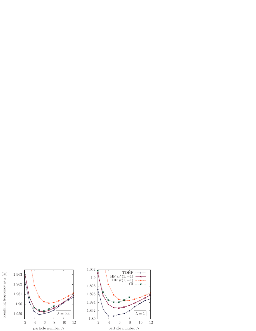
Figure 2: Breathing frequencies vs. particle number for a one-dimensional spin-polarized system with Coulomb interaction and different coupling parameters. The results from the improved sum rule formula yield more accurate results than the TDHF results from our previous work [24]. The missing points of the curves $\mathrm{sr}(1,-1)$ for $N=2$ have the values $1.972\,\Omega$ ($\lambda=0.3$) and $1.920\,\Omega$ ($\lambda=1$).

3.2 Thomas-Fermi approximation

For the extension of the HF results, we use the well-known Thomas-Fermi approximation [46, 47, 48, 49]. It is expected to yield the correct trend for large particle numbers, because the oscillations of the single-particle density – which are not shown by the density in TF approximation – become negligible [24].

In the one-dimensional case, the TF equation for spin-polarized particles reads

$$\frac{\pi^{2}}{2}n(r)^{2}+\frac{1}{2}r^{2}+\lambda\int\frac{n(r^{\prime})}{\left[(r-r^{\prime})^{2}+\kappa^{2}\right]^{1/2}}\mathrm{d}r^{\prime}=\mu\;,$$ (46)

where $\mu$ is the chemical potential. Fixing the particle number $N$ and requiring the normalization

$$\int n(r)\mathrm{d}r=N\;,$$ (47)

one has to find the density $n(r)$ and the corresponding chemical potential which solve Eq. (46). We obtained our results on a grid, according to the following scheme: For each considered particle number, we start our calculation with a very small coupling parameter $\lambda$. At this, we choose the initial trial density

$$n(r)=\frac{1}{\pi}\sqrt{2N-r^{2}}\;,$$ (48)

which is exact for a non-interacting system [50]. Updating the chemical potential and the density in a self-consistent procedure [51], we finally obtain the density that solves Eq. (46). After that, we slightly increase $\lambda$ and start a new calculation, where the initial density is the final density from the previous calculation. This procedure is repeated until some final value of $\lambda$ is reached.

For two-dimensional systems, we follow a simpler approach by Sinha [39]. Making the ansatz

$$n(\mathbf{r})=n(r)=\frac{1}{2\pi\gamma}(r_{0}^{2}-r^{2})$$ (49)

for the density, we determine the variational parameter $\gamma$ that minimizes the total energy

$$E=\frac{1}{3}N^{3/2}\frac{1}{\gamma^{1/2}}+\frac{1}{3}N^{3/2}\gamma^{1/2}+\lambda\frac{512}{315}\frac{\sqrt{2}}{\pi\gamma^{1/4}}N^{7/4}\;.$$ (50)

In this equation, the single terms correspond to the kinetic energy, the trap energy and the interaction energy in this order.

The method for the 2D case has the advantage that the parabolic ansatz for the density allows us to express the interaction energy analytically. In the 1D case, however, the calculations are more complex, because the integral

$$\lambda\int\frac{n(r^{\prime})}{\left[(r-r^{\prime})^{2}+\kappa^{2}\right]^{1/2}}\mathrm{d}r^{\prime}$$ (51)

has to be calculated for each grid point $r$ in each iteration step.

4 Results

We report the breathing frequencies for one- and two-dimensional systems. While only spin-polarized systems are treated in the 1D case, the occupation of the spin orbitals follows Hund’s rules in 2D systems. In the following, we consider the finite-size effects of small systems and the transition to large systems separately. In the end of this section, we explain the calculated breathing frequencies by the characteristics of the ground states.

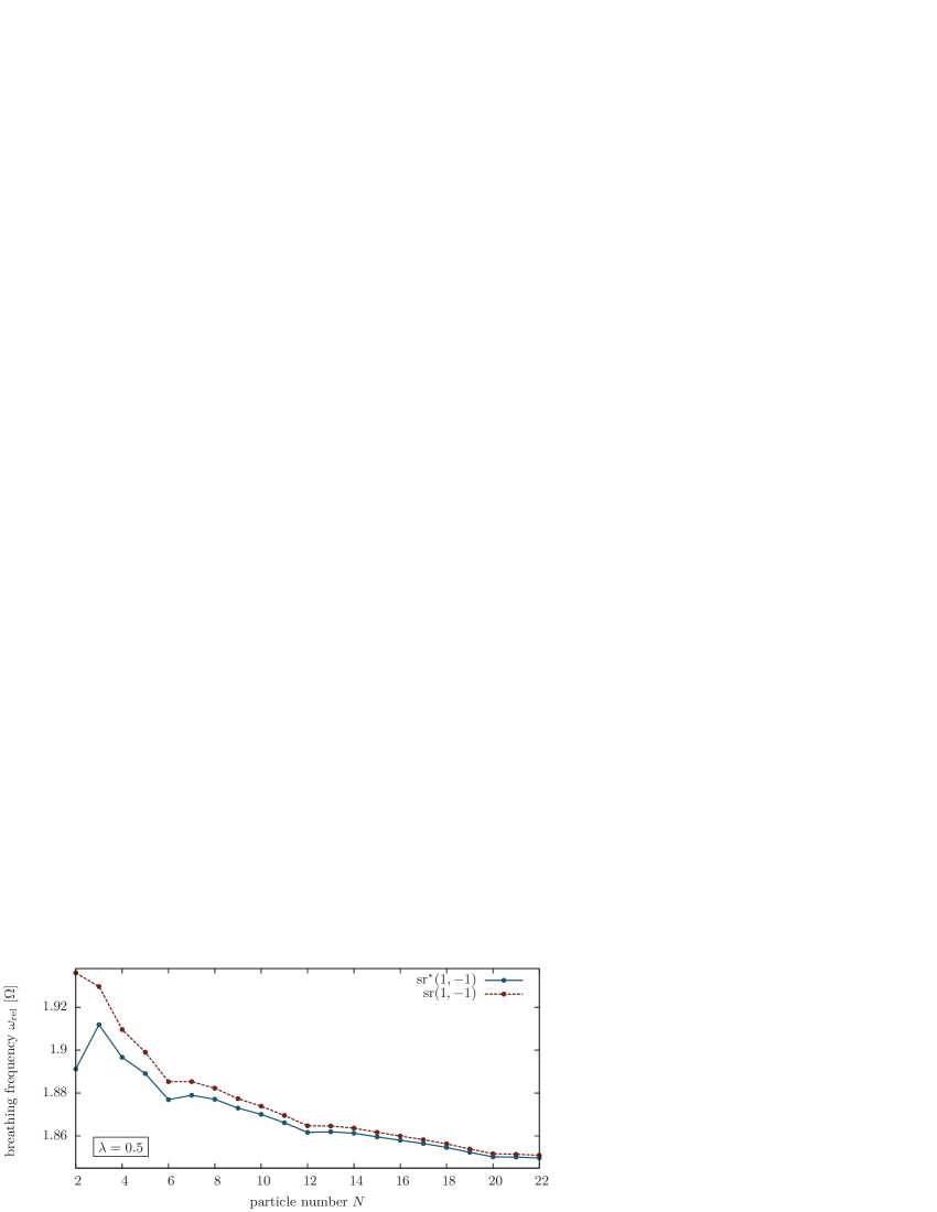
Figure 3: $N$-dependent breathing frequencies for Coulomb-interacting particles in two dimensions. The minima correspond to closed energy shells. For 2 and 3 particles, the improvement of the sum rule formulas is crucial for the correct qualitative description.

4.1 Small systems

4.1.1 1D

 
We start with an analysis of small one-dimensional systems. In Fig. 2, we compare the breathing frequencies from different methods for the coupling parameters $\lambda=0.3$ and $\lambda=1$. On the one hand, we show the time-dependent HF and CI results from our previous work [24]. On the other hand, we show the results obtained with static HF calculations in combination with the conventional and the improved sum rule formulas, respectively. One can draw the following conclusions: Comparing with the exact CI results, the results from the improved sum rule formulas are more accurate than the TDHF results. The improved accuracy of the sum rules can be explained by the fact that the static HF calculations could be performed with a larger basis than the time-dependent HF calculations. Furthermore, the error induced by the sum rules appears to be less important than the error induced by the HF approximation. Finally, one notices that the improvement of the sum rule formulas does not only lead to a higher accuracy for small particles, it also enables one to find the frequency minimum – which was already discovered in our previous work [24] – at the correct position $N=6$, instead of $N=7$. However, the figure already reveals that the difference between both formulas tends to vanish for large particle numbers.

4.1.2 2D

 
The step from 1D to 2D systems is usually numerically demanding, because – roughly estimated – the number of single-particle basis functions has to be squared. This is especially challenging for time-dependent calculations. However, using the sum rules and the HF method, we are able to investigate the finite-size effects of the breathing mode in 2D Coulomb systems for the first time. In Fig. 3, we show the frequencies for small ($N\leq 22$) systems with an intermediate coupling parameter $\lambda=0.5$. Compared to the one-dimensional systems, we observe that the non-monotonic behavior of the frequency has increased. More precisely, the frequency has local minima for 2, 6, 12 and 20 particles. These “magic” particle numbers are well-known from various experimental and theoretical studies of quantum dots [52, 53, 8]. The corresponding configurations are very stable, because they are characterized by closed energy shells. Typically, experimental evidence for the occurrence of the magic configurations is given by the measurement of $N$-dependent addition energies. Apparently, the breathing mode provides an alternative tool for the diagnostics of these properties. Furthermore, it has been shown recently that important system properties, such as the kinetic and potential energy, can be obtained from the results of the breathing frequency [26].

Using the HF approximation, we observe the same non-monotonic behavior for all coupling parameters $\lambda\leq 1$. Another important result is that – especially for 2 and 3 particles – the improvement of the sum rules is crucial to reproduce the correct behavior.

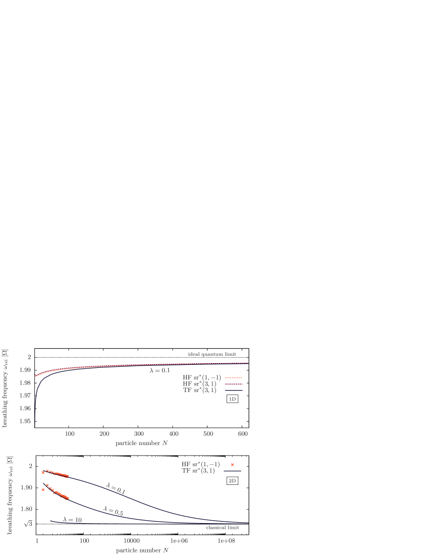
Figure 4: Behavior of the breathing frequencies for large particle numbers in 1D (top) and 2D (bottom).

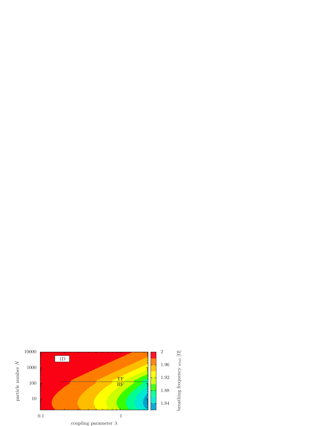
Figure 5: Breathing frequency of a Coulomb system in a one-dimensional harmonic trap in the $(\lambda,N)$-plane. The data were produced with the Thomas-Fermi approximation ($\mathrm{sr}^{*}(3,1)$, $N>100$) and the Hartree-Fock approximation ($\mathrm{sr}^{*}(1,-1)$, $N\leq 100$). The step around $N=100$ particles is due to the different approximation methods.

4.2 Large systems

4.2.1 1D

 
In our recent work [24], we found several hints that an increase of the particle number in one-dimensional systems leads to a steady increase of quantum effects. This means that the breathing frequency slowly transitions to the quantum limit $\omega_{\mathrm{rel}}=2\,\Omega$. However, the calculations of the frequencies were restricted to 20 particles with coupling parameters $\lambda\leq 1$. In this work, we extend the results, reporting the frequencies for up to 10000 particles with $\lambda\lesssim 2$.

To start the analysis for large systems, we compare the results from 1D HF calculations and the corresponding TF calculations for several hundred particles in the top plot of Fig. 4. As one can see, the difference between both approximations tends to vanish for large $N$. Hence, both approximations confirm the trend $\omega_{\mathrm{rel}}\to 2\,\Omega$ in the limit $N\to\infty$. For an overview, the contour plot in Fig. 5 summarizes the behavior of the breathing frequency in the $(\lambda,N)$-plane. For all coupling parameters, the contours have a small step around $N=100$, where the results from HF and TF calculations have been joined. Nevertheless, the plot is suitable to trace the finite size effects, with the frequency minima for $N=6$, as well as monotonic behavior of large systems.

As the frequencies approach the ideal limit only very slowly, we conclude with a remark that one can give a numerical proof for the large-$N$ behavior in the TF approximation. For that purpose, one uses the ideal density to calculate the kinetic energy, the trap energy and the interaction energy (with arbitrary fixed $\lambda$) as a function of the particle number. Such a calculation reveals that, for each coupling parameter $\lambda$, there exists a large particle number for which the interaction energy becomes negligible compared to the other two contributions. Consequently, the ideal density becomes a correct solution of Eq. (46) in the limit $N\to\infty$. In practice, that implies that an increase of $N$ leads to a faster convergence of the density if the initial guess in the self-consistent procedure is the ideal density.

4.2.2 2D

 
In two-dimensional systems, the $N$-dependent behavior of the breathing frequency is contrary to that of one-dimensional systems. In the bottom plot of Fig. 4, one can see that the frequency always reaches the value $\sqrt{3}\,\Omega$, in the limit $N\to\infty$. This behavior is confirmed for a broad range of coupling parameters in Fig. 6. Hence, 2D systems always approach the classical limit if either the particle number or the coupling parameter is increased.

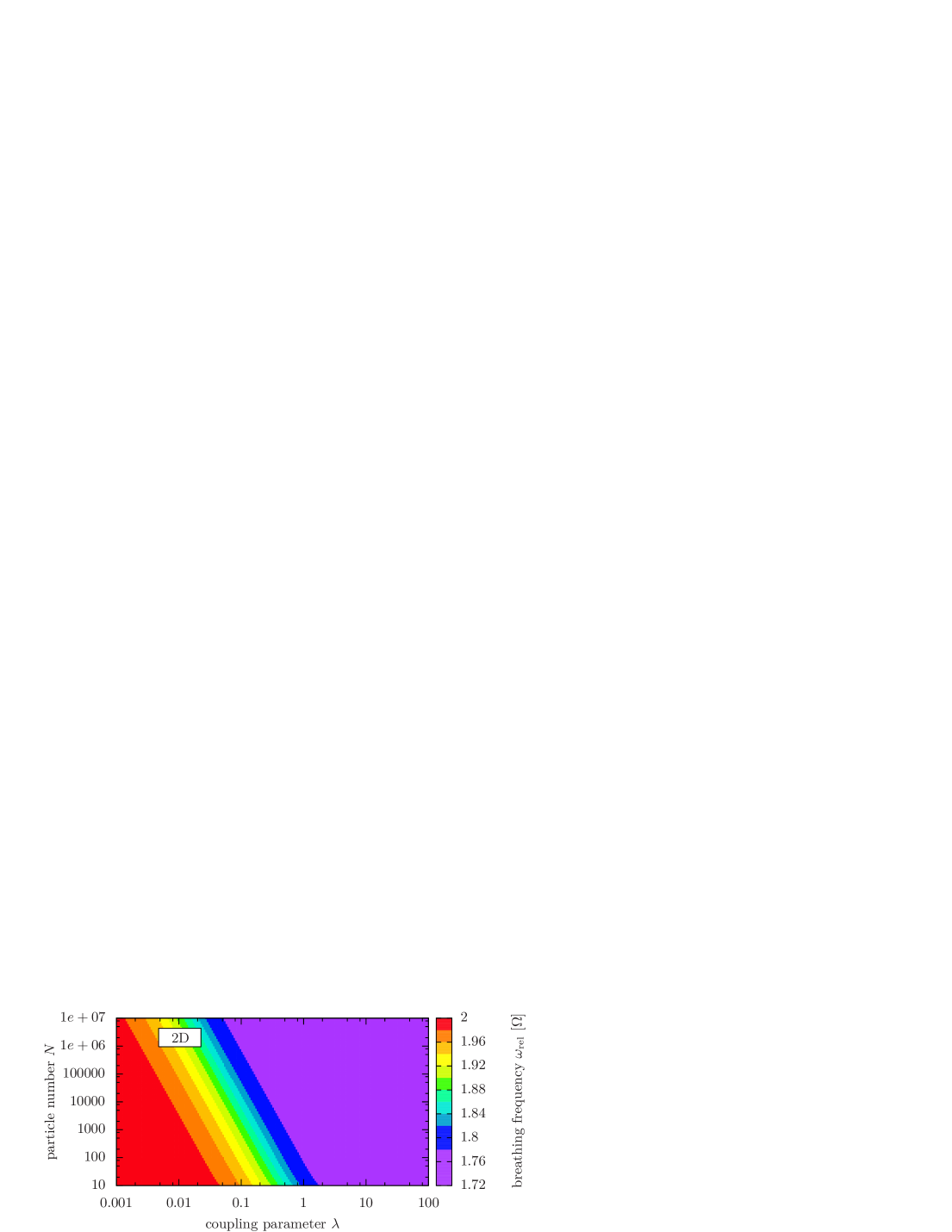
Figure 6: Breathing frequency of a Coulomb system in a two-dimensional harmonic trap in the $(\lambda,N)$-plane. The data were produced with the Thomas-Fermi approximation ($\mathrm{sr}^{*}(3,1)$).

Compared to the results for the 1D systems, the ranges of numerically accessable $\lambda$ and $N$ are much broader for 2D systems. This can be explained by the fact that the parabolic ansatz for the density profile in the Thomas-Fermi approximation, Eq. (49), is a drastic simplification of the problem. Hence, we can treat all coupling parameters with the same computational effort of a simple minimization procedure. Despite the restrictiveness of the parabolic ansatz, we can show that the results are fairly accurate. On the one hand, the good agreement of the TF and the HF results shown in Fig. 4 justifies the parabolic ansatz, at least for weakly coupled systems. On the other hand, to check that the ansatz can also be used to reproduce the correct energies of strongly coupled systems, we show the total energies for a broad range of coupling parameters and different particle numbers in Fig. 7. It turns out that – for sufficiently large particle numbers – the TF results converge to the results from classical molecular dynamics (MD) simulations in the limit of large $\lambda$.

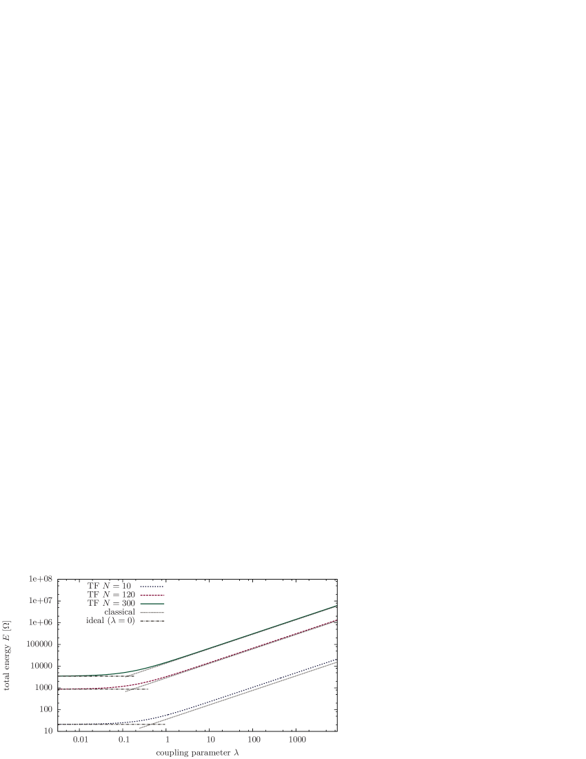
Figure 7: $\lambda$-dependent total energies of a 2D Coulomb system for different particle numbers. The results from the Thomas-Fermi approximation are compared to the results from classical molecular dynamics simulations and the analytical values of an ideal Fermi gas. An analogous figure with exact results for the 1D case is to be found in the work of Astrakharchik and Girardeau [50].

4.3 Explanation of the asymptotic behavior with ground-state properties

In the following, we provide some supportive explanation for the different behaviors of one- and two-dimensional systems. First, we trace the characteristics with the help of a localization parameter that measures the extension of the system. Second, we introduce a simple estimator for the distinction between quantum and classical systems.

4.3.1 Localization parameter

 
Being inspired by the degeneracy parameter of a macroscopic homogeneous electron gas, one can define a localization parameter for the trap. This parameter is meant to express the nonideality of the system with geometric quantities. An estimator for the mean extension of the system is given by

$$\sigma =\left\{2\langle\hat{V}\rangle\right\}^{1/2}\;.$$ (52)

For the non-interaction systems, it has the value

$$\sigma_{\mathrm{ideal}} =\frac{1}{\sqrt{2}}N\;, \qquad\mathrm{(1D)}\;,$$ (53)

$$\sigma_{\mathrm{ideal}} =\sqrt{2/3}N^{3/4}\;, \qquad\mathrm{(2D)}\;.$$ (54)

With this, one can define the localization parameter

$$\chi=\frac{\sigma_{\mathrm{ideal}}}{\sigma}\;,$$ (55)

which measures how much the extension of the system deviates from that of an ideal non-interacting quantum system. Starting with the value $\chi=1$ in the ideal system, the localization parameter decreases to zero in the course of the transition to the strongly coupled regime. In Fig. 8, we compare the localization parameter with the breathing frequency for one- and two-dimensional systems in the $(\lambda,N)$-plane. The data were produced with the Thomas-Fermi approximation and the frequencies were estimated with the sum rule formula $\mathrm{sr}^{*}(3,1)$. We concentrate on particle numbers $N\geq 100$ to make sure that finite-size effects are reduced. Furthermore, since the 1D TF method is reliable for small coupling parameters, we restrict the illustration to the regime $\lambda\lesssim 1$.

The figure shows that the localization parameter is well-suited to track the qualitative behavior of the breathing frequency. Equal values of $\chi$ correspond to equal values of the breathing frequency. To illustrate this, the plot shows exemplary dotted lines which indicate equal values of each quantity. In the logarithmic plot, these are straight lines. Remarkably, the lines for 1D systems have a positive slope, while the lines for 2D systems have a negative slope. The corresponding best fits in the ranges $100\leq N\leq 10000$ and $0.1\leq\lambda\leq 1$ read

$$N =(1.3\times 10^{4})\lambda^{2.45}\;, \qquad\mathrm{(1D)}\;,$$ (56)

$$N =100\lambda^{-4}\;, \qquad\mathrm{(2D)}\;.$$ (57)

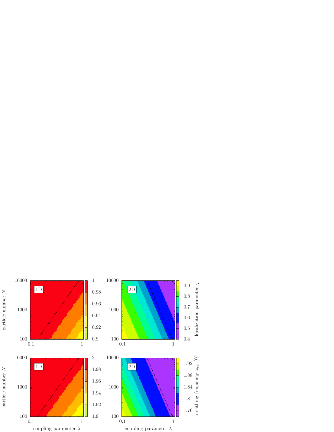
Figure 8: Comparison of the breathing frequencies (bottom) and the localization parameters (top) in the ($\lambda$,$N$)-plane for a 1D (left) and a 2D (right) trap. The dotted lines represent exemplary constant values.

4.3.2 Estimator for intermediate couplings

 
Finally, we provide another rough estimator for a supportive understanding of the observed behavior. For the two-dimensional system, the straight lines in Fig. 7 demonstrate that the total energies can be approximated by those from non-interacting Fermi gases for weak couplings,

$$E_{\mathrm{ideal}}^{\mathrm{2D}}=\frac{2}{3}N^{3/2}\;,$$ (58)

and those from purely classical systems for strong couplings,

$$E_{\mathrm{classical}}^{\mathrm{2D}}=K\lambda^{2/3}N^{5/3}\;.$$ (59)

The last equation is derived by setting the kinetic energy to zero and minimizing the remaining terms in Eq. (50). The constant $K$ has the value

$$K=\left(\frac{256\sqrt{2}}{315\pi}\right)^{2/3}+\frac{512\sqrt{2}}{315\pi}\left(\frac{256\sqrt{2}}{105\pi}\right)^{-1/3}\;.$$ (60)

As has been shown by Astrakharchik and Girardeau [50], one can also derive the corresponding terms for one-dimensional systems, where one obtains

$$E_{\mathrm{ideal}}^{\mathrm{1D}}=\frac{1}{2}N^{2}$$ (61)

for non-interacting systems and

$$E_{\mathrm{classical}}^{\mathrm{1D}}=\frac{3}{10}(3\lambda N\ln N)^{2/3}N$$ (62)

for classical systems. In both 1D and 2D, we use the quantities $E_{\mathrm{ideal}}$ and $E_{\mathrm{classical}}$ to define a regime of intermediate coupling. Taking account of the $\lambda$-dependence of the total energy shown in Fig. 7, we mark this region by the coupling parameter $\tilde{\lambda}$ for which the classical estimator $E_{\mathrm{classical}}$ is equal to the ideal estimator $E_{\mathrm{ideal}}$. One obtains

$$\tilde{\lambda}=\left(\frac{2}{3K}\right)^{3/2}N^{-1/4}$$ (63)

for 2D systems, which is in agreement with the functional form of Eq. (57). For the 1D systems, one obtains

$$\tilde{\lambda}=\frac{1}{3}\left(\frac{5}{3}\right)^{3/2}\frac{N^{1/2}}{\ln N}\;.$$ (64)

In this equation, the relation between $N$ and $\tilde{\lambda}$ slightly differs from that in Eq. (56). However, we expect that both definitions come to agreement if one covers a larger area of the ($\lambda,N$)-plane shown in Fig. 8.

The coupling parameter $\tilde{\lambda}$ roughly divides the systems into the ones with dominating quantum-like behavior ($\lambda<\tilde{\lambda}$) and the other ones with dominating classical behavior ($\lambda>\tilde{\lambda}$). Apparently, the trend for large systems is as follows: An increase of $N$ leads to a growing classical regime in 2D and a growing quantum regime in 1D. In Fig. 9, Eqs. (63) and (64) are plotted. Remarkably, for one-dimensional systems, $\tilde{\lambda}$ has a minimum for $N=7$ and thus even reproduces the non-monotonic behavior.

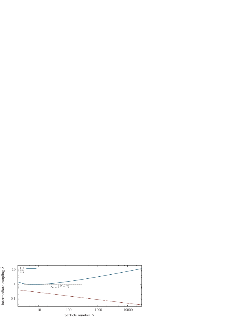
Figure 9: $N$-dependent behavior of the intermediate coupling parameter $\tilde{\lambda}$, for one- and two-dimensional systems.

5 Discussion

In this work, we presented an improvement of the conventional sum rule formulas for the calculation of the monopole excitation spectrum. The main idea was the elimination of the analytically known center-of-mass contributions to the weighted moments. It turned out that the improvement yields very accurate results for the frequencies of the quantum breathing mode.

In our previous work, we discussed that the breathing mode is an indicator for the nonideality of the system [24]. With Eq. (30), we can express this statement more precisely, mapping the breathing frequency to a fixed relation between the kinetic energy, the trap energy and the interaction energy. Having analyzed the breathing mode for various configurations, we can summarize the characteristics as follows. If the particle number of the system is fixed and the coupling parameter $\lambda$ is increased, the frequency always reaches the classical limit $\sqrt{3}\,\Omega$. This behavior corresponds to the well-known Wigner crystallization [54, 6]. The $N$-dependence of the breathing frequency is more complicated. One-dimensional systems are characterized by a frequency minimum for $N=6$, followed by a monotonic increase of the frequencies until the ideal limit $2\,\Omega$ is reached. In two-dimensional systems, the breathing frequency of small systems reflects the shell structure of the configuration. For weakly interacting systems, we could observe minimum frequencies for configurations with closed energy shells. We expect that this $N$-dependent behavior will be replaced by the characteristics of strongly coupled clusters, for large coupling parameters. The most remarkable difference from one-dimensional systems is that the frequency reaches the classical value in the limit $N\to\infty$ with fixed coupling parameter $\lambda$.

To summarize, we state that the sole knowledge of the parameter $\lambda$ is not sufficient to characterize the state of an interacting trapped quantum system, in particular, to decide whether the breathing mode is dominated by quantum effects or classical effects. Instead, one also has to take into account the particle number and the dimensionality of the system. We provided several estimators for the behavior of large one- and two-dimensional systems. The influence of the explicit form of the pairwise interactions on this behavior remains to be analyzed in future works. Furthermore, the presented improved sum rules should allow to investigate in more detail the influence of the spin statistics and the effects of strong correlations [25] e. g., with path integral Monte Carlo methods [55, 56].

We expect that our results will be of interest for a variety of quantum many-body systems confined in harmonic potential wells. As an example, we mention ultracold ions and neutral atoms or combinations of them [57] in traps. In these systems collective modes, including the breathing mode are easily excited [57]. In Ref. [58] it was suggested to use the sloshing mode of a trapped small ion ensemble to transmit information to a second ensemble. A similar concept might also be possible by using the quantum breathing mode.

6 Acknowledgements

We thank Hauke Thomsen for providing the results for classical systems. This work is supported by the Deutsche Forschungsgemeinschaft via SFB-TR24, project A5 and a grant for CPU time at the HLRN.

References

References

- [1] F. Baletto and R. Ferrando, Rev. Mod. Phys. 77, 371 (2005).
- [2] S. Amiranashvili, M. Y. Yu, and L. Stenflo, Phys. Rev. E 67, 016408 (2003).
- [3] S. Giorgini, L. P. Pitaevskii, and S. Stringari, Rev. Mod. Phys. 80, 1215 (2008).
- [4] F. Dalfovo, S. Giorgini, L. P. Pitaevskii, and S. Stringari, Rev. Mod. Phys. 71, 463 (1999).
- [5] I. Bloch, Nature Physics 1, 23 (2005).
- [6] A. V. Filinov, M. Bonitz, and Y. E. Lozovik, Phys. Rev. Lett. 86, 3851 (2001).
- [7] A. Filinov, Y. Lozovik, and M. Bonitz, phys. stat. sol. (b) 221, 231 (2000).
- [8] S. M. Reimann and M. Manninen, Rev. Mod. Phys. 74, 1283 (2002).
- [9] R. C. Ashoori, Nature 379, 413 (1996).
- [10] A. Filinov, J. Böning, M. Bonitz, and Yu.E. Lozovik, Yu. E., Phys. Rev. B 77, 214527 (2008).
- [11] A. Filinov, M. Bonitz, and Yu.E. Lozovik, Contrib. Plasma Phys. 41, 357 (2001).
- [12] P. Harmann, Z. Donko, and G.J. Kalman, Eur. Phys. Lett. 72, 396-402 (2005).
- [13] P. Ludwig, K. Balzer, A. Filinov, H. Stolz, and M. Bonitz, New J. Phys. 10, 083031 (2008).
- [14] J. Böning, A. Filinov, and M. Bonitz, Phys. Rev. B 84, 075130 (2011)
- [15] J. Schleede, A. Filinov, M. Bonitz, and H. Fehske, Contrib. Plasma Phys. 52, 819-826, (2012)
- [16] V. A. Schweigert and F. M. Peeters, Phys. Rev. B 51, 7700 (1995).
- [17] S. A. Tatarkova, A. E. Carruthers, and K. Dholakia, Phys. Rev. Lett. 89, 283901 (2002).
- [18] H. Moritz, T. Stöferle, M. Köhl, and T. Esslinger, Phys. Rev. Lett. 91, 250402 (2003).
- [19] C. Menotti and S. Stringari, Phys. Rev. A 66, 043610 (2002).
- [20] C. Henning, K. Fujioka, P. Ludwig, A. Piel, A. Melzer, and M. Bonitz, Phys. Rev. Lett. 101, 045002 (2008).
- [21] A. Olivetti, J. Barré, B. Marcos, F. Bouchet, and R. Kaiser, Phys. Rev. Lett. 103, 224301 (2009).
- [22] S. Bauch, K. Balzer, C. Henning, and M. Bonitz, Phys. Rev. B 80, 054515 (2009).
- [23] S. Bauch, D. Hochstuhl, K. Balzer, and M. Bonitz, J. Phys. Conf. Ser. 220, 012013 (2010).
- [24] J. W. Abraham, K. Balzer, D. Hochstuhl, and M. Bonitz, Phys. Rev. B 86, 125112 (2012).
- [25] R. Schmitz, S. Krönke, L. Cao, and P. Schmelcher, Phys. Rev. A 88, 043601 (2013).
- [26] C. R. McDonald, G. Orlando, J. W. Abraham, D. Hochstuhl, M. Bonitz, and T. Brabec, accepted for publication in Phys. Rev. Lett. (2013).
- [27] E. Lipparini and S. Stringari, Physics Reports 175, 103 (1989).
- [28] S. Stringari, Phys. Lett. B 108, 232 (1982).
- [29] O. Bohigas, A. Lane, and J. Martorell, Physics Reports 51, 267 (1979).
- [30] J. Martorell, O. Bohigas, S. Fallieros, and A. Lane, Phys. Lett. B 60, 313 (1976).
- [31] T. Lahaye, C. Menotti, L. Santos, M. Lewenstein, and T. Pfau, Rep. Prog. Phys. 72, 126401 (2009).
- [32] A. Filinov and M. Bonitz, Phys. Rev. A 86, 043628 (2012).
- [33] N. G. Parker and D. H. J. O’Dell, Phys. Rev. A 78, 041601 (2008).
- [34] Y. E. Kim and A. L. Zubarev, Phys. Lett. A 289, 155 (2001).
- [35] C. Henning, Ground State and Excitation Properties of Yukawa Balls, Phd thesis, University of Kiel (2009).
- [36] G. E. Astrakharchik, Phys. Rev. A 72, 063620 (2005).
- [37] P. Pedri, S. De Palo, E. Orignac, R. Citro, and M. L. Chiofalo, Phys. Rev. A 77, 015601 (2008).
- [38] S. Stringari, Phys. Rev. Lett. 77, 2360 (1996).
- [39] S. Sinha, Physica E 8, 24 (2000).
- [40] H. E. Montgomery, Jr, G. Campoy, and N. Aquino, ArXiv e-prints (2008), 0803.4029.
- [41] A. Szabó and N. Ostlund, Modern Quantum Chemistry: Introduction to Advanced Electronic Structure Theory, Dover Books on Chemistry Series (Dover Publications, 1996).
- [42] M. Bonitz, Quantum Kinetic Theory (B.G. Teubner, Stuttgart/Leipzig, 1998).
- [43] T. N. Rescigno and C. W. McCurdy, Phys. Rev. A 62, 032706 (2000).
- [44] K. Balzer, S. Bauch, and M. Bonitz, Phys. Rev. A 81, 022510 (2010).
- [45] S. Kvaal, ArXiv e-prints (2008), 0810.2644.
- [46] L. H. Thomas, Math. Proc. Cambridge Phil. Soc. 23, 542 (1927).
- [47] E. Fermi, Rend. Accad. Naz. Lincei 6, 602 (1927).
- [48] L. Spruch, Rev. Mod. Phys. 63, 151 (1991).
- [49] N. March, Advances in Physics 6, 1 (1957).
- [50] G. E. Astrakharchik and M. D. Girardeau, Phys. Rev. B 83, 153303 (2011).
- [51] B. Gülveren, Solid State Sciences 14, 94 (2012).
- [52] S. Tarucha, D. G. Austing, T. Honda, R. J. van der Hage, and L. P. Kouwenhoven, Phys. Rev. Lett. 77, 3613 (1996).
- [53] S. Reimann, M. Koskinen, J. Kolehmainen, M. Manninen, D. Austing, and S. Tarucha, Eur. Phys. J. D 9, 105 (1999).
- [54] E. Wigner, Phys. Rev. 46, 1002 (1934).
- [55] A. Filinov, N. V. Prokof’ev, and M. Bonitz, Phys. Rev. Lett. 105, 070401 (2010).
- [56] T. Schoof, M. Bonitz, A. Filinov, D. Hochstuhl, and J. Dufty, Contrib. Plasma Phys. 51, 687 (2011).
- [57] S. Peotta, D. Rossini, M. Polini, F. Minardi, and R. Fazio, Phys. Rev. Lett. 110, 015302 (2013).
- [58] M. Harlander, R. Lechner, M. Brownnutt, R. Blatt, and W. Hänsel, Nature 471, 200 (2011).