QCD phase diagram at strong coupling including auxiliary field fluctuations

Abstract:

We investigate the phase diagram and the mechanism for the sign problem to appear in finite density QCD at strong coupling in a combined framework of the auxiliary field Monte-Carlo (AFMC) and the chiral angle fixing (CAF) methods. When bosonizing meson hopping terms in the effective action, we need to introduce imaginary number coefficients, which leads to a complex phase in numerical simulations. By using the cut-off technique, we quantitatively show that high momentum modes of auxiliary fields mainly contribute to the weight cancellation; Cutting-off high-momentum auxiliary field modes does not modify order parameters but suppresses statistical weight cancellation, when we choose the cut-off parameter appropriately.

1 Introduction

QCD phase diagram is one of the challenging subjects in quark-hadron sciences. Lattice QCD is one of the powerful tools to investigate the QCD phase transition especially in the low chemical potential ($\mu$) region. However, we confront a notorious sign problem at finite $\mu$. Chemical potential makes the statistical weight complex. It leads to the weight cancellation and lower reliability of the simulation especially on a large lattice. Therefore, it is difficult to simulate finite $\mu$ region.

Strong coupling lattice QCD (SC-LQCD) is promising machinery to attack the sign problem. SC-LQCD is based on the expansion of the lattice QCD effective action in inverse coupling ($1/g^{2}$). We can study the chiral phase transition [1] and the QCD phase diagram [2, 3, 4]. Most of previous works are carried out under the mean field (MF) approximation, where there is no sign problem. When we take account of fluctuations, however, we have sign problems as found in both monomer-dimer-polymer (MDP) simulations [5, 6] and auxiliary field Monte-Carlo (AFMC) method [7].

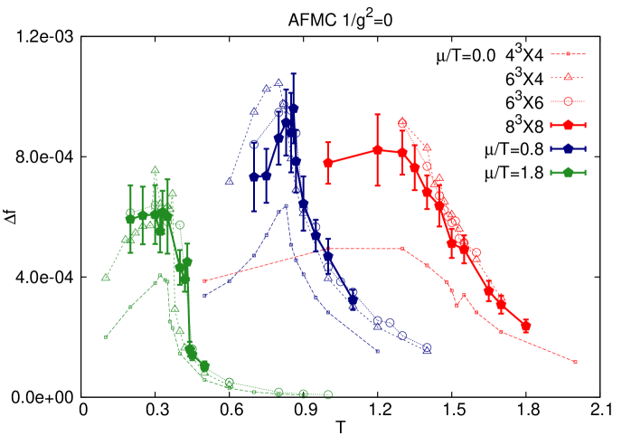
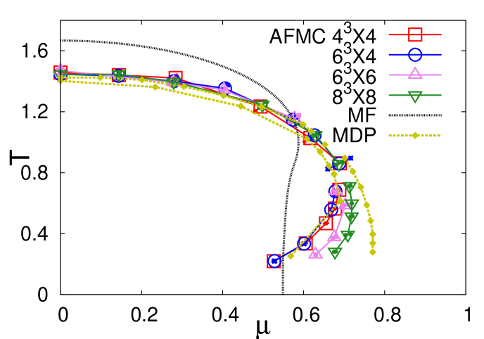
Figure 3: Difference of free energy density between full and phase quenched MC simulations, $\Delta f$, in AFMC as a function of temperature (left panel) and phase boundary (right panel). In left panel, we only show the jack-knife error bars in the results on a $8^{4}$ lattice. In right panel, we show various lattice size results in AFMC. MF denotes the mean field result. MDP is the result based on Monomer-Dimer-Polymer (MDP) simulations [5, 6].

It is important to know how severe the sign problem is in both MDP and AFMC to analyze the QCD phase diagram on a large lattice. The severity of the sign problem is characterized by the difference of the free energy density, $\Delta f=f_{\mathrm{full}}-f_{\mathrm{p.q.}}$, in full Monte-Carlo (MC) and phase quenched MC simulations; $\Delta f$ is related to the average phase factor as $e^{-\Omega\Delta f}=\left<e^{\mathrm{i}\delta}\right>$, where $\Omega$ and $\delta$ are the space-time volume and the complex phase in each configuration, respectively. Comparison of $\Delta f$ in MDP [8] and AFMC (shown in Fig. 3) shows that $\Delta f$ of AFMC is twice as large as that of MDP.

In this paper, we discuss the QCD phase diagram and the mechanism for the sign problem to appear in AFMC, where we integrate out auxiliary fields exactly by using MC technique. We here examine the high momentum auxiliary mode contributions to the weight cancellation and order parameters. These analyses are carried out in the chiral angle fixing (CAF) method, where we fix the chiral angle in each configuration and we can guess an appropriate chiral limit in a large volume. Finally, we give the QCD phase diagram obtained in AFMC with CAF.

2 Formalism

2.1 Effective action & AFMC method

In present article, we consider the case where $SU(N_{c}=3)$ in 3+1 dimension $(d=3)$ space-time. Temporal and spatial lattice sizes are $N_{\tau}$ and $L$. In the strong coupling limit, we can ignore the plaquette term in the lattice QCD action. After integrating out spatial link variables in the leading order of the $1/d$ expansion, the strong coupling limit (SCL) effective action [1, 7, 2, 3, 4, 9] with one species of unrooted staggered fermion is given as,

$$S_{\mathrm{eff}} =\frac{1}{2}\sum_{x}\left[V^{+}_{x}-V^{-}_{x}\right]-\displaystyle\frac{1}{4N_{c}}\sum_{x}M_{x}M_{x+\hat{j}}+m_{0}\sum_{x}M_{x}\ ,$$ (1)

$$V^{+}_{x} =\gamma e^{\mu/\gamma^{2}}\bar{\chi}_{x}U_{0,x}\chi_{x+\hat{0}}\ ,\quad V^{-}_{x}=\gamma e^{-\mu/\gamma^{2}}\bar{\chi}_{x+\hat{0}}U^{\dagger}_{0,x}\chi_{x}\ ,\quad M_{x}=\bar{\chi}_{x}\chi_{x}\ ,$$ (2)

where $\chi_{x}(\bar{\chi}_{x})$ and $U_{\nu,x}$ denote the (anti-)quark field and the link variable. We introduce anisotropic factor $\gamma$ as the ratio of temporal to spatial action coefficients [2, 5, 6, 9, 8], and chemical potential $\mu$ as temporal component of vector potential. $\eta_{j,x}=(-1)^{x_{0}+\cdots+x_{j-1}}$ is the staggered sign factor.

Next, we bosonize 4-fermi like terms to integrate out Grassmann variables. Since mesonic fields ($M_{x}$) take different value at each site, we use the extended Hubbard-Stratonovich (EHS) transformation [4, 7].

$$e^{\alpha AB}=\int\,d\sigma\,d\pi\,e^{-\alpha\left\{\sigma^{2}+\pi^{2}+\sigma(A+B)+i\pi(A-B)\right\}}\ .$$ (3)

Eq. (3) is an identical equation, so it is inevitable that we introduce an imaginary number coefficient. This is the origin of the sign problem in AFMC. After spatial Fourier transformation ($M_{x=(\bm{x},\tau)}=\sum_{\bm{k}}e^{\mathrm{i}\bm{k}\cdot\bm{x}}M_{\bm{k},\tau}$), we utilize the EHS transformation with respect to the eigen value of the composite mesonic fields (the second term of Eq. (1)). Then, the auxiliary fields for $M_{\bm{k},\tau}$ and $\mathrm{i}M_{\bar{\bm{k}},\tau}$ ($\bar{\bm{k}}=\bm{k}+(\pi,\pi,\pi)$) are introduced as $\sigma_{-\bm{k}}$ and $\pi_{\bm{k}}$ [7]. After bosonization, the action becomes

$$S_{\mathrm{eff}}^{\mathrm{EHS}} =\frac{1}{2}\sum_{x}\left[V_{x}^{+}-V_{x}^{-}\right]+\sum_{x}m_{x}M_{x}+\frac{L^{3}}{4N_{c}}\sum_{{{\mathbb{k}},\tau},f({\mathbb{k}})>0}f({\mathbb{k}})\left[\left|\sigma_{{\mathbb{k}},\tau}\right|^{2}+\left|\pi_{{\mathbb{k}},\tau}\right|^{2}\right]\ ,$$ (4)

$$m_{x} =m_{0}+\frac{1}{4N_{c}}\sum_{j}\left[(\sigma+i\varepsilon\pi)_{x+\hat{j}}+(\sigma+i\varepsilon\pi)_{x-\hat{j}}\right]\ ,$$ (5)

where $f(\bm{k})=\sum_{j=1}^{d}\cos k_{j}$, $\sigma_{x}=\sum_{{\mathbb{k}},f({\mathbb{k}})>0}e^{i\mathbb{k}\cdot\mathbb{x}}\sigma_{{\mathbb{k}},\tau}$, and $\pi_{x}=\sum_{{\mathbb{k}},f({\mathbb{k}})>0}(-1)^{\tau}e^{i\mathbb{k}\cdot\mathbb{x}}\pi_{{\mathbb{k}},\tau}$. $\varepsilon_{x}=(-1)^{x_{0}+\cdots+x_{3}}$ plays a similar role to $\gamma_{5}$ in the continuum limit. We should notice that the imaginary number exists in the spatial diagonal parts of the fermion matrix from the modified mass terms.

Finally, we integrate out the Grassmann and temporal link ($U_{0}$) variables analytically [9], and obtain the effective action,

$$S_{\mathrm{eff}}^{\mathrm{AF}}=\sum_{{{\mathbb{k}},\tau},f({\mathbb{k}})>0}\frac{L^{3}f({\mathbb{k}})}{4N_{c}}\left[\left|\sigma_{{\mathbb{k}},\tau}\right|^{2}+\left|\pi_{{\mathbb{k}},\tau}\right|^{2}\right]-\sum_{\bm{x}}\log\left[X_{N_{\tau}}(\mathbb{x})^{3}-2X_{N_{\tau}}(\mathbb{x})+2\cosh(\frac{3N_{\tau}\mu}{\gamma^{2}})\right]\ .$$ (6)

$X_{N_{\tau}}$ is a function of the modified mass ($m_{x}$), and obtained by using a recursion formula[9]. In the MF approximation, we get $X_{N_{\tau}}=2\cosh(N_{\tau}\mathrm{arcsinh}(m_{x}/\gamma))$. We numerically carry out the auxiliary field ($\sigma_{\mathbf{k},\tau},\pi_{\mathbf{k},\tau}$) integration of the partition function, $Z=\int\mathcal{D}[\sigma,\pi]\exp(-S_{\mathrm{eff}}^{\mathrm{AF}})$, by using the Monte-Carlo method.

2.2 Weight cancellation in AFMC

We have the weight cancellation since the complex phase in $\exp(-S_{\mathrm{eff}}^{\mathrm{AF}})$ appears from $X_{N_{\tau}}$via complex $m_{x}$. For low-momentum modes, the phase cancellation mechanism exists and the weight cancellation is not severe [7]. An imaginary part in the modified mass term involves $\varepsilon_{x}$. In the case where the $\pi$ fields take a constant amplitude, the imaginary contribution from one site in Eq. (6) cancels with that in the nearest neighbor site contribution. Then we expect that the weight cancellation is not severe as long as low momentum modes contribute. By comparison, we may have the severe weight cancellation when high momentum modes dominate. In Sec. 3, we quantitatively confirm these high momentum contributions.

2.3 Chiral Angle Fixing

We develop a way to define the chiral condensate and the chiral susceptibility on a finite volume lattice in the chiral limit. Since the chiral transformation mixes the scalar mode, $\sigma_{0}$ $=\sum_{\tau}\sigma_{\bm{k}=0,\tau}/N_{\tau}$, and its chiral partner, the pseudoscalar mode, $\pi_{0}=\sum_{\tau}(-1)^{\tau}\pi_{\bm{k}=0,\tau}/N_{\tau}$, as

$$\left(\begin{array}[]{c}\sigma_{0}^{\prime}\\ \pi_{0}^{\prime}\end{array}\right)=\left(\begin{array}[]{cc}\cos\alpha&\sin\alpha\\ -\sin\alpha&\cos\alpha\end{array}\right)\left(\begin{array}[]{c}\sigma_{0}\\ \pi_{0}\end{array}\right),$$ (13)

the order parameter $\left<\sigma_{0}\right>$ vanishes on a finite size lattice in the chiral limit. Rigorously, we need to take the thermodynamic limit followed by $m_{0}\to 0$ as shown in Fig. 1, then we obtain finite $\left<\sigma_{0}\right>$ and zero $\left<\pi_{0}\right>$. This procedure is time-comsuming, and the root mean square order parameter is adopted to avoid these problems in spin systems [10]. We here propose a similar method, Chiral Angle Fixing (CAF). In order to get the appropriate chiral condensate in the chiral limit, we rotate $\sigma_{0}$ and $\pi_{0}$ onto the $\sigma_{0}$ axis. Other auxiliary fields are also rotated by $\alpha$ as in Eq. (13) in each Monte-Carlo configuration, where $\alpha=\arctan(\pi_{0}/\sigma_{0})$. We use these new fields to obtain the order parameters and other quantities.

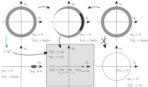
Figure 1: Schematic picture of CAF method. In order to obtain the value of chiral condensate, we put a finite mass, first take thermodynamic limit and finally take the chiral (massless) limit (like center bottom figure). In CAF, we take chiral rotation to make the $\pi_{0}$ field disappears. Then, we get the finite chiral condensate (left bottom figure), which would be close to the correct value.

We consider CAF from a different point of view. Chiral condensate is described by

$$\left<\sigma_{0}\right> = \frac{1}{Z}\int\mathcal{D}\left[\sigma_{0},\pi_{0}\right]\ \prod_{(\mathbf{k},\omega)\not=(\bm{0},0)}\mathcal{D}\left[\sigma_{\mathbf{k},\omega},\pi_{\mathbf{k},\omega}\right]\ \sigma_{0}\ e^{-S(\sigma_{\mathbf{k},\omega},\pi_{\mathbf{k},\omega},\phi=\sqrt{\sigma_{0}^{2}+\pi_{0}^{2}},\alpha)}\$$ (14)

$$= \frac{1}{Z}\int\mathcal{D}\left[\phi,\alpha\right]\ \phi\cos\alpha\prod_{(\mathbf{k},\omega)\not=(\bm{0},0)}\int\mathcal{D}\left[\phi_{\mathbf{k},\omega},\alpha_{\mathbf{k},\omega}^{\prime}\right]\ e^{-S(\phi_{\mathbf{k},\omega},\alpha_{\mathbf{k},\omega}^{\prime},\phi,0)}=0,$$

where we define $\sigma_{\mathbf{k},\omega},\ \pi_{\mathbf{k},\omega}$ as the Fourier transform of auxiliary fields other than $\sigma_{0},\pi_{0}$ modes. $\phi_{\mathbf{k},\omega}$ and $\alpha_{\mathbf{k},\omega}$ are chiral radius and chiral angle in regard to each chiral partner, respectively. We also use a relation, $S(\phi_{\mathbf{k},\omega},\alpha_{\mathbf{k},\omega},\phi,\alpha)=S(\phi_{\mathbf{k},\omega},\alpha_{\mathbf{k},\omega}^{\prime}=\alpha_{\mathbf{k},\omega}-\alpha,\phi,0)$. According to Eq. (14), chiral condensate is identically equal to zero. After we take CAF method, we fix $\alpha$ to $\sigma_{0}$ axis and $\pi_{0}=0$. We obtain finite chiral condensate

$$\left<\sigma_{0}\right>=\frac{1}{Z}\int\mathcal{D}\sigma_{0}\ \sigma_{0}\prod_{(\mathbf{k},\omega)\not=(\bm{0},0)}\int\mathcal{D}\left[\phi_{\mathbf{k},\omega},\alpha_{\mathbf{k},\omega}\right]\ \ e^{-S(\phi_{\mathbf{k},\omega},\alpha_{\mathbf{k},\omega},\phi=\sigma_{0},0)}\neq 0,$$ (15)

in the Nambu-Goldstone (NG) phase. We eventually obtain chiral condensate and chiral susceptibility with finite peak. Chiral condensate obtained in CAF should mimic the spontaneous chiral condensate in the thermodynamic limit.

3 Results of high momentum mode contributions

We show the numerical results in this section, where we have assumed $T=\gamma^{2}/N_{\tau}$ [2]. All results are carried out under CAF method, and error bars are estimated by the jack-knife method. We quantitatively confirm high momentum auxiliary field mode contributions to the average phase factor $\left<e^{\mathrm{i}\delta}\right>$ and the order parameters. We cut off high momentum modes with the squared spatial momentum of auxiliary fields ($\sum_{j=1}^{d}\sin^{2}k_{j}$) more than the parameter $\Lambda$, and examine their effects. The parameter $\Lambda$ runs from 0 through $d=3$. When $\Lambda$ is equal to 3, we consider all Monte-Carlo configurations. By comparison, we only include the lowest momentum modes when $\Lambda$ is equal to 0.

Figure 2: Cut-off parameter $\Lambda$ dependence of average phase factor (left top), quark number density (left bottom), chiral susceptibility (right top), quark number susceptibility (right middle), and chiral condensate (right bottom) as a function of temperature on a $8^{4}$ lattice in the chiral limit for fixed $\mu/T=0.6$.

As discussed in Sec. 2, the phase cancellation might be severe when high momentum modes contribute to the effective action. We could expect that the weight cancellation becomes weaker if we cut off the high momentum modes. In Fig. 2, we show the average phase factor on a $8^{4}$ lattice for fixed $\mu/T=0.6$ in the chiral limit. We find that the weight cancellation weakens when $\Lambda$ goes to 0. This is consistent with our consideration of the phase cancellation with low momentum modes, and we could conclude that high momentum modes lead to strong weight cancellation.

We show the chiral condensate after CAF in the right bottom panel of Fig. 2. The behavior of the chiral condensate does not depend on the cut-off parameter $\Lambda$. This is because integration variables in AFMC are the mesonic auxiliary fields ($\sigma_{\mathbf{k},\tau},\pi_{\mathbf{k},\tau}$), and the scalar and pseudoscalar modes are comprised of the lowest modes of the integration variables. In Fig. 2, we also plot the cut-off dependence of quark number density, chiral susceptibility and quark number susceptibility. These results demonstrate that no cut-off dependence as long as the parameter $\Lambda$ is larger than 2. Revisiting the average phase factor, we know the statistical weight cancellation weakens in cases where $\Lambda$ is less than 2.5. Therefore, these results indicate that there exists a optimal cut-off $\Lambda_{o}$, where the behavior of the order parameters does not change and we could improve the reliability of numerical simulation. There is a possibility to investigate the QCD phase diagram on a larger lattice by cutting off or approximating the high momentum modes without changing the behavior of order parameters.

Finally, we show the results of the chiral phase transition by using CAF. The order of the chiral phase transitions are deduced from the distribution of chiral condensate instead of considering finite size scaling of chiral susceptibility due to small lattice size[7]. The distribution analysis indicates that the order of transition is the 1st (2nd or cross-over) order at high (low) $\mu$. We deduce the would-be 1st order phase boundary as the point where the minimum of the effective potential changes discontinuously. We obtain the would-be 2nd order phase boundary by fitting the peak of chiral susceptibility with the quadratic function. The error bars include both statistical and systematic errors for the (would-be) 2nd order transition. The present phase boundary is consistent with Monomer-Dimer-Polymer (MDP) simulation result [5, 6]. Both results show the NG phase is suppressed at low $\mu$ and broadened at high $\mu$ compared to the mean field (MF) results. In high $\mu$ region, the NG phase is enlarged as the temporal lattice size $N_{\tau}$ becomes large. This behavior is also seen in MDP, which is also extrapolated to $N_{\tau}\rightarrow\infty$.

4 Summary

We have discussed the mechanism for the sign problem to appear in the auxiliary field Monte-Carlo (AFMC) method based on an effective action, $S_{\mathrm{eff}}^{\mathrm{AF}}$. The root cause of the sign problem in AFMC is extended Hubbard-Stratonovich (EHS) transformation, since we must introduce complex terms in bosonization. The complex terms in the effective action is eventually in the spatial diagonal parts of the fermion matrix (the modified mass terms). The statistical weight cancellation arises when we numerically integrate out auxiliary fields on the basis of $S_{\mathrm{eff}}^{\mathrm{AF}}$. We quantitatively confirm that the high momentum modes contribute to the weight cancellation. We also give a new approach respecting chiral symmetry named as the Chiral Angle Fixing (CAF) method. We rotate all auxiliary field modes in each Monte-Carlo configuration by fixing the chiral angle, the angle between the scalar and the pseudoscalar modes, to zero. We acquire the finite chiral condensate and the chiral susceptibility with a peak respecting chiral symmetry in CAF. Finally, we find that the chiral phase transition boundary in CAF is consistent with another method called Monomer-Dimer-Polymer (MDP) simulations [5, 6].

5 Acknowledgement

TI is supported by Grants-in-Aid for the Japan Society for Promotion of Science (JSPS) Research Fellows (No. 25-2059). This work was supported in part by Grants-in-Aid for Scientific Research from the Japan Society for the Promotion of Science (JSPS) (Nos. 23340067, 24340054, 24540271), by Grant-in-Aid for Innovative Areas from the Ministry of Education, Culture, Sports, Science and Technology of Japan (MEXT) (Area No. 2404, Nos. 24105001, 24105008), by the Yukawa International Program for Quark-Hadron Sciences.

References

- [1] H. Kluberg-Stern, A. Morel, O. Napoly, and B. Petersson, Nucl. Phys. B 190, 504 (1981); N. Kawamoto and J. Smit, Nucl. Phys. B 192, 100 (1981); T. Jolicoeur, H. Kluberg-Stern, M. Lev, A. Morel, and B. Petersson, Nucl. Phys. B 235, 455 (1984); P. H. Damgaard, N. Kawamoto, and K. Shigemoto, Phys. Rev. Lett 53, 2211 (1984).
- [2] N. Bilic, F. Karsch, and K. Redlich, Phys. Rev. D 45, 3228 (1992).
- [3] Y. Nishida, Phys. Rev. D 69, 094501 (2004); K. Fukushima, Prog. Theor. Phys. Supplement 153, 204 (2004).
- [4] K. Miura, T. Z. Nakano, A. Ohnishi, and N. Kawamoto, Phys. Rev. D 80, 074034 (2009); T. Z. Nakano, K. Miura, and A. Ohnishi, Prog. Theor. Phys. 123, 825 (2010).
- [5] P. de Forcrand and M. Fromm, Phys. Rev. Lett. 104, 112005 (2010).
- [6] W. Unger and P. de Forcrand, J. Phys. G 38, 124190 (2011).
- [7] A. Ohnishi, T. Ichihara, and T. Z. Nakano, PoS LATTICE2012, 088 (2012).
- [8] M. Fromm, Lattice QCD at strong coupling: thermodynamics and nuclear physics, PhD thesis, Eidgenssische Technische Hochschule ETH Zrich, (2010).
- [9] G. Fldt and B. Petersson, Nucl. Phys. B 265, 197 (1986); N. Bilic, K. Demeterfi, and B. Petersson, Nucl. Phys. B 377, 651 (1992).
- [10] B. Kurt and W. H. Dieter, Monte Carlo simulation in statistical physics: an introduction (Springer Verlag, Berlin, 2010), References therein.