Randall-Sundrum scenario with a small curvature and Drell-Yan process at the LHC

Abstract

The Randall-Sundrum-like scenario with the small curvature $\kappa$ (RSSC model) is studied in detail in comparison with the original RS1 model. In the framework of the RSSC model, the $p_{\perp}$ distributions for the dilepton production at the LHC are calculated. Both dielectron and dimuon events are taken into account. The important feature of calculations is the account of the widths of massive graviton excitations. For the summary statistics taken at 7 TeV ($L=5\ \mathrm{fb}^{-1}$) and 8 TeV ($L=20\ \mathrm{fb}^{-1}$), the exclusion limit on the 5-dimensional gravity scale $M_{5}$ is set to be 6.84 TeV at 95$\%$ C.L. For $\sqrt{s}=13$ TeV and integrated luminosity 30 fb^-1, the LHC search limit is found to be 10.16 TeV. These bounds on $M_{5}$ are independent of $\kappa$ (up to powerlike corrections), provided $\kappa\ll M_{5}$.

1 Randall-Sunrum scenario with the small
curvature (RSSC model)

In a recent paper [1], the $p_{\perp}$ distributions for dimuon production at the LHC were calculated in the framework of the Randall-Sundrum-like scenario with a small curvature (RSSC model, in what follows). The LHC discovery limits on 5-dimensional gravity scale $M_{5}$ were obtained for both 7 TeV and 14 TeV. In the present paper, the combined analysis of both dielectron and dimuon events at 7, 8, and 13 TeV will be done.

Before presenting results of calculations for the Drell-Yan (DY) process at the LHC, it is useful to compare the RSSC model with the standard Randall-Sundrum model with two 3D branes (RS1 model [2]). The classical action of this scenario is given by

$$S =2\bar{M}_{5}^{3}\int\!\!d^{4}x\!\!\int_{-\pi r_{c}}^{\pi r_{c}}\!\!dy\,\sqrt{|G|}\,(\mathcal{R}-\Lambda)$$

$$+\int\!\!d^{4}x\sqrt{|g^{(1)}|}\,(\mathcal{L}_{1}-2\bar{M}_{5}^{3}\Lambda_{1})+\int\!\!d^{4}x\sqrt{|g^{(2)}|}\,(\mathcal{L}_{2}-2\bar{M}_{5}^{3}\Lambda_{2})\;,$$ (1)

where $G_{MN}(x,y)$ is the 5-dimensional metric, with $M,N=\{\mu,4\}$; $\mu=0,1,2,3$; $y$ is the 5-th dimension coordinate; and $r_{c}$ is the size of the ED. The quantities

$$g^{(1)}_{\mu\nu}(x)=G_{\mu\nu}(x,y=0)\;,\quad g^{(2)}_{\mu\nu}(x)=G_{\mu\nu}(x,y=\pi r_{c})$$ (2)

are induced metrics on the branes, and $\mathcal{L}_{1}$ and $\mathcal{L}_{2}$ are brane Lagrangians. It is assumed that the cosmological constant $\Lambda$ is negative. Thus, we have a slice of the AdS₅ space-time.

In Ref. [2] the background warped metric was found to be

$$\mathrm{RS1}:\quad ds^{2}=e^{-2\kappa|y|}\,\eta_{\mu\nu}\,dx^{\mu}\,dx^{\nu}-dy^{2}\;,$$ (3)

where $\eta_{\mu\nu}$ is the Minkowski tensor with the signature $(1,-1,-1,-1)$. The periodicity $y=y+2\pi r_{c}$ is imposed and the points $(x_{\mu},y)$ and $(x_{\mu},-y)$ are identified. So, one gets the orbifold $S^{1}\!/Z_{2}$.

In the RS1 model the 3D branes are located at the fixed points $y=0$ (Plank brane) and $y=\pi r_{c}$ (TeV brane). The SM fields are constrained to the TeV brane, while the gravity propagates in all spatial dimensions.

The hierarchy relation between the 5-dimensional reduced gravity scale $\bar{M}_{5}$ and reduced Planck mass $\bar{M}_{\mathrm{Pl}}$ looks like [2],

$$\mathrm{RS1}:\quad\bar{M}_{\mathrm{Pl}}^{2}=\frac{\bar{M}_{5}^{3}}{\kappa}\left(1-e^{-2\pi\kappa r_{c}}\right)\;.$$ (4)

The reduced scales in (4) are defined as follows

$$\bar{M}_{\mathrm{Pl}}=M_{\mathrm{Pl}}/\sqrt{8\pi}\simeq 0.20\,M_{\mathrm{Pl}}\simeq 2.4\cdot 10^{18}\ \mathrm{GeV}\;,$$ (5)

$$\bar{M}_{5}=M_{5}/(2\pi)^{1/3}\simeq 0.54\,\bar{M}_{5}\;.$$ (6)

The warp factor $F=\exp(-2\kappa|y|)$ has the following values on the branes

$$\mathrm{RS1}:\quad F\Big{|}_{y=0}=1\;,\quad F\Big{|}_{y=\pi r_{c}}=e^{-2\pi\kappa r_{c}}\;.$$ (7)

For $\kappa>0$, we get for boundary cosmological terms

$$\mathrm{RS1}:\quad\Lambda_{1}>0\;,\quad\Lambda_{2}<0\;.$$ (8)

Thus, the Planck brane has a positive tension, while the TeV brane has a negative tension.

In order for the hierarchy relation (4) to be satisfied, one has to put

$$\mathrm{RS1}:\quad\kappa\sim\bar{M}_{5}\sim M_{\mathrm{Pl}}\;.$$ (9)

The RS1 model predicts a series of massive Kaluza-Klein (KK) graviton resonances with the lightest graviton about 1 TeV.

After the replacement

$$\kappa\rightarrow-\kappa\;,$$ (10)

the RS1 metric becomes [3]

$$ds^{2}=e^{2\kappa|y|}\,\eta_{\mu\nu}\,dx^{\mu}\,dx^{\nu}-dy^{2}\;.$$ (11)

The hierarchy relation is modified as follows

$$\bar{M}_{\mathrm{Pl}}^{2}=\frac{\bar{M}_{5}^{3}}{\kappa}\left(e^{2\pi\kappa r_{c}}-1\right)\;.$$ (12)

The warp factor $F=\exp(2\kappa|y|)$ and brane cosmological terms acquire the meanings

$$F\Big{|}_{y=0}=1\;,\quad F\Big{|}_{y=\pi r_{c}}=e^{2\pi\kappa r_{c}}\;,$$ (13)

$$\Lambda_{1}<0\;,\quad\Lambda_{2}>0\;.$$ (14)

Thus, after replacement (10) the branes are interchanged. The brane $y=0$ becomes the TeV brane on which all the SM fields live. The ratio of the warp factors remains the same (namely, $\exp(2\pi\kappa r_{c})$), but the very value of the warp factor on the TeV brane becomes equal to unity.

In such a scheme, $\bar{M}_{5}$ can be one to tens TeV, while the curvature $\kappa$ is allowed to vary from hundred MeV to tens GeV [3, 4]. The masses of the KK gravitons are proportional to the curvature $\kappa$ (see below Eq. (47)).

Note that after changing variables in (3)

$$x^{\mu}\rightarrow x^{\prime\mu}=e^{-\pi\kappa r_{c}}\,x^{\mu}\;,$$ (15)

one obtains the metric [4, 5]

$$\quad ds^{2}=e^{2\kappa(\pi r_{c}-|y|)}\eta_{\mu\nu}\,dx^{\prime\mu}\,dx^{\prime\nu}-dy^{2}\;,$$ (16)

which also leads to the modified hierarchy relation (12).

The metric with the small curvature, which takes into account the orbifold structure of the space-time, looks like (for details, see Appendix A)

$$\mathrm{RSSC}:\quad ds^{2}=e^{-2\sigma(y)}\eta_{\mu\nu}\,dx^{\mu}\,dx^{\nu}-dy^{2}\;,$$ (17)

with

$$\sigma(y)=\frac{\kappa}{2}\,(|y|-|\pi r_{c}-y|-\pi r_{c})\;,$$ (18)

Note that the metrics (16) and (17) coincide for $0<y<\pi r_{c}$.

The warp factor $F=\exp[-2\sigma(y)]$ with the RSSC function $\sigma(y)$ (18) has the following values at the fixed points

$$\mathrm{RSSC}:\quad F\Big{|}_{y=0}=e^{2\pi\kappa r_{c}}\;,\quad F\Big{|}_{y=\pi r_{c}}=1\;.$$ (19)

The boundary cosmological terms are

$$\mathrm{RSSC}:\quad\Lambda_{1}>0\;,\quad\Lambda_{2}<0\;.$$ (20)

The hierarchy relation,

$$\mathrm{RSSC}:\quad\bar{M}_{\mathrm{Pl}}^{2}=\frac{\bar{M}_{5}^{3}}{\kappa}\left(e^{2\pi\kappa r_{c}}-1\right)\;,$$ (21)

is the same as Eq. (12). In order for relation (21) to be satisfied, it is enough to take $\kappa r_{c}\approx 10$.

In between the branes, the 5-dimensional scalar curvature is negative,

$$\mathcal{R}_{5}=-20\kappa^{2}\;,$$ (22)

while the radius of the curvature is equal to $\kappa^{-1}$ (see Appendix A).

Let us use a linear expansion of the metric about its Minkowski value (see, for instance, [6])

$$G_{\mu\nu}=e^{-2\sigma}\!\bigg{(}\eta_{\mu\nu}+\frac{1}{M_{5}^{3/2}}\,H_{\mu\nu}\bigg{)}\;,\quad G_{44}=-1+H_{44}\;.$$ (23)

After redefinition $H_{\mu\nu}=h_{\mu\nu}+H_{44}/2$, where $H_{44}=2\,e^{2\sigma}\phi(x)$ [7], and imposing transverse-traceless gauge,

$$\partial^{\mu}h_{\mu\nu}=0\;,\quad h_{\mu}^{\mu}=0\;,$$ (24)

the metric fluctuation $h_{\mu\nu}$ describes the massive spin-2 field with 5 degrees of freedom. It can be decomposed into KK graviton excitations

$$h_{\mu\nu}(x,y)=\frac{1}{\sqrt{2\pi r_{c}}}\sum_{n=0}^{\infty}h_{\mu\nu}^{(n)}(x)\,\psi^{(n)}(y)\;.$$ (25)

The wave functions of the KK excitations obey the equation [6]

$$\frac{d}{dy}\!\left(e^{-4\sigma(y)}\frac{d}{dy}\right)\psi^{(n)}(y)=-m_{n}^{2}\,e^{-2\sigma(y)}\,\psi^{(n)}(y)\;,$$ (26)

with $m_{n}$ being the mass of four-dimensional gravitons,

$$(\eta^{\mu\nu}\partial_{\mu}\partial_{\nu}+m_{n}^{2})h_{\mu\nu}^{(n)}(x)=0\;.$$ (27)

Equation (26) follows from 4-dimensional components of the Einstein-Hilbert equation, if one keeps only linear terms in $h_{\mu\nu}$. Note that Eq. (26) means that

$$\square_{5}h_{\mu\nu}(x,y)=0\;,$$ (28)

where $\square_{5}$ is the 5-dimensional d’Alembertian in the background metric (17).

The eigenfunctions $\psi^{(n)}(y)$ satisfy the boundary conditions

$$\frac{d\psi^{(n)}}{dy}\Big{|}_{y=0}=0\;,$$ (29)

$$\frac{d\psi^{(n)}}{dy}\Big{|}_{y=\pi r_{c}}=0\;,$$ (30)

as well as the orthonormality condition

$$\frac{1}{\pi r_{c}}\int_{0}^{\pi r_{c}}\!\!\!dy\,e^{-2\sigma(y)}\,\psi^{(n)}(y)\,\psi^{(m)}(y)=\delta_{nm}\;.$$ (31)

Thus, we have the Sturm-Liouville problem (26), (29)-(31).

To solve it, let us put for $n>0$

$$\psi^{(n)}(y)=z_{n}^{2}\phi^{(n)}(z_{n})\;,$$ (32)

where

$$z_{n}=z_{n}(y)=\frac{m_{n}}{\kappa}\,e^{\sigma(y)}\;.$$ (33)

Then we get from (26)

$$\bigg{[}z_{n}^{2}(\phi^{(n)}(z_{n}))^{\prime\prime}+z_{n}(\phi^{(n)}(z_{n}))^{\prime}+(z_{n}^{2}-4)\phi^{(n)}(z_{n})\bigg{]}\left(\frac{\sigma^{\prime}}{\kappa}\right)^{2}$$

$$+ \bigg{[}z_{n}(\phi^{(n)}(z_{n}))^{\prime}+2\phi^{(n)}(z_{n})\bigg{]}\frac{\sigma^{\prime\prime}}{\kappa^{2}}=0\;.$$ (34)

Here and in what follows the prime denotes the derivative with respect to variable $y$.

The solution of Eq. (1) which satisfies the right boundary condition (30) is given in terms of Bessel functions

$$\phi^{(n)}(y)=C_{n}[J_{2}(z_{n})Y_{1}(b_{n})-Y_{2}(z_{n})J_{1}(b_{n})]\;,$$ (35)

where

$$b_{n}=\frac{m_{n}}{\kappa}\;,$$ (36)

and $C_{n}$ is a constant.

The left boundary condition (29) defines the masses of the KK gravitons with respect to the TeV brane. Taking into account that $\sigma(0)=-\kappa\pi r_{c}$, we get

$$J_{1}(a_{n})Y_{1}(b_{n})-Y_{1}(a_{n})J_{1}(b_{n})=0\;,$$ (37)

where

$$a_{n}=\frac{m_{n}}{\kappa}\,e^{-\kappa\pi r_{c}}\;.$$ (38)

Let us demonstrate that the second term in (1) is equal to zero. Indeed, by using relation $xZ_{2}^{\prime}(x)+2Z_{2}(x)=xZ_{1}(x)$, where $Z_{\nu}=J_{\nu}$ or $Y_{\nu}$, it can be presented in the form

$$\frac{C_{n}}{\kappa}\,[J_{1}(z_{n})Y_{1}(b_{n})-Y_{1}(z_{n})J_{1}(b_{n})][\delta(y)-\delta(y-\pi r_{c})]\;.$$ (39)

Note that

$$z_{n}(y)=\left\{\begin{array}[]{ll}a_{n},&y=0\\ b_{n},&y=\pi r_{c}\end{array}\right.$$ (40)

Thus, the expression in (39) vanishes due to the boundary condition (37).

As a result, we obtain for $n>0$

$$\psi^{(n)}(y)=N_{n}e^{2\sigma}\,[J_{2}(z_{n})Y_{1}(b_{n})-Y_{2}(z_{n})J_{1}(b_{n})]\;,$$ (41)

where the normalization constant $N_{n}$ is defined from the orthonormality condition (31). An explicit form of $N_{n}$ is derived in Appendix B.

As for the zero mode excitation, its wave function looks like

$$\psi^{(0)}(y)=N_{0}=\left(\frac{2\pi\kappa r_{c}}{e^{2\pi\kappa r_{c}}-1}\right)^{\!1/2}=\sqrt{2\pi r_{c}}\,\,\frac{\bar{M}_{5}^{3/2}}{\bar{M}_{\mathrm{Pl}}}\;.$$ (42)

The orthogonality of the zero mode (42) and KK modes (41) comes from the equation ($n>0$)

$$\int_{0}^{\pi r_{c}}\!\!\! dy\,e^{-2\sigma(y)}\,\psi^{(0)}(y)\,\psi^{(n)}(y)=\frac{N_{0}N_{n}}{\kappa}\int_{a_{n}}^{b_{n}}\frac{dz}{z}\,[J_{2}(z)Y_{1}(b_{n})-Y_{2}(z)J_{1}(b_{n})]$$

$$=\frac{N_{0}N_{n}}{a_{n}\kappa}[J_{1}(a_{n})Y_{1}(b_{n})-Y_{1}(a_{n})J_{1}(b_{n})]=0\;.$$ (43)

The interactions of massless gravitons on the TeV brane are given by the Lagrangian

$$\mathcal{L}_{\mathrm{int}}^{(0)} =-\frac{1}{\bar{M}_{5}^{3/2}}\int\!\!dy\,h_{\mu\nu}^{(0)}(x,y)\,T^{\mu\nu}(x)\delta(y-\pi\kappa r_{c})$$

$$=-\frac{1}{\bar{M}_{\mathrm{Pl}}}h_{\mu\nu}^{(0)}(x)\,T^{\mu\nu}(x)\;,$$ (44)

where $T^{\mu\nu}(x)$ is the energy-momentum tensor of the SM fields.

Let us consider Eq. (37) in more detail. Since

$$\frac{e^{-\kappa\pi r_{c}}}{\kappa}\simeq\frac{1}{\bar{M}_{\mathrm{Pl}}}\left(\frac{\bar{M}_{5}}{\kappa}\right)^{3/2}\!\ll 1\;,$$ (45)

$m_{n}$ are defined by the equation

$$J_{1}(b_{n})=0\;.$$ (46)

As a result, the graviton masses have appeared to be proportional to $\kappa$,

$$m_{n}=x_{n}\kappa\;,\quad n=1,2,\ldots\;,$$ (47)

where $x_{n}$ are zeros of the Bessel function $J_{1}(x)$.

In the limit of a very small curvature,

$$2\pi\kappa r_{c}\ll 1\;,$$ (48)

one can use asymptotic values of the Bessel functions

$$J_{1}(z) =\sqrt{\frac{2}{\pi z}}\left[\sin\left(z-\frac{\pi}{4}\right)+\mathrm{O}(|z|^{-1})\right]\;,$$

$$Y_{1}(z) =-\sqrt{\frac{2}{\pi z}}\left[\cos\left(z-\frac{\pi}{4}\right)+\mathrm{O}(|z|^{-1})\right]\;.$$ (49)

Then we get from (37)

$$\sin(b_{n}-a_{n})\simeq\,\sin(\pi r_{c}m_{n})=0\;,$$ (50)

that results in the well-known graviton spectrum in the model with one flat ED [9]-[11]

$$m_{n}=\frac{n}{r_{c}}\;,\quad n=1,2,\ldots\;.$$ (51)

As one can see, $a_{n},b_{n}\simeq n/(\kappa r_{c})\gg 1$. Thus, using asymptotic expressions (1) was fully justified.

Let us stress, however, that the AdS₅ space becomes indistinguishable from a five-dimensional flat space only for negligible values of the curvature $\kappa$. Indeed, in the limit (48), Eq. (21) transforms into the hierarchy relation for the flat ED

$$\bar{M}_{\mathrm{Pl}}^{2}=\bar{M}_{5}^{3}(2\pi r_{c})=\bar{M}_{5}^{3}\,V_{1}\;,$$ (52)

where $V_{1}$ is the volume of the compact ED. Then the inequality $2\pi r_{c}\ll\kappa^{-1}$ means

$$\kappa\ll\frac{\bar{M}_{5}^{3}}{\bar{M}_{\mathrm{Pl}}^{2}}\simeq 0.17\cdot 10^{-18}\left(\frac{\bar{M}_{5}}{1\,\mathrm{TeV}}\right)^{3}\mathrm{eV}\;.$$ (53)

The Newton potential between two test masses in the RSSC model was estimated in [12]

$$V(r)=G_{N}\,\frac{m_{1}m_{2}}{r}\left(1+\frac{e^{-m_{1}r}}{\pi\kappa r}\right)\;,$$ (54)

where $m_{1}=x_{1}\kappa$ is the mass of the lightest KK graviton, $x_{1}=3.84$ being the first zero of the Bessel function $J_{1}(x)$. Thus, relative corrections to the Newton law appear to be negligible [12].

The interaction of the massive KK gravitons with the the SM fields on the TeV brane is described by the Lagrangian [3]-[8] (see also [5])

$$\mathcal{L}_{\mathrm{TeV}} =-\frac{1}{\bar{M}_{5}^{3/2}}\sum_{n=1}^{\infty}\int\!\!dy\,\sqrt{G}\,h_{\mu\nu}^{(n)}(x,y)\,T_{\alpha\beta}(x)\,g^{\mu\alpha}g^{\nu\beta}\delta(y-\pi\kappa r_{c})$$

$$=-\frac{1}{\Lambda_{\pi}}\,T_{\alpha\beta}(x)\sum_{n=1}^{\infty}h^{(n)}_{\mu\nu}(x)\,\eta^{\mu\alpha}\eta^{\nu\beta}\;.$$ (55)

The parameter

$$\Lambda_{\pi}=M_{\mathrm{Pl}}\,\sqrt{\frac{1-Y_{1}^{2}(b_{n})/Y_{1}^{2}(a_{n})}{e^{2\kappa\pi r_{c}}-1}}\simeq\bar{M}_{\mathrm{Pl}}\,e^{-\pi\kappa r_{c}}$$ (56)

has the meaning of the physical scale on the TeV brane.

In a number of papers (see, for instance, Refs. [8], [13]), the linear expansion about the background metric,

$$G_{\mu\nu}=e^{-2\sigma}\eta_{\mu\nu}+\frac{1}{M_{5}^{3/2}}\,\tilde{H}_{\mu\nu}\;,\quad G_{44}=-1+H_{44}\;.$$ (57)

is used instead of expansion (23). In such a case, $\tilde{h}_{\mu\nu}=e^{-2\sigma}h_{\mu\nu}$, and the eigenvalue functions are equal to

$$\tilde{\psi}^{(0)}(y) =N_{0}\,e^{-2\sigma(y)}\;,$$ (58)

$$\tilde{\psi}^{(n)}(y) =N_{n}\,[J_{2}(z_{n})Y_{1}(b_{n})-Y_{2}(z_{n})J_{1}(b_{n})]\;,$$ (59)

with the constants $N_{0}$ and $N_{n}$ defined above. The eigenvalue functions obey the following equations

$$\left[\frac{d^{2}}{dy^{2}}-4\sigma^{\prime\,2}(y)+2\sigma^{\prime\prime}(y)\right]\tilde{\psi}^{(n)}(y)=-m_{n}^{2}e^{2\sigma(y)}\tilde{\psi}^{(n)}(y)$$ (60)

and boundary conditions

$$\left[\frac{d}{dy}+2\sigma^{\prime}(y)\right]\tilde{\psi}^{(n)}(y)=0\;,\quad\mathrm{for\ }y=0,\,\pi r_{c}\;.$$ (61)

Correspondingly, the orthonormality condition looks like

$$\frac{1}{\pi r_{c}}\int_{0}^{\pi r_{c}}\!\!\!dy\,e^{2\sigma(y)}\,\tilde{\psi}^{(n)}(y)\,\tilde{\psi}^{(m)}(y)=\delta_{nm}\;.$$ (62)

It is clear that the KK graviton masses are defined by Eq. (47) as before. Since $e^{-2\sigma(y)}|_{y=\pi r_{c}}=1$, the Lagrangian on the TeV brane also remains the same for zero mode (1) and massive modes (1).

2 Graviton contribution to dilepton production at the LHC

The goal of this section is to estimate gravity effects in the dilepton production ($l=e$ or $\mu$),

$$p\,p\rightarrow l^{+}l^{-}+X\;,$$ (63)

at the LHC in the RSSC model. The formulas for the $p_{\perp}$ distribution of the leptons are presented in Appendix C. At fixed values of the dimensionless variable $x_{\perp}=2p_{\perp}/\sqrt{s}$, the gravity cross section has the following dependence on fundamental gravity scale $\bar{M}_{5}$

$$\frac{d\sigma(\mathrm{grav})}{dp_{\perp}}\sim\frac{1}{\bar{M}_{5}^{3}}\;.$$ (64)

For numerical calculations, we impose the cut on the lepton pseudorapidity used by the CMS Collaboration. For the dimuon events it looks like

$$|\eta|<2.4\;,$$ (65)

while for the dielectron events the cuts are the following

$$|\eta|<1.44\;,\quad 1.57<|\eta|<2.50\;.$$ (66)

The reconstruction efficiency $85\%$ is assumed for the dilepton events [14].

We use the MSTW NNLO parton distributions [15], and convolute them with the partonic cross sections. The PDF scale is taken to be equal to the invariant mass of the lepton pair, $\mu=M_{l^{+}l^{-}}$. In order to take into account SM higher order corrections, the $K$ factor 1.5 is used for the SM background, while a conservative value of $K=1$ is taken for the signal.

The differential cross section of the process under consideration has three terms

$$d\sigma=d\sigma(\mathrm{SM})+d\sigma(\mathrm{grav})+d\sigma(\mathrm{SM}\mathrm{-grav})\;,$$ (67)

where the last one comes from the interference between the SM and graviton interactions. Since the SM amplitude is pure real, while the real part of each graviton resonance is antisymmetric with respect to its central point, the interference term has appeared to be negligible in comparison with the pure gravity and SM terms after integration in partonic momenta [12].

The account of the graviton widths is a crucial point for both analytical calculations and numerical estimations. As it was shown in our previous papers [12], [1], an ignorance of the graviton widths is a rough approximation, since it results in very large suppression of the cross sections. The reason lies partially in the fact that

$$\frac{d\sigma(\mathrm{grav})}{dp_{\perp}}\sim\frac{1}{p_{\perp}^{3}}\left(\frac{\sqrt{s}}{\bar{M}_{5}}\right)^{3}\;,$$ (68)

while in zero width approximation one gets

$$\left.\frac{d\sigma(\mathrm{grav})}{dp_{\perp}}\right|_{\mathrm{zero\ widths}}\sim\frac{1}{\bar{M}_{5}^{3}}\left(\frac{\sqrt{s}}{\bar{M}_{5}}\right)^{3}\;.$$ (69)

Let us stress that in the RSSC model the gravity cross sections do not depend on the curvature $\kappa$ (up to small power corrections), provided $\kappa\ll\bar{M}_{5}$, in contrast to the standard RS1 model in which all bounds on $\bar{M}_{5}$ depend on the ratio $\kappa/\bar{M}_{\mathrm{Pl}}$ [2].

In Figs. 1 and 2 we present the gravity cross sections for the dielectron events at 8 TeV LHC.

Figure 1: The KK graviton contribution to the dielectron production for $\bar{M}_{5}=2,4,6$ TeV (solid curves, from above) vs. SM (Born) contribution (dashed curve) at $\sqrt{s}=8$ TeV.

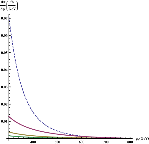
Figure 2: The same as in Fig. 1, but for larger values of $p_{\perp}$.

The differential cross sections at 13 TeV are shown in Figs. 3 and 4. Note that the gravity mediated contributions to the cross sections do not include the SM contribution (i.e. solid lines in all figures correspond to pure gravity contributions).

The figures for dimuon cross sections look similar to Figs. 1-4.

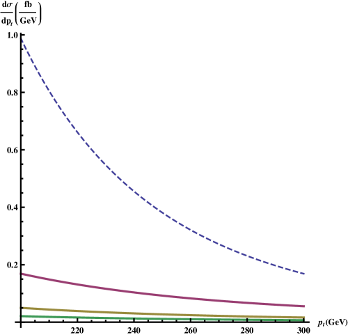
Figure 3: The KK graviton contribution to the dielectron production for $\bar{M}_{5}=4,6,8$ TeV (solid curves, from above) vs. SM (Born) contribution (dashed curve) at $\sqrt{s}=13$ TeV.

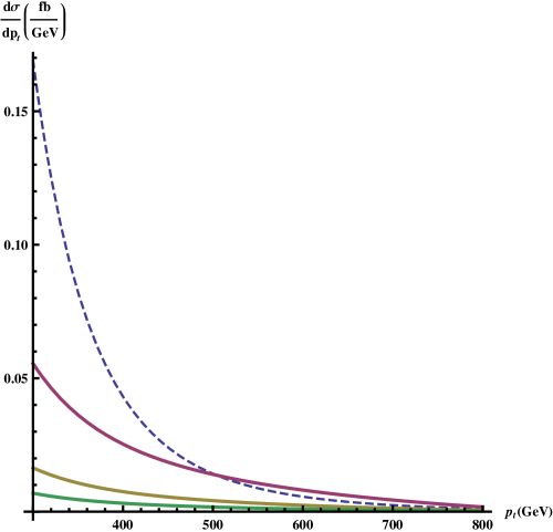
Figure 4: The same as in Fig. 3, but for larger values of $p_{\perp}$.

Let $N_{S}$($N_{B}$) be a number of signal (background) dilepton events with $p_{\perp}>p_{\perp}^{\mathrm{cut}}$,

$$N_{S}=\!\!\int\limits_{p_{\perp}>p_{\perp}^{\mathrm{cut}}}\!\!\frac{d\sigma(\mathrm{grav})}{dp_{\perp}}\,dp_{\perp}\;,\quad N_{B}=\!\!\int\limits_{p_{\perp}>p_{\perp}^{\mathrm{cut}}}\!\!\frac{d\sigma(\mathrm{SM})}{dp_{\perp}}\,dp_{\perp}\;.$$ (70)

Then we define the statistical significance $\mathcal{S}=N_{S}/\sqrt{N_{B}+N_{S}}$, and require a $5\sigma$ effect. In Fig. 5 the statistical significance is shown for total number of “events” with $\sqrt{s}=7$ TeV and $\sqrt{s}=8$ TeV as a function of the transverse momentum cut $p_{\perp}^{\mathrm{cut}}$ and reduced 5-dimensional gravity scale $\bar{M}_{5}$. The integrated luminosity was taken to be 5 fb^-1 and 20 fb^-1 for $\sqrt{s}=7$ TeV and $\sqrt{s}=8$ TeV, respectively.

Figure 5: The statistical significance $S$ for the dilepton ($\mathrm{\mu+e}$ ) production at the LHC for $\sqrt{s}=(7+8)$ TeV and integrated luminosity (5+20) fb^-1 as a function of the transverse momentum cut $p_{\perp}^{\mathrm{cut}}$ and reduced 5-dimensional gravity scale $\bar{M}_{5}$. The plane $\mathcal{S}=5$ is also shown.

Figure 6 represents the significance $\mathcal{S}$ for the dilepton events with $\sqrt{s}=13$ TeV and 30 fb^-1.

Figure 6: The same as in figure 5, but for $\sqrt{s}=13$ TeV and integrated luminosity 30 fb^-1.

Previously, calculations of dilepton cross sections were done in [3] without taking into account finite widths of the KK gravitons. As was shown in [1] (see also [12]), in zero width approximation the gravity cross sections are very small in comparison with the background cross section at low and moderate values of $p_{\perp}$. That is why, a high cut $p_{\perp}^{\mathrm{cut}}$ is needed in order to get $N_{S}$ comparable with $N_{B}$. Correspondingly, LHC search limits have appeared to be significantly smaller than in our case.

3 Conclusions

In the present paper the RSSC model [4]-[5] is considered in detail in which the reduced 5-dimensional Planck scale $\bar{M}_{5}$ can vary from few TeV to tens TeV, while the curvature $\kappa$ is allowed to vary from hundred MeV to few GeV. In fact, the only condition $\kappa\ll\bar{M}_{5}$ should be satisfied. The mass spectrum and experimental signature of the model with the small curvature are similar to those in the ADD model [9] with one flat extra dimension.

The $p_{\perp}$-distributions for the lepton pairs with high $p_{\perp}$ at the LHC are calculated for the collision energies 7, 8, and 13 TeV (for the dielectron case, the results of our calculations are shown in Figs. 1-2 and Figs. 3-4).

The account of the KK graviton widths is the crucial point for the numerical calculations, since the zero width approximation significantly underestimates the gravity cross sections even at large $p_{\perp}$.

The statistical significance as a function of the reduced 5-dimensional Planck scale $\bar{M}_{5}$ and cut on the lepton transverse momentum $p_{\perp}^{\mathrm{cut}}$ is calculated (see Figs. 5-6). Let us underline that both the dielectron and dimuon events are taken into account.

Recently, a search for large extra spatial dimensions in the dimuon (dielectron) channel was presented using a data sample of 20.6 fb^-1 (19.6 fb^-1) at the center-of-mass energy of 8 TeV collected by the CMS detector [16]-[17]. No significant deviations from SM were observed. Previously, dilepton spectra were found to be consistent with SM expectations at the energy of 7 TeV [18].

By using our calculations for 7 and 8 TeV, we conclude that in the RSSC framework the region

$$M_{5}<6.84\mathrm{\ TeV}$$ (71)

is excluded at 95$\%$ C.L. Note that for the ADD scenario the exclusion limits on the model parameter $M_{S}$ are 4.49 and 4.77 TeV for the dimuon and dielectron events, respectively [16]-[17].

Correspondingly, we obtain the discovery limit for the 13 TeV LHC with the integrated luminosity 30 fb^-1:

$$M_{5}=10.16\mathrm{\ TeV}\;.$$ (72)

In deriving Eqs. (71), (72), we used the relation $M_{5}=(2\pi)^{1/3}\bar{M}_{5}$ (6) in order to present the bounds on fundamental gravity scale $M_{5}$.

It is important that these bounds on $M_{5}$ do not depend on the curvature $\kappa$ (up to small powerlike corrections), contrary to the original RS1 model [2] in which estimated bounds on $M_{5}$ depend on the ratio $\kappa/\bar{M}_{\mathrm{Pl}}$.

Previously, analogous bounds were obtained for the diphoton production [12]. Recently, the LHC search limits were estimated for dimuon events [1]. Dilepton production at very high luminosities (HL-LHC) was studied in [19].

A Warped metric of RSSC model

From the action (1), 5-dimensional Einstein-Hilbert’s equations follow

$$\sqrt{|G|} \left(\mathcal{R}_{MN}-\frac{1}{2}\,G_{MN}\mathcal{R}\right)=-\frac{1}{2}\Big{[}\sqrt{|G|}\,G_{MN}\Lambda$$

$$+\sqrt{|g^{(1)}|}\,g^{(1)}_{\mu\nu}\,\delta_{M}^{\mu}\,\delta_{N}^{\nu}\,\delta(y)\,\Lambda_{1}+\sqrt{|g^{(2)}|}\,g^{(2)}_{\mu\nu}\,\delta_{M}^{\mu}\,\delta_{N}^{\nu}\,\delta(y-\pi r_{c})\,\Lambda_{2}\Big{]}\;.$$ (A.1)

In order to solve them, let us assume that the background metric respects 4-dimensional Poincare invariance ($\mu=0,1,2,3$)

$$\quad ds^{2}=e^{-2\sigma(y)}\,\eta_{\mu\nu}\,dx^{\mu}\,dx^{\nu}-dy^{2}\;,$$ (A.2)

After orbifolding (see Section 1), the coordinate of the extra compact dimension varies within the limits $0\leqslant y\leqslant\pi r_{c}$.

Let us define

$$g_{\mu\nu}=e^{-2\sigma(y)}\,\eta_{\mu\nu}\;.$$ (A.3)

Then the 5-dimensional background metric tensor looks like

$$G_{M\!N}=\left(\begin{array}[]{cc}g_{\mu\nu}&0\\ 0&-1\\ \end{array}\right)\;.$$ (A.4)

Correspondingly,

$$G^{M\!N}=\left(\begin{array}[]{cc}g^{\mu\nu}&0\\ 0&-1\\ \end{array}\right)\;,$$ (A.5)

with

$$g^{\mu\nu}=e^{2\sigma(y)}\,\eta^{\mu\nu}\;.$$ (A.6)

Non-trivial elements of the Christoffel symbols of the second kind looks like (there is no summation in $\mu$)

$$\Gamma^{\mu}_{\mu 4} =\frac{1}{2}\,g^{\mu\mu}\,\frac{\partial g_{\mu\mu}}{\partial y}=-\sigma^{\prime}(y)\,\delta_{\mu}^{\mu}\;,$$

$$\Gamma^{4}_{\mu\mu} =\frac{1}{2}\,\frac{\partial g_{\mu\mu}}{\partial y}=-\sigma^{\prime}(y)\,g_{\mu\mu}\;.$$ (A.7)

As a result, non-zero elements of the curvature tensor $\mathcal{R}_{K\!M,N\!L}$ are the following ($\mu\neq\nu$)

$$\mathcal{R}_{\mu 4,4\mu} =\mathcal{R}_{4\mu,\mu 4}=-\mathcal{R}_{\mu 4,\mu 4}=-\mathcal{R}_{4\mu,4\mu}=[\sigma^{\prime 2}(y)-\sigma^{\prime\prime}(y)]\,g_{\mu\mu}\;,$$

$$\mathcal{R}_{\mu\nu,\nu\mu} =\mathcal{R}_{\nu\mu,\mu\nu}=-\mathcal{R}_{\mu\nu,\mu\nu}=-\mathcal{R}_{\nu\mu,\nu\mu}=-\sigma^{\prime 2}(y)\,g_{\mu\mu}\,g_{\nu\nu}\;.$$ (A.8)

The non-zero elements of the Ricci tensor $\mathcal{R}_{M\!N}=G^{K\!L}\,\mathcal{R}_{K\!M,N\!L}$ are

$$\mathcal{R}_{44} =4[\sigma^{\prime 2}(y)-\sigma^{\prime\prime}(y)]\;,$$

$$\mathcal{R}_{\mu\mu} =[-4\sigma^{\prime 2}(y)+\sigma^{\prime\prime}(y)]\,g_{\mu\mu}\;.$$ (A.9)

The 5-dimensional scalar curvature $\mathcal{R}_{5}=G^{M\!N}\,\mathcal{R}_{M\!N}$ is equal to

$$\mathcal{R}_{5}=-20\sigma^{\prime 2}(y)+8\sigma^{\prime\prime}(y)\;.$$ (A.10)

Then the Einstein-Hilbert’s equations are reduced to

$$\sigma^{\prime 2}(y) =-\frac{\Lambda}{12}\;,$$ (A.11)

$$\sigma^{\prime\prime}(y) =\frac{1}{6}\,[\Lambda_{1}\,\delta(y)+\Lambda_{2}\,\delta(\pi r_{c}-y)]\;.$$ (A.12)

The first solution of this set of equations was presented in Ref. [2]

$$\sigma_{\mathrm{RS}}(y)=\kappa\,|y|\;,$$ (A.13)

with the cosmological constant

$$\Lambda_{\mathrm{RS}}=-12\kappa^{2}\;,$$ (A.14)

and boundary cosmological terms

$$\Lambda_{1}^{\mathrm{RS}}=-\Lambda_{2}^{\mathrm{RS}}=12\kappa\;.$$ (A.15)

Here $\kappa$ is a scale with the dimension of mass.

However, we get from (A.13) that $\sigma^{\prime\prime}_{\mathrm{RS}}(y)=2\kappa\,\delta(y)$ instead of $\sigma^{\prime\prime}(y)=\kappa[\delta(y)-\delta(\pi r_{c}-y)]$. Moreover, Eqs. (A.11), (A.12) say us that the cosmological constant $\Lambda$ should depend on coordinate $y$.

In the bulk the set of equations looks like

$$\sigma^{\prime 2}(y) =-\frac{\Lambda}{12}$$ (A.16)

$$\sigma^{\prime\prime}(y) =0\;,$$ (A.17)

with the evident solution

$$\sigma(y)=\kappa y+\mathrm{constant}\;,\quad\Lambda=-12\kappa^{2}\;.$$ (A.18)

Then we have for the full interval $0\leqslant y\leqslant\pi r_{c}$

$$\sigma^{\prime 2}(y) =\kappa^{2}z(y)\;,$$ (A.19)

$$\sigma^{\prime\prime}(y) =\frac{1}{6}\,[\Lambda_{1}\,\delta(y)+\Lambda_{2}\,\delta(\pi r_{c}-y)]\;,$$ (A.20)

where $z(y)=1$ for $0<y<\pi r_{c}$.

One obtains from Eq. (A.20)

$$\sigma^{\prime}(y)=\frac{1}{12}\,[\Lambda_{1}\,\tilde{\varepsilon}(y)+\Lambda_{2}\,\tilde{\varepsilon}(y-\pi r_{c})]+A\;,$$ (A.21)

where $A$ is a constant, and

$$\tilde{\varepsilon}(x)=\left\{\begin{array}[]{cc}d|x|/dx\;,&|x|>0\\ 1\;,&x=0\end{array}\right.$$ (A.22)

In fact, $\tilde{\varepsilon}(x)$ is the function $\varepsilon(x)=\theta(x)-\theta(-x)$ supplemented by its value at $x=0$. Let us note that $[\tilde{\varepsilon}(x)]^{2}=1$ for all $x$, and

$$\frac{1}{2}\,\left[\tilde{\varepsilon}(y)+\tilde{\varepsilon}(\pi r_{c}-y)\right]=\left\{\begin{array}[]{ll}0\;,&y<0\;,\\ 1\;,&0\leqslant y\leqslant\pi r_{c}\;,\\ 0\;,&y>\pi r_{c}\;.\end{array}\right.$$ (A.23)

Since the choice of $A$ is equivalent to a redefinition of $\Lambda_{1}$ and $\Lambda_{2}$, in what follows, we can put $A=0$.

As for the boundary cosmological terms $\Lambda_{1,2}$ and function $z(y)$, we get from (A.19) the equation

$$z(y)=\frac{1}{(12\kappa)^{2}}\,[\Lambda_{1}^{2}+\Lambda_{2}^{2}-2\Lambda_{1}\Lambda_{2}\,\tilde{\varepsilon}(y)\,\tilde{\varepsilon}(\pi r_{c}-y)]\;.$$ (A.24)

Thus, we obtain

$$\Lambda =-6\kappa^{2}[\tilde{\varepsilon}(y)+\tilde{\varepsilon}(\pi r_{c}-y)]\;,$$ (A.25)

$$\Lambda_{1} =-\Lambda_{2}=6\kappa\;.$$ (A.26)

As one can see from Eqs. (A.25) and (A.23), the cosmological constant $\Lambda$ is equal to $(-12\kappa^{2})$ at $0\leqslant y\leqslant\pi r_{c}$, and it is zero outside this region.

Finally, we find

$$\sigma(y)=\frac{\kappa}{2}\,(|y|-|\pi r_{c}-y|)+B\;,$$ (A.27)

where $B$ is a constant. Note that Eqs. (A.25), (A.26) differ from RS1 fine tuning solutions (A.14), (A.15).

To get the RSSC scenario, we take

$$B=-\frac{1}{2}\,\pi\kappa\,r_{c}\;.$$ (A.28)

Then

$$\sigma(y)=\frac{\kappa}{2}\,(|y|-|\pi r_{c}-y|-\pi r_{c})\;,$$ (A.29)

and we come to the metric (17).

The function $\sigma(y)$ (A.29) is $Z_{2}$–symmetric due to the periodicity condition (points $y-\pi r_{c}$ and $y+\pi r_{c}$ are identified). The $y$-dependent part of $\sigma(y)$ is symmetric under substitutions

$$y\rightarrow\pi r_{c}-y\;,\quad\kappa\rightarrow-\kappa\;.$$ (A.30)

It means that the branes are interchanged if we take an opposite sign for $\kappa$ (see comments to Eqs. (10)-(14) in the main text).

Note that the the Ricci tensor (A.10) is proportional to the metric tensor only in between the branes,

$$\mathcal{R}_{M\!N}=-4\kappa^{2}G_{M\!N}=\frac{\Lambda}{3}\,G_{M\!N}\;,\quad 0<y<\pi r_{c}\;,$$ (A.31)

with $\Lambda$ being cosmological constant. For a space-time with the constant curvature $K$, the following equation holds

$$R_{K\!M,N\!L}=K\left(G_{K\!N}\,G_{M\!L}-G_{K\!L}\,G_{M\!N}\right)\;,$$ (A.32)

and we find

$$K=\kappa^{2}\;.$$ (A.33)

Correspondingly, the radius of the curvature in the bulk is

$$\rho=\frac{1}{\kappa}\;.$$ (A.34)

At the boundaries, both the tensors $\mathcal{R}_{K\!M,N\!L}$, $\mathcal{R}_{M\!N}$ and scalar curvature $\mathcal{R}_{5}$ have singular terms, as one can see from Eqs. (A Warped metric of RSSC model)-(A.10) and (A.20).

B Normalization of graviton wave functions

The normalization constants are obtained from the following relation ($n>0$)

$$1=\frac{1}{\pi r_{c}}\int_{0}^{\pi r_{c}}\!\!dy\,e^{-2\sigma(y)}[\psi^{(n)}(z_{n})]^{2}=\frac{1}{\pi\kappa r_{c}b_{n}^{2}}\,N_{n}^{2}\,I_{n}\;,$$ (B.1)

where

$$I_{n}=\int_{a_{n}}^{b_{n}}\!\!dzz\left[J_{2}(z)Y_{1}(b_{n})-Y_{2}(z)J_{1}(b_{n})\right]^{2}\;.$$ (B.2)

The parameters $a_{n}$ and $b_{n}$ are defined in the main text (see Eqs. (38), (36)).

To calculate $I_{n}$, we use the table integral [20],

$$\int^{x}\!\!\!dzZ_{\nu}(z)Z^{\,\prime}_{\nu}(z)=\frac{x^{2}}{4}\big{[} 2Z_{\nu}(x)Z^{\,\prime}_{\nu}(x)-Z_{\nu+1}(x)Z^{\,\prime}_{\nu-1}(x)$$

$$-Z_{\nu-1}(x)Z^{\,\prime}_{\nu+1}(x)\big{]}+\mathrm{constant}\;,$$ (B.3)

where $Z_{\nu},\,Z^{\,\prime}_{\nu}=J_{\nu}$ or $Y_{\nu}$, as well as relations between Bessel functions,

$$J_{\nu+1}(x)Y_{\nu}(x)-Y_{\nu+1}(x)J_{\nu}(x) =\frac{2}{\pi x}\;,$$

$$J_{\nu+2}(x)Y_{\nu}(x)-Y_{\nu+2}(x)J_{\nu}(x) =\frac{4(\nu+1)}{\pi x^{2}}\;.$$ (B.4)

Then the integral (B.2) is equal to

$$I_{n} =2a_{n}[J_{1}(a_{n})Y_{1}(b_{n})-Y_{1}(a_{n})J_{1}(b_{n})][J_{2}(a_{n})Y_{1}(b_{n})-Y_{2}(a_{n})J_{1}(b_{n})]\;,$$

$$-\frac{a_{n}^{2}}{2}[J_{1}(a_{n})Y_{1}(b_{n})-Y_{1}(a_{n})J_{1}(b_{n})]^{2}$$

$$-\frac{a_{n}^{2}}{2}[J_{2}(a_{n})Y_{1}(b_{n})-Y_{2}(a_{n})J_{1}(b_{n})]^{2}+\frac{2}{\pi^{2}}\;.$$ (B.5)

Due to the left boundary condition in the form (37), two first terms in the r.h.s of Eq. (B Normalization of graviton wave functions) vanish, and we get

$$I_{n}=\frac{2}{\pi^{2}}\left[1-\frac{Y_{1}^{2}(b_{n})}{Y_{1}^{2}(a_{n})}\right]=\frac{2}{\pi^{2}}\left[1-\frac{J_{1}^{2}(b_{n})}{J_{1}^{2}(a_{n})}\right]\;.$$ (B.6)

As a result, we find the expression for the normalization constant

$$N_{n}^{-2}=\frac{2}{\kappa r_{c}\pi^{3}b_{n}^{2}}\left[\frac{Y_{1}^{2}(a_{n})-Y_{1}^{2}(b_{n})}{Y_{1}^{2}(a_{n})}\right]\;.$$ (B.7)

Our formula (B.7) is in agreement with that from Ref. [3].

For $n\neq m$, we have

$$\int_{0}^{\pi r_{c}}\!\!\!dy\,e^{-2\sigma(y)}\,\psi^{(n)}(y)\,\psi^{(m)}(y)=\frac{1}{\kappa}\,N_{n}N_{m}\,I_{nm}\;,$$ (B.8)

where

$$I_{nm}=\int_{e^{-\pi\kappa r_{c}}}^{1}\!\!\!dzz\, [J_{2}(b_{n}z)Y_{1}(b_{n})-Y_{2}(b_{n}z)J_{1}(b_{n})]$$

$$\times [J_{2}(b_{m}z)Y_{1}(b_{m})-Y_{2}(b_{m}z)J_{1}(b_{m})]\;.$$ (B.9)

By using table integral [20],

$$\int^{x}\!\!\!dzzZ_{\nu}(az)Z^{\,\prime}_{\nu}(bz) =\frac{x}{a^{2}-b^{2}}[aZ_{\nu+1}(ax)Z^{\,\prime}_{\nu}(bx)-bZ_{\nu}(ax)Z^{\,\prime}_{\nu+1}(bx)]$$

$$+\mathrm{constant}\;,$$ (B.10)

and Eq. (37), one can be easily show that $I_{nm}=0$.

C Cross section for dilepton production

The differential cross section of the DY process (63) is given by ($l=e$ or $\mu$)

$$\frac{d\sigma}{dp_{\perp}}(pp\rightarrow l^{+}l^{-}+X) =2p_{\perp}\!\!\!\!\sum\limits_{a,b=q,\bar{q},g}\!\!\int\nolimits\!\!\frac{d\tau\sqrt{\tau}}{\sqrt{\tau-x_{\perp}^{2}}}\!\int\nolimits\!\frac{dx_{1}}{x_{1}}f_{a/p}(\mu^{2},x_{1})$$

$$\times f_{b/p}(\mu^{2},\tau/x_{1})\,\frac{d\sigma}{d\hat{t}}(ab\rightarrow l^{+}l^{-})\;,$$ (C.1)

with the transverse energy of the lepton pair equals to $2p_{\perp}$. In (C Cross section for dilepton production) two dimensionless quantities are introduced

$$x_{\perp}=\frac{2p_{\perp}}{\sqrt{s}}\;,\quad\tau=x_{1}x_{2}\,,$$ (C.2)

where $x_{2}$ is the momentum fraction of the parton $b$ in (C Cross section for dilepton production).

Without cuts, integration variables in (C Cross section for dilepton production) vary within the following limits

$$x_{\perp}^{2}\leq\tau\leq 1\;,\quad\tau\leq x_{1}\leq 1\;.$$ (C.3)

After imposing kinematical cut on lepton rapidity, the integration region becomes more complicated (see Appendix A in Ref. [1]).

The SM contribution to the $p_{\perp}$-distribution looks like

$$\frac{d\sigma^{\mathrm{SM}}}{d\hat{t}}(q\bar{q}\rightarrow l^{+}l^{-})=\frac{1}{48\pi s^{2}}\left[u^{2}\left(|G^{LL}|^{2}+|G^{RR}|^{2}\right)+t^{2}\left(|G^{LR}|^{2}+|G^{RL}|^{2}\right)\right]\;,$$ (C.4)

with

$$G^{AB}(s)=\sum_{V=\gamma,Z}\!\frac{g_{A}(V\rightarrow l^{+}l^{-})\,g_{A}(V\rightarrow q\bar{q})}{s-m_{V}^{2}+im_{V}\Gamma_{V}}\;.$$ (C.5)

Here $g_{L(R)}(\gamma\rightarrow l^{+}l^{-})=g_{L(R)}(\gamma\rightarrow q\bar{q})=e$, and

$$g_{L}(Z\rightarrow l^{+}l^{-}) =-\frac{1}{2}+\sin^{2}\theta_{W}\;,$$

$$g_{R}(Z\rightarrow l^{+}l^{-}) =\ \sin^{2}\theta_{W}\;,$$

$$g_{L}(Z\rightarrow q\bar{q}) =T_{3}^{q}-e_{q}\sin^{2}\theta_{W}\;,$$

$$g_{R}(Z\rightarrow q\bar{q}) =-e_{q}\sin^{2}\theta_{W}\;,$$ (C.6)

with $T_{3}^{q}$ being third component of the quark isospin, $e_{q}$ being quark electric charge (in units of $|e|$).

The graviton contribution comes from both quark-antiquark annihilation and gluon-gluon fusion subprocesses (see, for instance, [3])

$$\frac{d\sigma^{\mathrm{grav}}}{d\hat{t}}(q\bar{q}\rightarrow l^{+}l^{-}) = \frac{\hat{s}^{4}+10\hat{s}^{3}\hat{t}+42\,\hat{s}^{2}\hat{t}^{2}+64\hat{s}\,\hat{t}^{3}+32\,\hat{t}^{4}}{1536\,\pi\hat{s}^{2}}\left|\mathcal{S}(\hat{s})\right|^{2}\;,$$

$$\frac{d\sigma^{\mathrm{grav}}}{d\hat{t}}(gg\rightarrow l^{+}l^{-}) = -\frac{\hat{t}(\hat{s}+\hat{t})(\hat{s}^{2}+2\hat{s}\,\hat{t}+2\,\hat{t}^{2})}{256\,\pi\hat{s}^{2}}\left|\mathcal{S}(\hat{s})\right|^{2}\;,$$ (C.7)

where

$$\mathcal{S}(s)=\frac{1}{\Lambda_{\pi}^{2}}\sum_{n=1}^{\infty}\frac{1}{s-m_{n}^{2}+i\,m_{n}\Gamma_{n}}\;$$ (C.8)

is the invariant part of the partonic matrix elements, with $\Gamma_{n}$ being total width of the graviton with the KK number $n$ and mass $m_{n}$ [5]:

$$\Gamma_{n}=\eta\,m_{n}\left(\frac{m_{n}}{\Lambda_{\pi}}\right)^{2},\quad\eta\simeq 0.09\;.$$ (C.9)

Let us note that the function $\mathcal{S}(s)$ is the same for all processes mediated by $s$-channel virtual gravitons.

In the RSSC model, an explicit form for the sum (C.8) was obtained for $\bar{M}_{5}\gg\kappa$ in Ref. [5]

$$\mathcal{S}(s)=-\frac{1}{4\bar{M}_{5}^{3}\sqrt{s}}\;\frac{\sin 2A+i\sinh 2\varepsilon}{\cos^{2}\!A+\sinh^{2}\!\varepsilon}\;,$$ (C.10)

where

$$A=\frac{\sqrt{s}}{\kappa}\;,\qquad\varepsilon=\frac{\eta}{2}\Big{(}\frac{\sqrt{s}}{\bar{M}_{5}}\Big{)}^{3}\;.$$ (C.11)

It is important to underline that the magnitude of $\mathcal{S}(s)$ is defined by the fundamental gravity scale $\bar{M}_{5}$, not by the scale $\Lambda_{\pi}$ presented in the Lagrangian. In general, this property is valid in the RSSC model for both real and virtual production of the KK gravitons [4, 5].

References

• [1] A.V.ย Kisselev, JHEP 04 (2013) 025 [arXiv:1210.3238].
• [2] L.ย Randall and R.ย Sundrum, Phys. Rev. Lett. 83 (1999) 3370 [hep-ph/9905221].
• [3] G.ย F.ย Giudice, T.ย Plehn and A.ย Strumia, Nucl. Phys. B 706 (2005) 455 [hep-ph/0408320].
• [4] A.V.ย Kisselev and V.A.ย Petrov, Phys. Rev. D 71 (2005) 124032 [hep-ph/0504203].
• [5] A.V.ย Kisselev, Phys. Rev. D 73 (2006) 024007 [hep-th/0507145].
• [6] H. Davoudiasl, J.L. Hewett and T.G. Rizzo, Phys. Rev. Lett. 84 (2000) 2080 [hep-ph/9909255].
• [7] M.ย Toharia, Mod. Phys. Lett. A 19 (2004) 37 [arXiv:0212036].
• [8] E.E.ย Boos, Yu.A.ย Kubyshin, M.N.ย Smolyakov and I.P.ย Volobuev, Class. Quant. Grav. 19 (2002) 4591 [hep-th/0202009].
• [9] N.ย Arkani-Hamed, S.ย Dimopoulos and G.ย Dvali, Phys. Lett. B 429 (1998) 263 [hep-ph/9803315].
• [10] I.ย Antoniadis, N.ย Arkani-Hamed, S.ย Dimopoulos and G.ย Dvali, Phys. Lett. B 436 (1998) 257 [hep-ph/9804398].
• [11] N.ย Arkani-Hamed, S.ย Dimopoulos and G.ย Dvali, Phys. Rev. D 59 (1999) 086004 [hep-ph/9807344].
• [12] A.V.ย Kisselev, JHEP 09 (2008) 039 [arXiv:0804.3941].
• [13] V.A.ย Rubakov, Phys. Usp. 44 (2001) 871 [hep-ph/0104152].
• [14] CMS collaboration, Phys. Lett. B 711 (2012) 15 [arXiv:1202.3827].
• [15] A.ย Martin, W.ย Stirling, R.ย Thorne and G.ย Watt,Eur. Phys. J. C 63 (2009) 189 [arXiv:0901.0002].
• [16] CMS Collaboration, CMS-PAS-EXO-12-027.
• [17] CMS Collaboration, CMS-PAS-EXO-12-031.
• [18] CMS Collaboration, Phys. Lett. B 711 (2012) 15 [arXiv:1202.3827].
• [19] A.V. Kisselev, RS model with a small curvature and Drell-Yan process at the LHC, in Proceedings of CMS Workshop on Perspectives on Physics and on CMS at Very High Luminosity, Alushta, Ukraine, 2012. Dubna: JINR, E1-2013-96, p.ย 155 [arXiv:1208.3844].
• [20] A.P.ย Prudnikov, Yu.A.ย Brychkov and O.I.ย Marichev, Integrals and Series, Vol.ย 2: Special Functions, Gordon and Breach Sci. Publ., N.Y. (1986).