Dynamic Partitioning-based JPEG Decompression on Heterogeneous Multicore Architectures

Abstract

With the emergence of social networks and improvements in computational photography, billions of JPEG images are shared and viewed on a daily basis. Desktops, tablets and smartphones constitute the vast majority of hardware platforms used for displaying JPEG images. Despite the fact that these platforms are heterogeneous multicores, no approach exists yet that is capable of joining forces of a system’s CPU and GPU for JPEG decoding.

In this paper we introduce a novel JPEG decoding scheme for heterogeneous architectures consisting of a CPU and an OpenCL-programmable GPU. We employ an offline profiling step to determine the performance of a system’s CPU and GPU with respect to JPEG decoding. For a given JPEG image, our performance model uses (1) the CPU and GPU performance characteristics, (2) the image entropy and (3) the width and height of the image to balance the JPEG decoding workload on the underlying hardware. Our run-time partitioning and scheduling scheme exploits task, data and pipeline parallelism by scheduling the non-parallelizable entropy decoding task on the CPU, whereas inverse cosine transformations (IDCTs), color conversions and upsampling are conducted on both the CPU and the GPU. Our kernels have been optimized for GPU memory hierarchies.

We have implemented the proposed method in the context of the libjpeg-turbo library, which is an industrial-strength JPEG encoding and decoding engine. Libjpeg-turbo’s hand-optimized SIMD routines for ARM and x86 constitute a competitive yardstick for the comparison to the proposed approach. Retro-fitting our method with libjpeg-turbo provides insights on the software-engineering aspects of re-engineering legacy code for heterogeneous multicores.

We have evaluated our approach for a total of 7194 JPEG images across three high- and middle-end CPU–GPU combinations. We achieve speedups of up to 4.2x over the SIMD-version of libjpeg-turbo, and speedups of up to 8.5x over its sequential code. Taking into account the non-parallelizable JPEG entropy decoding part, our approach achieves up to 95% of the theoretically attainable maximal speedup, with an average of 88%.

erformance, Algorithms, Design

1 Introduction

The JPEG format is the de facto compression standard for digital images in a wide range of fields from medical imaging to personal digital cameras. By our own observation, 463 out of the 500 most popular websites Alexa Top 500 Global Sites [retrieved Feb. 2013] use JPEG images (including Google, Facebook, Youtube and Baidu). With the emergence of social networks and innovations in computational photography, billions of JPEG images are shared and viewed on a daily basis: Facebook reported in 2010 already to store over 65 billion photos Beaver et al. [2010], and the Instagram photo-sharing service claims to have 45 million daily uploads Instagram Press Center [retrieved Jun. 2013]. Similar numbers can be assumed for other photo hosting and sharing services such as Flickr and Photobucket.

Desktops, tablets and smartphones constitute the vast majority of hardware platforms used for viewing JPEG images. Although these platforms are nowadays equipped with a CPU and GPU, to the best of our knowledge no approach is available yet that is capable of incorporating both the CPU and the GPU for JPEG decoding.

Libjpeg Libjpeg [retrieved Jun. 2013] is a sequential JPEG reference implementation by the Independent JPEG Group. To accelerate image processing, the libjpeg-turbo Libjpeg Turbo [retrieved Jun. 2013] re-implementation applies SIMD instructions with a single thread of execution on x86 and ARM platforms. We have observed that the SIMD-version of libjpeg-turbo decodes an image twice as fast as the sequential version on an Intel i7. Libjpeg-turbo is widely used, e.g., with the Google Chrome and Firefox web-browsers, WebKit The WebKit Open Source Project [retrieved Jun. 2013], and the Ubuntu, Fedora and openSUSE Linux distributions. Neither libjpeg nor libjpeg-turbo are capable of utilizing a GPU.

JPEG decoding is computationally expensive, consisting of Huffman decompression, dequantization, IDCT, image upsampling and YCbCr to RGB color space conversion. Among all stages, Huffman decompression is strictly sequential, because code-words have variable lengths and the start of a codeword in the encoded bitstream is only known once the previous codeword has been decoded. A sub-class of Huffman codes that provide the so-called self-synchronization property Capocelli et al. [1988] are suitable for decoding multiple chunks of the encoded bitstream in parallel, as proposed in Klein and Wiseman [2003]. However, the JPEG standard does not enforce the self-synchronization property Wallace [1991]. In our implementation, Huffman decoding is therefore executed sequentially on the CPU. The remaining stages have repetitive computations and low data dependencies, which makes them suitable to exploit data, task and pipeline-parallelism.

A desktop GPU has several hundreds of scalar processors, offering more parallelism than what is provided by nowaday’s SIMD CPU instruction set architectures. GPUs offer a higher memory bandwidth than CPUs. However, a GPU core lacks complex control units and operates at a much lower clock frequency. The PCI bus that connects the GPU to the CPU represents a bandwidth-bottleneck that incurs significant overhead to computations on the GPU. JPEG decoding on a GPU is thus not necessity faster than the SIMD-version of libjpeg-turbo on a CPU. Nevertheless, utilizing both CPU and GPU has the potential to achieve the highest overall performance, regardless of the computational power of the CPU and GPU.

Consequently, this paper makes the following contributions:

• we propose a performance model based on off-line profiling that characterizes all JPEG decoding steps for a given CPU-GPU combination from multivariate polynomial regression. We identified image entropy and the image dimensions as the only required parameters for our performance model,

• we propose a dynamic partitioning scheme that automatically distributes the workload across CPU and GPU at run-time according to our performance model,

• we optimize JPEG decoding on GPUs by employing data vectorization, intermediate local memory and coalesced memory accesses,

• we boost parallelism by utilizing a pipelined execution model that overlaps sequential Huffman decoding with GPU computations,

• we report on the software engineering aspects of refactoring the libjpeg-turbo legacy code for heterogeneous multicores, and

• we present experimental results on three representative high- and mid-end CPU-GPU architectures for the applicability and efficiency of our approach. We achieve speedups up to 4.2x over the SIMD-version of libjpeg-turbo, and up to 8.5x over its sequential code. We achieve up to 95% of the theoretically attainable speedup, with 88% on average.

The remainder of this paper is organized as follows: Section 2 presents background information on JPEG decoding; libjpeg-turbo re-engineering is discussed in Section 3. Our OpenCL JPEG decoding kernels for GPUs are presented in Section 4. Section 5 describes the performance model and dynamic partitioning scheme for a system consisting of a CPU and a GPU. Section 6 contains the experiential results. We discuss the related work in Section 7 and draw our conclusions in Section 8.

2 Background: JPEG Decoding

Figure 1 describes the decoding steps to produce an uncompressed bitmap from a JPEG image. A JPEG file is structured as a sequence of segments, including image dimensions, component subsampling, Huffman and quantization tables and entropy-coded data. Entropy-coded data is the largest part of a JPEG file, and thus, has the highest contribution to the file size. Color in JPEG-encoded images is represented by luminance (Y), blue chrominance (Cb) and red chrominance (Cr) component values. Because the human eye is more sensitive to changes in luminance than changes in chrominance, the spatial resolution of chrominance components are commonly compressed. This process is called downsampling. In 4:2:2 subsampling, the Y component is sampled at each pixel while Cb and Cr components are sampled every two pixels in horizontal direction. 4:4:4 sampling has the same sample rate across all components and downsampling is not required Poynton [Retrieved July 2013].

Figure 1: JPEG decoder path.

An image is divided into blocks of 8x8 pixels. JPEG decompression operates in units of minimum coded units (MCUs), which are minimum sets of blocks from each color component. The MCU size for 4:4:4 subsampling is 8x8 pixels in libjpeg-turbo. In 4:2:2 subsampling, one chrominance block is upsampled to two blocks horizontally. Thus, an MCU has a size of 16x8 pixels. The decoder first decodes entropy data, then de-quantizes it according to an image-specific quantization table. IDCT transforms MCUs from the frequency domain back to the spatial domain. The libjpeg and libjpeg-turbo libraries apply a series of 1D IDCTs based on the AAN algorithm Yukihiro et al. [1988]; Pennebaker and Mitchell [1992]. If the image subsampling is not 4:4:4, it must be upsampled to restore the spatial resolution of chrominance components to the original size. Color conversion converts the Y, Cr and Cb samples of each pixel to the RGB color space. Apart from Huffman decoding, all JPEG decoding steps contain few data dependencies and a large amount of data-parallelism. In fact, libjpeg-turbo utilizes SIMD instructions for all stages except Huffman decoding.

3 Re-engineering the Libjpeg-turbo Software Architecture for Heterogeneous Multicores

Libjpeg-turbo has been designed with a consideration of memory resources. Both encoder and decoder operate in units of MCU rows. The software architecture of libjpeg-turbo is illustrated in Figure 2. The decoder uses a 2-tier controller and buffer hierarchy to control decoding and storage of a single MCU row in various stages.

Figure 2: Libjpeg-turbo software architecture.

We identified two shortcomings which hamper parallelizing the library for heterogeneous multicores. First, because decoding is done in units of MCU rows, additional, unnecessary dependencies between subsequent MCU rows are introduced. These dependencies limit the possible achievable parallelism in three ways:

1. A single MCU row of an image may not contain enough data to utilize a GPU. Most of the computationally intensive operations, i.e., IDCT, upsampling and color conversion, are data-parallel tasks where more data means more parallelism. Equally worse, pipeline-parallelism between decoding steps is impossible because of those dependencies.

2. Transferring row after row of image data from CPU to GPU is inefficient, because initiating a transfer induces constant overhead. Transferring a large amount of data in one transfer is thus more efficient than using several smaller transfers.

3. For each MCU row, a kernel invocation on the GPU is required.

Second, for modularity reasons, the libjpeg-turbo library has been designed in two major parts: coefficient control and postprocessing control. A 2-tier buffer hierarchy abstracts away the actual decoding work, and function pointers are used to encapsulate decoding functionality (e.g., integer vs. float IDCT). The segmented software architecture makes it very hard to re-use JPEG decoder components, because the buffer hierarchy permeates all components.

We re-engineered the libjpeg-turbo library under two objectives: (1) to be minimally invasive to the legacy code, and (2) to support massively parallel architectures. To prevent expensive CPU-GPU data transfers, we introduced an additional input and output buffer below the existing buffer hierarchy. These buffers are large enough to keep an image as a whole in memory. (Note that this fits in naturally with JPEG decoding, e.g., a web-browser will initiate decoding once the whole image or a large part of it is available in main memory.) The new whole-image buffers allowed us to transfer sufficiently large chunks of the image between CPU and GPU, while providing the legacy-code on the CPU with its “accustomed” row-by-row access, thereby keeping the changes to the existing library code to a minimum. The kernel codes for the GPU were implemented in OpenCL. The existing library code served as the starting point for the GPU code, with all GPU-specific optimizations explained in Section 4.

4 JPEG Decoding on the GPU

After entropy (Huffman) decoding, the CPU transfers a buffer of decoded data to the GPU. The IDCT, upsampling and color conversion kernels are invoked subsequently. Our chosen buffer layout has Y blocks followed by Cb blocks followed by Cr blocks. The upsampling kernel does not have to read the Y-space. This buffer layout avoids interleaving block access, and thus, improves coalesced memory access. At the end of color conversion, the output image in RGB color is transferred to a designated memory location of the whole-image output buffer (see Section 3) on the CPU.

4.1 Inverse Discrete Cosine Transformation (IDCT)

The entropy-decoded data in the frequency domain is transformed back to the spatial domain using a 2D IDCT. We implemented the 2D IDCT algorithm by applying a 1D IDCT to eight columns of a block (column pass) and then to eight rows of the result (row pass), as shown in Equation (1) and Equation (2) respectively.

$$f(u,y)=\sum_{v=0}^{N-1}C_{v}F(u,v)\cdot\cos\left(\frac{(2y+1)v\pi}{2N}\right),$$ (1)

$$f(x,y)=\sum_{u=0}^{N-1}C_{u}f(u,y)\cdot\cos\left(\frac{(2x+1)u\pi}{2N}\right),$$ (2)

where

$$0\leq x,y\leq N-1:\thinspace\text{spatial coordinates},$$

$$0\leq u,v\leq N-1:\thinspace\text{frequency coordinates},$$

$$C_{u},C_{v}=\frac{1}{\sqrt{2}}\text{ for }u,v=0,\text{ otherwise }1.$$

We employ eight OpenCL work-items per block. The input data is de-quantized after being loaded from global memory. Each work-item performs the column pass followed by the row pass. A work-item stores an eight-pixel column directly to its registers such that no communication is required among work-items. The intermediate results from the column pass are shared among work-items within a group to process the row pass. Thus, local memory is the suitable choice.

Each work-item holds eight elements of 8-bit color representation at the end of the row pass. Copying eight times would generate an excessive overhead. Hence, we vectorize the elements to reduce global memory access requests.

Instructions are issued per group of work-items called a warp in NVIDIA’s terminology. The warp size is typically 32. Therefore, a work-group performs IDCT on a multiple of four blocks to ensure that the number of work-items per group is a multiple of 32. The optimal work-group size is hardware-specific and is determined during profiling (see Section 5).

4.2 Upsampling

The chrominance color space with 4:2:2 subsampling is downsampled to half of the luminance space during JPEG encoding. The sample rates of these color spaces must be upsampled to the original size. Algorithm 1 describes an upsampling process that takes an 8-pixel row as an input to generate a 16-pixel row.

1 Out[0] = In[0]

2 Out[1] = (In[0] * 3 + In[1] + 2) / 4

3 Out[2] = (In[1] * 3 + In[0] + 1) / 4

4 Out[3] = (In[1] * 3 + In[2] + 2) / 4

5 Out[4] = (In[2] * 3 + In[1] + 1) / 4

6 Out[5] = (In[2] * 3 + In[3] + 2) / 4

7 Out[6] = (In[3] * 3 + In[2] + 1) / 4

8 Out[7] = (In[3] * 3 + In[4] + 2) / 4

9 Out[8] = (In[4] * 3 + In[3] + 1) / 4

10 Out[9] = (In[4] * 3 + In[5] + 2) / 4

11 Out[10] = (In[5] * 3 + In[4] + 1) / 4

12 Out[11] = (In[5] * 3 + In[6] + 2) / 4

13 Out[12] = (In[6] * 3 + In[5] + 1) / 4

14 Out[13] = (In[6] * 3 + In[7] + 2) / 4

15 Out[14] = (In[7] * 3 + In[6] + 1) / 4

Out[15] = In[7]

Algorithm 1 Upsampling for 4:2:2 subsampling.

We utilize 16 OpenCL work-items to perform upsampling on one block. Two work-items process one row of the block. The work-item with the even ID reads In[0] to In[4] to produce an eight-pixel row from Out[0] to Out[7], and the work-item with the odd ID reads In[4] to In[7] to produce the successive eight-pixel row Out[8] to Out[15].

The output equations have fixed patterns for odd indices and even indices. It should be noted that all but the end pixels depend on the neighbouring pixels of a block. The computations of Out[0] and Out[8] happen concurrently, and the same situation occurs with Out[7] and Out[15]. The computational pattern of the end pixels is different from the other pixels. Consequently, an if-statement is required to determine the correct equation for a specific work-item. An if-statement causes branch divergence if less than half of a warp take the same branch. We chose the work-group size such that 16 work-items take the same branch. This access pattern was designed to favour a merged upsampling-color conversion kernel, which is explained in Section 4.4.

4.3 Color Conversion

The final stage of the JPEG decoder converts the YCbCr color space to the RGB color space according to Algorithm 2. A work-item accesses global memory three times for its Y, Cb and Cr values to calculate R, G and B values for one pixel. The computations for each pixel are independent of other pixels.

Input : Pixel information in YCbCr color space

Output : Pixel information in RGB color space

1 R = Y + 1.402 (Cr - 128)

2 G = Y - 0.34414 (Cb - 128) - 0.71414 (Cr - 128)

B = Y + 1.772 (Cb - 128)

Algorithm 2 Cb/Cr to RGB color space conversion.

The buffers for IDCT and upsampling are arranged as a sequence of blocks, shown in Figure 3(a). However, the output buffer of color conversion is arranged as a sequence of pixels starting from the top-left pixel of the image then traverses row-wise to the bottom-right pixel of the image as shown in Figure 3(b). We devised an indexing function that calculates the index of the next pixel in vertical direction to be one image-width apart.

(a) Block-based pattern

(b) Pixel-based pattern

Figure 3: Buffer layouts of an 16x8 image 3(a) before color conversion and 3(b) after color conversion. The blue line indicates the access pattern.

The final output of the image is represented in interleaved RGB color space. Each R, G and B value is represented as an unsigned character. Similar to IDCT, vectorization in groups of four elements can be applied. In NVIDIA’s device compute capability 2.x or higher, global memory write instructions support 1, 2, 4, 8 or 16 bytes Nvidia Corporation [2012]. However, a pixel consists of three bytes. Therefore, a work-item should perform color conversion on a multiple of four pixels. An eight-pixel row has 24 elements. We group for pixels to six vectors of four elements as shown in Figure 4. The number of transfers is thereby reduced by a factor of four.

Figure 4: Vectorization of interleaving RGB performed by one work-item in order to reduce global memory writes.

4.4 GPU Kernel Merging

Previously stored data in local memory is no longer accessible on the next kernel invocation. Intermediate results must be stored back to global memory at the end of each kernel invocation, which generates unnecessary memory traffic. Because the computation of color conversion has no data dependency among pixels, it can be merged with the preceding kernel to reduce global memory accesses.

An image with 4:4:4 subsampling does not require upsampling. The color conversion kernel is merged with the IDCT kernel. Color conversion requires information from all color spaces. Therefore, the IDCT kernel repeats the computation three times for the three color spaces. At the end of IDCT, a work-item holds Y, Cb and Cr rows in its registers. The work-item immediately performs color conversion on the row without additional communication with other work-items. Although a single work-item now performs three times more IDCT computations, the storing of intermediate results in global memory between the IDCT and color conversion kernel invocations are avoided.

With 4:2:2 subsampling, the color conversion and upsampling kernels are combined. We use two OpenCL work-items to perform upsampling on a Cb and Cr row such that at the end of upsampling, chrominance information of one row is stored in the registers of each work-item. Only a row of Y space of the corresponding pixels is loaded from global memory before starting color conversion. Our work-group in the merged kernel, consisting of 128 work-items, processes two groups of four blocks. Sixteen work-items are allocated per block, and 64 work-items compute upsampling on the same index of different eight-pixel row segments to avoid branch-divergence. At the end of upsampling, this work-group produces sixteen image blocks.

We considered merging IDCT, upsampling and color conversion into one kernel. Nevertheless, combining all kernels is not favourable because the number of available registers constrains the number of active work-groups per multiprocessor.

4.5 Pipelined Kernel Execution

We observed that Huffman decoding consumed around half of the overall execution time with the SIMD-version of libjpeg-turbo. Huffman decoding is sequential and thus performed exclusively on the CPU. Subsequent decoding steps, i.e., IDCT, upsampling and color conversions are highly data-parallel and thus allocated to the GPU. In the following, we refer to those steps as the parallel part of JPEG decoding. In the execution model explained so far, GPU computations are delayed until decoded entropy data becomes available, as shown in Figure 5(a). Because the GPU is un-utilized during Huffman decoding, potential speedup is lost. Using the fact that entropy data is decoded in order, GPU computations can start after sufficient image rows have been decoded. Hence, Huffman decoding and GPU kernel execution can be executed in a pipelined fashion, where the first pipeline stage, i.e., Huffman decoding, is executed on the CPU, and the second pipeline stage, i.e., the parallel part, is executed on the GPU. Figure 5(b) shows the timeline of our pipelined execution mode.

An image is sliced horizontally into several chunks. As soon as the first chunk is entropy decoded, the CPU transfers the data to the GPU. All OpenCL commands are executed asynchronously. Hence, the CPU can resume Huffman decoding immediately for the second chunk. The execution time of the GPU kernel may not match the Huffman decoding time, because Huffman decoding varies greatly with the image details contained in a chunk. If the GPU is faster than the CPU, GPU computations are hidden behind Huffman-decoding on the CPU. The overall execution time then consists of the Huffman decoding time of the entire image plus the kernel invocation for the last portion of the image.

The most efficient chunk size is determined through static profiling on large images. Chunk sizes are varied from the full height down to an eight pixel stripe. The decoding speed tends to be faster as the number of chunks increases. However, as chunks become too small, GPU utilization becomes low. The best sizes from each image are selected. The final partition size is chosen as the largest size on the best list to prevent from choosing a size that is too small wrt. GPU utilization.

(a) Normal GPU execution

(b) Pipeline execution

Figure 5: JPEG decompression timelines: 5(a) GPU execution of the parallel part after Huffman decoding and 5(b) pipelined execution of Huffman decoding and GPU computations. The CPU reads back the results at the end of each kernel invocation. The read arrows have been omitted for clarity.

5 Heterogeneous JPEG Decoding

Low-end GPUs may be incapable of out-performing high-end CPUs. For such CPU-GPU combinations, distributing the entire workload between GPU and CPU is required. We propose a performance model and partitioning scheme that dynamically balances the workload on a CPU-GPU system. We model execution time based on an off-line profiling step. This profiling is required only once for a given CPU-GPU combination. For profiling, we execute an instrumented version of the JPEG decoder to determine the execution times of each decoding step for a training set of images. Multivariate polynomial regression analysis is applied to derive closed forms that characterize the performance of a given CPU-GPU combination. We identified image entropy and the image dimensions as the sole parameters for our performance model. At run-time, the closed forms are evaluated for a given image to estimate execution times and load-balance the decoding workload between the CPU and the GPU.

5.1 Performance Model

Our training set consists of twelve images from an online image benchmark Image Compression Benchmark [retrieved July 2013] and seven self-taken images. Polynomial regression poorly estimates performance for images with the dimensions outside of the training set range. Thus, the training-set baseline images are cropped to create combinations of width and height up to 25 megapixels. The total number of images in the training set is 4449.

We categorize JPEG decoding stages into two phases: a sequential phase (Huffman decoding) and a parallel phase (dequantization, IDCT, upsampling and color conversion). The sequential phase is executed exclusively on CPU while the parallel phase can be executed on either the CPU or the GPU. Execution times are collected for four decoding modes: sequential, SIMD, GPU and pipelined GPU. Execution time is measured using CPU timestamp counter registers and the OpenCL event profiler.

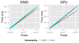
Figure 6: Execution time of SIMD and GPU of the parallel phase on GTX 560 scales linearly as image size increased. The other tested platforms showed a similar trend.

Figure 6 indicates that the parallel phase scales linearly with respect to image size. Thus, we perform polynomial fits on the parallel phase, $P_{\mathit{CPU}}$ and $P_{\mathit{GPU}}$, as a function of image width and height. Huffman decoding does not show a linear relationship with image dimension. We have observed that it varies on the complexity of the chrominance and luminance of an image, which reflects on entropy size. Figure 7 suggests a linear relationship between Huffman decoding time per pixel and entropy density. Because the encoded bitstream occupies the largest portion of a JPEG file, the density of entropy coded data can be approximated from image file size and image dimensions as

$$d=\frac{\mathit{ImageFileSize}}{w*h},$$ (3)

where $w$ is the image width, $h$ is the image height and $d$ is the image’s entropy density per pixel. We model the Huffman decoding rate, $T_{\mathit{HuffmanPerPixel}}$, using polynomial regression as a function of entropy density. The Huffman decoding time of the entire image, $T_{\mathit{Huff}}$, is approximated as follows.

$$T_{\mathit{Huff}}(w,h,d)=T_{\mathit{HuffmanPerPixel}}(d)*w*h$$ (4)

This equation assumes that entropy data is evenly distributed across an image, which we found to be a workable approximation.

The variables to our performance model are image width, height and entropy data size. We model each phase using polynomial regression up to a degree of seven. The best fit model is selected by comparing Akaike information criteria Akaike [1981]. Modelling with higher degrees is computationally possible. However, we have observed that higher degrees do not imply a more precise model, and performance may suffer from the higher prediction time required to evaluate polynomials of higher degrees.

Evaluating polynomials of high degrees at run-time showed a noticeable negative impact on the performance of the JPEG decoder. We rearranged all polynomials in Horner form Horner [1819] to reduce the number of multiplications required for polynomial evaluations. With this optimization the prediction overhead became negligible compared to the overall execution time for decoding.

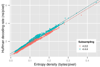
Figure 7: Huffman decoding rate on GTX 560 with respect to the density of entropy in bytes per pixel along with best-fit lines.

The overall execution time on a CPU can be expressed as a summation of the sequential phase and the parallel phase:

$$T_{\mathit{total}}=T_{\mathit{Huff}}(w,h,d)+P_{\mathit{CPU}}(w,h),$$ (5)

When we profile execution times on the GPU, OpenCL work-group sizes are alternated from 4 MCUs to 32 MCUs to find the best work-group size for a specific platform. Similar to the CPU model, the total execution time for the GPU mode is expressed a summation of Huffman decoding time and GPU execution time.

$$T_{\mathit{total}}=T_{\mathit{Huff}}(w,h,d)+P_{\mathit{GPU}}(w,h)$$ (6)

Data transfers between CPU and GPU device generate significant overhead Gregg and Hazelwood [2011]. The time collected for the GPU includes data transfer overhead and the GPU kernel computation,

$$P_{\mathit{GPU}}(w,h)=O_{w}(w,h)+T_{kernel}(w,h)+O_{r}(w,h),$$ (7)

where $O_{w}$ and $O_{r}$ are data transfer costs from the CPU to the GPU and vice versa. The input and output buffers are pinned, to achieve faster transfers Nvidia Corporation [2012].

(a) SPS

(b) Overlapped

(c) PPS

Figure 8: Heterogeneous JPEG decoding timelines of three execution models: 8(a) SPS, 8(b) overlapped Huffman decoding and GPU execution, and 8(c) PPS. Partitioning schemes are depicted proportionally; PPS achieves the highest overlap of GPU kernel execution with the sequential Huffman decoding on the CPU. Note that the last GPU invocation is shorter because the work is shared with the CPU (SIMD).

5.2 Partitioning Schemes

For reasons introduced in Section 1, Huffman decoding constitutes the non-parallelizable part of JPEG decoding, which is thus entirely executed on the CPU. Subsequent decoding steps, i.e., IDCT, upsampling and color conversion constitute the parallelizable part for which we utilize both the CPU and the GPU. For the parallelizable part, our partitioning scheme splits images horizontally such that the initial $x$ rows of the image are assigned to the GPU, and the remaining $h-x$ rows are assigned to the CPU. The value for variable $x$ is chosen such that the overall execution times for the CPU and GPU are equal, i.e., the load is equally balanced. Variable $x$ is rounded to the nearest value evenly divisible by the number of rows in an MCU. This requirement is due to libjpeg-turbo’s convention to decode images in units of MCUs. The input parameters to our partitioning schemes are the image dimensions and the image entropy, approximated by bytes/pixel derived from the image data size and the image dimensions.

5.2.1 Simple Partitioning Scheme (SPS):

The simplest approach is to parallelize the computations after Huffman decoding. CPU and GPU perform the parallel phase concurrently. Figure 8(a) illustrates the SPS partitioning scheme. The CPU first performs entropy decoding of the entire image, then partitions the resulting image data in two parts. The first part is processed by the GPU and the second part by the CPU. Data transfer commands between CPU and GPU and kernel launching commands are asynchronous calls. Hence, the CPU is allowed to continue execution after dispatching commands to the GPU. The overall execution time can be modelled as the maximum time of the two architectures.

$$T_{\mathit{total}}=max(T_{\mathit{CPU}},T_{\mathit{GPU}})$$ (8)

With the SPS model, the CPU execution time, $T_{\mathit{CPU}}$, and the GPU execution time, $T_{\mathit{GPU}}$, are expressed as

$$T_{\mathit{CPU}}(w,h) =T_{\mathit{Huff}}(w,h,d)+,T_{\mathit{disp}}(w,h-x)+P_{\mathit{CPU}}(w,x),\text{ and}$$ (9a)

$$T_{\mathit{GPU}}(w,h) =T_{\mathit{Huff}}(w,h,d)+P_{\mathit{GPU}}(w,h-x),$$ (9b)

where $x$ is the number of rows assigned to the CPU, and $T_{\mathit{disp}}$ is the amount of time the CPU spends on the OpenCL kernel invocation. $P_{\mathit{GPU}}$ includes kernel execution time and data transfer overhead. The workload is considered well-balanced when the parallel parts on both architectures achieve the same execution time.

$$f(x)=T_{\mathit{disp}}(w,h-x)+P_{\mathit{CPU}}(w,x)-P_{\mathit{GPU}}(w,h-x)$$ (10)

The only unknown variable is the number of rows assigned to the CPU, i.e., $x$. When $f(x)$ become zero, the execution time is balanced. This problem is equivalent to the root solving problem. At run-time, the root can be estimated using Newton’s method,

$$x_{n+1}=x_{n}-\frac{f(x_{n})}{f^{\prime}(x_{n})},$$ (11)

where $x_{n}$ is the initial partitioning height to the CPU, $x_{n+1}$ is the new height approximation, $f(x_{n})$ is given as Equation (10), and $f^{\prime}(x_{n})$ is the first derivation. Newton’s method is performed recursively until no better partition can be found. The GPU computes the parallel phase on the sub-image of size $w$ by $h-x$, while the CPU computes the remaining $x$ image rows.

5.2.2 Pipelined Partitioning Scheme (PPS):

The GPU is underutilized during the Huffman decoding stage in SPS. We have demonstrated in Section 4.5 that sequential Huffman decoding can be parallelized with GPU kernel execution. Entropy data for the CPU can be decoded simultaneously with GPU computations as illustrated in Figure 8(b). The concurrent execution happens after the Huffman decoding part for the GPU. The total execution time on each architecture can be modelled as follows.

$$T_{\mathit{CPU}} =T_{\mathit{Huff}}(w,h,d)+P_{\mathit{CPU}}(w,x)+T_{\mathit{disp}}(w,h-x)$$ (12a)

$$T_{\mathit{GPU}} =T_{\mathit{Huff}}(w,h-x,d)+P_{\mathit{GPU}}(w,h-x)$$ (12b)

This partitioning scheme balances GPU execution with the sum of OpenCL dispatching time, entropy decoding time for the CPU part and the computation time of the parallel part on the CPU.

$$\begin{split}f(x)=&T_{\mathit{disp}}(w,h-x)+T_{\mathit{Huff}}(w,h,d)+P_{\mathit{CPU}}(w,x)\\ &-P_{\mathit{GPU}}(w,h-x)\end{split}$$ (13)

Similar to SPS, we use Newton’s method to approximate variable $x$ at run-time.

Further parallelism can be achieved by pipelining the GPU kernel executions with this partitioning scheme. Figure 8(c) shows an execution timeline of PPS. The parallel part for the first image chunk (Huffman 1) is started on the GPU immediately after it has been transferred from the CPU.

$$T_{\mathit{CPU}} =T_{\mathit{Huff}}(w,h,d)+P_{\mathit{CPU}}(w,x)+T_{\mathit{disp}}(w,h-x)$$ (14a)

$$T_{\mathit{GPU}} =T_{\mathit{Huff}}(w,c,d)+P_{\mathit{GPU}}(w,h-x)$$ (14b)

In the above equation, $c$ is the number of image rows per chunk decoded on the GPU. The chunk size has been determined through profiling as explained in Section 4.5. The number of rows per chunk can be calculated by chunk size divided by image width. Therefore, the partitioning equation becomes

$$\begin{split}f(x)=&T_{\mathit{Huff}}(w,h-c,d)+P_{\mathit{CPU}}(w,x)+T_{\mathit{disp}}(w,h-x)\\ &-P_{\mathit{GPU}}(w,h-x),\end{split}$$ (15)

where $h-c$ denotes the remaining rows in an image after the first chunk.

Our Huffman decoding time estimation model assumes a uniform entropy distribution across an image. However, the density of entropy data is unlikely to be evenly distributed in practice. Using the Huffman decoding time model to estimate the time for a certain chunk is often imprecise because the average density and the actual density of the chunk are mismatched. We compensate the error by re-partitioning. Throughout the computation, we keep records of the actual Huffman decoding times. Before entropy decoding of the last GPU chunk, workload distribution is re-calculated. At this point, one GPU chunk and the CPU partition remain unprocessed. Thus, a modification of Equation (13) can be used,

$$\begin{split}f(x)=&T_{\mathit{disp}}(w,h^{\prime}-x^{\prime})+T_{\mathit{Huff}}(w,h^{\prime},d^{\prime})+P_{\mathit{CPU}}(w,x^{\prime})\\ &-P_{\mathit{GPU}}(w,h-x)-P_{prevGPU},\end{split}$$ (16)

where $h^{\prime}$ is the unprocessed height, $x^{\prime}$ is the new height allocated to the GPU, and $d^{\prime}$ is the new density rate. The previous kernel execution may not complete by the time of re-partitioning. $T_{prevGPU}$ is an estimated remaining time from the previous GPU kernel invocation that potentially influences the new partitioning scheme. The remaining height, $h^{\prime}$, is known at run-time. The only unknown variable to be solved at run-time, is $x^{\prime}$.

We estimate the total Huffman decoding time using Equation (4), and the actual Huffman decoding time of previous chunks are known at run-time. Figure 7 implies a linear proportional relationship between an image dimension and Huffman decoding time. The new density is calculated using the ratio of the remaining Huffman time and the image height.

$$d^{\prime}=\frac{\mathit{HuffmanDecodingTimeRatio}}{\mathit{ImageHeightRatio}}*d,$$ (17)

Above, $HuffmanDecodingTimeRatio$ is the ratio of the remaining decoding time to the estimated total decoding time, and $ImageHeightRatio$ is the ratio of unprocessed height to the total image height. When the ratio of the remaining Huffman time is greater than the height ratio, the remaining part of an image consists of more detail. It indicates that the entropy data rate becomes denser and more workload should be allocated to the GPU. Otherwise, the entropy data rate becomes less dense, and more workload should be allocated to the CPU.

Even though Figure 8(c) shows a small gain compared to Figure 5(b), this approach actually yields large improvements on a hardware configuration where the CPU is more powerful than the GPU.

6 Experimental Results

We conducted an extensive experimental evaluation on six versions of the JPEG decoder, namely the sequential version, SIMD, GPU, pipelined GPU, SPS and PPS, on three representative platforms specified in Table 1. All file I/O instructions were disabled to minimize time variations that do not reflect the actual performance of the algorithm. To demonstrate the effectiveness of our implementation, we used two chroma subsamplings, i.e., 4:2:2 and 4:4:4. The other subsamplings are decoded in a similar manner as 4:2:2 images. For the performance evaluation we used a new set of images that does not share any images with the training set. Our image test-set consists of fourteen images from CorpusNielsFrohling and three self-taken images. These images are cropped to various sizes summing up to the total of 3597 images for each subsampling.

Machine name	GT 430	GTX 560	GTX 680
CPU model	Intel i7-2600k	Intel i7-2600k	Intel i7-3770k
CPU frequency	3.4 GHz	3.4 GHz	3.5 GHz
No. of CPU cores	4	4	4
GPU model	NVIDIA GT 430	NVIDIA GTX 560Ti	NVIDIA GTX 680
GPU core frequency	700 MHz	822MHz	1006MHz
No. of GPU cores	96	384	1536
GPU memory size	1024 MB	1024 MB	2048 MB
Compute Capability	2.1	2.1	3.0
Ubuntu version	11.04	12.04	11.04
Linux Kernel	2.6.38	3.5.0	2.6.38
GCC version	4.5.2	4.6.3	4.5.2

Table 1: Hardware Specifications.

6.1 OpenCL Kernel Execution

Figure 9 depicts a break-down of execution times for the sequential CPU, SIMD and GPU modes. The y-axis is normalized with respect to SIMD execution times. Our GPU computations on all tested architectures surpass the sequential CPU execution. For this specific image size, the GPU computation was able to reduce 35.5% and 40.8% of the overall execution time on GTX 560 and GTX 680 respectively. The kernel execution from IDCT to color conversion was 10x faster than the SIMD execution on the GTX 560 and 13.7x faster on the GTX 680. However, taking data transfer overhead into account, the performance improvements were reduced to 2.6x and 4.3x.

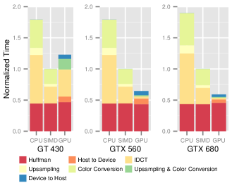
Figure 9: Decoding time normalized with respect to JPEG decompression in SIMD mode. The decoded image’s dimension is 2048x2048 with 4:2:2 subsampling. Shown are the execution time break-downs of libjpeg-turbo’s sequential JPEG decoder on the CPU, SIMD execution on a CPU with libjpeg-turbo, and our GPU execution.

It follows from Fig. 9 that performance improvements are not guaranteed by migrating computations exclusively to a GPU. GT 430, consisting of 96 cores, is the weakest GPU among the three representative machines. The experimental result on the 2048x2048 image showed a 23% slow-down compared to SIMD execution on an Intel i7. The kernel execution shows a 27% slower data transfer between CPU and GPU.

6.2 Heterogeneous JPEG Decoding Performance

We evaluated our heterogeneous JPEG decompression models with respect to the SIMD-version of libjpeg-turbo. Figure 10 shows the average speedups with standard deviation bars as image size increased. Due to space limitations, we only provide the results for 4:4:4 subsampling. A similar trend was observed for 4:2:2 subsampling. Table 2 and Table 3 summarize the performances of 4:2:2 and 4:4:4 subsampling respectively.

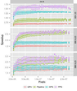
Figure 10: Average speedups over libjpeg-turbo’s SIMD execution with respect to image size in pixels on the three representative machines. The error bar represents standard deviation.

Mode	GT 430	GTX 560	GTX 680
GPU	$0.72\pm 5.35\%$	$1.59\pm 7.50\%$	$1.94\pm 12.94\%$
Pipeline	$0.92\pm 13.67\%$	$2.19\pm 20.21\%$	$2.33\pm 20.75\%$
SPS	$1.31\pm 9.54\%$	$1.81\pm 10.13\%$	$2.04\pm 15.15\%$
PPS	$1.54\pm 10.93\%$	$2.34\pm 15.19\%$	$2.52\pm 17.08\%$

Table 2: Average speedup and coefficient of variation over SIMD execution when decoding 4:2:2 subsampled images.

Mode	GT 430	GTX 560	GTX 680
GPU	$0.66\pm 5.82\%$	$1.49\pm 5.87\%$	$1.81\pm 10.84\%$
Pipeline	$0.83\pm 13.48\%$	$2.14\pm 19.97\%$	$2.26\pm 19.48\%$
SSP	$1.27\pm 8.62\%$	$1.76\pm 8.12\%$	$1.94\pm 12.55\%$
PPS	$1.50\pm 10.46\%$	$2.34\pm 14.33\%$	$2.45\pm 15.02\%$

Table 3: Average speedup and coefficient of variation over SIMD execution when decoding 4:4:4 subsampled images.

PPS achieves the highest performance on all machines. It attains average speedups of 1.5x, 2.3x and 2.5x over SIMD mode and 3.1x, 4.8x and 5.2x over sequential execution on GTX 430, GTX 560 and GTX 680 respectively. The highest-recorded speedups were 4.2x faster than SIMD and 8.5x faster than sequential execution on GTX 680. PPS does not show a signification improvement over pipelined GPU execution on GTX 560 and GTX 680 because most GPU kernel executions were sufficiently fast to hide within the Huffman decompression time. Therefore, only a small amount of workload was allocated to the CPU, and a small improvement was achieved.

On GT 430, the GPU mode and the pipelined GPU execution mode failed to surpass SIMD. As a result, both of our partitioning schemes distributed the larger partition to the CPU. Despite the slow GPU, the cooperative CPU-GPU executions achieved speedups over libjpeg-turbo’s SIMD mode.

The pipelined execution is always faster than a single large GPU kernel invocation because entropy is decoded simultaneously with a GPU computation to reduce the hardware idle time. When the decoded image has a size smaller than the pre-determined chunk size, the image is executed as one GPU kernel invocation. Therefore, no improvement is shown over the normal GPU mode.

It should be noted that the GTX 680 has larger coefficients of variation than the other machines. This fluctuation reflected the contribution of Huffman decoding time to the speedup calculation. An image with larger entropy data takes longer time to decode. As a result, the overall speedup becomes smaller than an image with sparser entropy. The faster GPU is more sensitive to the change. Therefore, GTX 680 suffered the highest impact from a small change in Huffman decoding time compared to the other tested machines.

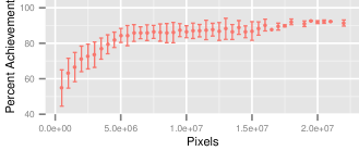
Figure 11: Speedup Comparison of PPS execution to the maximum achievable speedup on GTX 680. The points represent the mean percent achieved along with standard deviation bars.

According to Amdahl’s law, the maximum attainable speedup is restricted by the sequential portion of the program. Equation (18) states the theoretical speedup assuming an infinite number of processors.

$$\mathit{Speedup}=\frac{T_{\mathit{total}}}{T_{\mathit{total}}*(1-P)}$$ (18)

$P$ is the fraction of the parallelizable portion of the program, and $1-P$ is the serial portion, which in this case, is entropy (Huffman) decoding. Thus, the maximum achievable speedup over libjpeg-turbo’s SIMD-version can be written as

$$\mathit{Speedup}=\frac{T_{\mathit{total}}}{T_{\mathit{Huff}}},$$ (19)

where $T_{\mathit{total}}$ is the decoding time of the SIMD-version. We compared the speedup of our approach to the theoretically attainable speedup in Figure 11. PPS stabilizes at an average speedup of 88% and attains its peak at 95% of the theoretically attainable speedup. For small images, the speedup was slightly higher than half of the maximum attainable speedup because these images were partitioned into few chunks for pipeline execution.

Consequently, less work was executed in parallel with entropy decoding. Increasing the number of chunks would result in a lack of data for GPU computation. As image size increases, an image is split into more chunks, and thus, less work of the parallelizable phase is visible to the user.

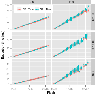
Figure 12: The average CPU and GPU execution time with standard deviation during parallel executions are balanced indicating balance workload between architectures.

Figure 12 shows execution times of the CPU and the GPU during the parallel execution. In the simple heterogeneous execution, the entropy decoding time was omitted from CPU time as it is sequentially executed on the GPU. Similarly, the entropy decoding of the first image chunk of the pipelined execution was omitted. GPU and CPU shared similar execution times indicating well-balanced loads. The main contribution to the variation in the pipelined heterogeneous mode is Huffman decoding time.

7 Related Work

DCT and IDCT algorithms are computationally intensive, but exhibit a high potential for parallelism. Various image processing algorithms, including DCT and IDCT, have been implemented for a GPU architecture by Yang et al. Yang et al. [2008]. The authors utilized CUDA and applied CUFFT Nvidia Developer [2008], a CUDA fast Fourier transform (FFT) library, to perform DCT and IDCT. However, extracting DCT from FFT introduces extra computational overhead. The NVIDIA GPU Computing SDK provides DCT and IDCT sample code to demonstrate GPU programming. The kernel’s input and output data type are float. In contrast to our implementation, the input buffer to our kernel is an array of short and the output buffer is an array of unsigned character. These data types are vectorized to minimize global memory transfer overhead. Moreover, we combine dequantization, IDCT and color conversion in a single kernel to reduce data communication.

A task-parallel implementation of JPEG decoding using libjpeg-turbo has been explored by Hong et al. J. Hong et al. [2012]. Fork/join parallelism is applied to decode an image on CPU cores simultaneously. GPUJPEG GPUJPEG: JPEG compression and decompression accelerated on GPU [retrieved Feb. 2013] is an open source JPEG image compression and decompression library for NVIDIA designed for real-time video. Tasks for image decoding are divided between a CPU and GPUs where the CPU performs file I/O operations and Huffman decoding while the GPUs compute IDCT and color conversion. The GPU kernel is, yet, optimized. Although the computationally intensive tasks are parallelized on the GPUs, the entire process is done serially. On the contrary, we minimize hardware idle time by utilizing software pipelines and distributing workload across CPU and GPU.

Research on heterogeneous computing is receiving attention in high performance computing. Shee et al. Shee et al. [2008] conducted a case study on JPEG encoders on Application Specific Instruction-set Processors (ASIPs). They evaluated two parallel programming patterns: master-slave and pipeline. The master-slave model utilized task management and data-parallelism. In the pipelined model, different ASIP processors were responsible for different stages of JPEG encoding. L. Chen et al. Chen et al. [2012] proposed a similar idea for MapReduce applications. The authors developed two scheduling schemes, namely master-slave and pipeline model, on integrated CPU-GPU systems. Data-parallelism and pipeline-parallelism were utilized separately. The Qilin framework Luk et al. [2009] and CHC framework Lee et al. [2012] showed possibilities of a cooperative CPU-GPU computation of a CUDA application. Both frameworks dynamically partitioned the workloads using their profiling based partitioning models. Qilin used an empirical approach recording new execution to a database while CHC applied a heuristic approach. The partitioning schemes were designed for CUDA applications and only supported data-parallelism. The CAP scheduler Wang et al. [2013] supports dynamic workload scheduling on CPU-GPU systems. Profiling and workload partitioning are performed at run-time. CAP profiles a small portion of the workload, verifies the accuracy of the ratio and then uses the ratio for the remaining of workload. Although it can effectively partition workload, it only supports data-parallelism. Our proposed partitioning scheme, in comparison, is designed specifically for JPEG decoder. The workload is partitioned without user intervention, and the CPU and the GPU jointly perform the decoding tasks cooperating data-, task- and pipeline-parallelism.

8 Conclusions

We have introduced a novel JPEG decoding scheme for heterogeneous architectures consisting of a CPU and an OpenCL-programmable GPU. Our method employs an offline profiling step to determine the performance of a system’s CPU and GPU with respect to JPEG decoding. We apply multivariate polynomial regression analysis to derive closed forms that characterize the performance of a given CPU-GPU combination. Image entropy and the image dimensions are the sole parameters for our performance model. At run-time, closed forms are evaluated for a given image to estimate execution times and load-balance the decoding workload between the CPU and the GPU. Our run-time partitioning scheme exploits task, data and pipeline parallelism by scheduling the non-parallelizable entropy decoding task on the CPU, whereas IDCT, color conversion and upsampling are conducted on both the CPU and the GPU. Our kernels have been optimized for GPU memory hierarchies.

We have implemented the proposed method in the context of the libjpeg-turbo library, which is an industrial-strength JPEG encoding and decoding engine. Irrespective of the GPU’s computational power, our heterogeneous partitioning scheme always achieves an improvement over the SIMD-version of libjpeg-turbo. The results show speedups up to 8.5x over the sequential version and up to 4.2x over the SIMD version of libjpeg-turbo. We have shown that our approach achieves up to 95% of the theoretically attainable speedup, with an average of 88%. With the availability of GPU accelerators on desktops and embedded devices such as tablets and smartphones, heterogeneous JPEG image decompression will enhance image viewing experiences ranging from personal photos to very large image applications in medical imaging and astronomy.

References

- Akaike [1981] H. Akaike. Likelihood of a model and information criteria. Journal of Econometrics, 16(1):3 – 14, 1981.
- Alexa Top 500 Global Sites [retrieved Feb. 2013] Alexa Top 500 Global Sites. http://www.alexa.com/topsites, retrieved Feb. 2013.
- Beaver et al. [2010] D. Beaver, S. Kumar, H. C. Li, J. Sobel, P. Vajgel, and F. Inc. Finding a needle in haystack: Facebook’s photo storage. In Proc. of OSDI, 2010.
- Capocelli et al. [1988] R. Capocelli, L. Gargano, and U. Vaccaro. On the characterization of statistically synchronizable variable-length codes. Information Theory, IEEE Transactions on, 34(4):817–825, 1988.
- Chen et al. [2012] L. Chen, X. Huo, and G. Agrawal. Accelerating MapReduce on a coupled CPU-GPU architecture. In Proc. SC’12. IEEE Press, 2012.
- GPUJPEG: JPEG compression and decompression accelerated on GPU [retrieved Feb. 2013] GPUJPEG: JPEG compression and decompression accelerated on GPU. http://sourceforge.net/p/gpujpeg/home/Home/, retrieved Feb. 2013.
- Gregg and Hazelwood [2011] C. Gregg and K. Hazelwood. Where is the data? Why you cannot debate CPU vs. GPU performance without the answer. In Proc. of ISPASS’11, pages 134–144, 2011.
- Horner [1819] W. G. Horner. A new method of solving numerical equations of all orders, by continuous approximation. Philosophical Transactions of the Royal Society of London, 109:pp. 308–335, 1819.
- Image Compression Benchmark [retrieved July 2013] Image Compression Benchmark. http://www.imagecompression.info/test_images/, retrieved July 2013.
- Instagram Press Center [retrieved Jun. 2013] Instagram Press Center. http://instagram.com/press/, retrieved Jun. 2013.
- J. Hong et al. [2012] J. Hong et al. Design, implementation and evaluation of a task-parallel JPEG decoder for the libjpeg-turbo library. International Journal of Multimedia and Ubiquitous Engineering, 7(2), 2012.
- Klein and Wiseman [2003] S. T. Klein and Y. Wiseman. Parallel Huffman decoding with applications to JPEG files. Computer J., 46:487–497, 2003.
- Lee et al. [2012] C. Lee, W. W. Ro, and J.-L. Gaudiot. Cooperative heterogeneous computing for parallel processing on CPU/GPU hybrids. In Interaction between Compilers and Computer Architectures. IEEE, 2012.
- Libjpeg [retrieved Jun. 2013] Libjpeg. http://libjpeg.sourceforge.net/, retrieved Jun. 2013.
- Libjpeg Turbo [retrieved Jun. 2013] Libjpeg Turbo. http://sourceforge.net/projects/libjpeg-turbo, retrieved Jun. 2013.
- Luk et al. [2009] C.-K. Luk, S. Hong, and H. Kim. Qilin: exploiting parallelism on heterogeneous multiprocessors with adaptive mapping. In Proc. of MICRO 42. ACM, 2009.
- Nvidia Corporation [2012] Nvidia Corporation. OpenCl programming guide for the CUDA architecture, version 4.2. Technical report, 2012.
- Nvidia Developer [2008] Nvidia Developer. CUDA CUFFT library manual version 5.0, 2008.
- Pennebaker and Mitchell [1992] W. B. Pennebaker and J. L. Mitchell. JPEG Still Image Data Compression Standard. Kluwer, 1st edition, 1992.
- Poynton [Retrieved July 2013] C. Poynton. Chroma subsampling notation. Retrieved July 2013.
- Shee et al. [2008] S. Shee, A. Erdos, and S. Parameswaran. Architectural exploration of heterogeneous multiprocessor systems for JPEG. IJPP, 36(1):140–162, 2008.
- The WebKit Open Source Project [retrieved Jun. 2013] The WebKit Open Source Project. http://www.webkit.org/, retrieved Jun. 2013.
- Wallace [1991] G. K. Wallace. The JPEG still picture compression standard. Communications of the ACM, pages 30–44, 1991.
- Wang et al. [2013] Z. Wang, L. Zheng, Q. Chen, and M. Guo. CAP: co-scheduling based on asymptotic profiling in CPU+GPU hybrid systems. In Proc. of PMAM’13, pages 107–114. ACM, 2013.
- Yang et al. [2008] Z. Yang, Y. Zhu, and Y. Pu. Parallel image processing based on CUDA. In Proc. of CSSE’08. IEEE Computer Society, 2008.
- Yukihiro et al. [1988] A. Yukihiro, A. Takeshi, and M. Nakajima. A fast DCT-SQ scheme for images. IEICE TRANSACTIONS (1976-1990), 71(11):1095–1097, 1988.