UOSTP 130901

Multi-faced Black Janus and Entanglement

Dongsu Bak, and Hyunsoo Min

Physics Department, University of Seoul, Seoul 130-743, Korea

(dsbak@uos.ac.kr, hsmin@dirac.uos.ac.kr)

Abstract

To the second order of the deformation parameter, we construct the black brane solutions, which are dual to the multiple interface deformations of conformal field theories. We compute their thermodynamic quantities from the gravity and the field theory sides, and find a precise agreement, confirming the validity of the AdS/CFT correspondence. The correlation of two separate interfaces induces a Casimir energy and an interesting form of correlated entropy contribution. We comment on the properties of the interface lattice system too.

1 Introduction

The Janus solutions [1] in various supergravity theories, which are dual to the interface conformal field theories (ICFT), provide well-controlled deformations of the AdS/CFT correspondence [2, 3, 4]. In the simplest examples, the bulk gravity is described by the Einstein-scalar theory with a negative cosmological constant. One uses the AdS_d slicing of the AdS_d+1 and makes the massless scalar field dependent on the slicing coordinate. The scalar field approaches two different constant values at the boundary of the space, which results in a jump of the coupling through the interface of the boundary CFT. Out of the original SO$(d,2)$ conformal symmetries of the CFT, this simple interface deformation preserves one lower dimensional conformal symmetries, SO$(d-1,2)$. See Refs. [5]-[19] for further development and other related studies.

Recently in Ref. [15], the black Janus solution in three dimensions was considered, which is the Janus deformation of the well known BTZ black hole solution [20]. The corresponding boundary theory is given by the simple interface deformation of the CFT on ${R}^{1,1}$. Strictly speaking, the black Janus geometry is dual to the finite-temperature version of the ICFT. It was found that the interface system carries a zero-temperature entropy whose exponential counts the degeneracy of the ground states. Using the solution, the thermodynamic quantities of this ICFT can be calculated based on the dictionary of the AdS/CFT correspondence. In the field theory side, these results were reproduced, via the so-called conformal perturbation theory, to the second order of the deformation parameter.

In this paper, we would like to extend the above analysis to the general multiple interface system. We shall approach the problem by a perturbative construction of solutions. The zeroth order of the perturbation theory begins with the BTZ black hole solution. Our background is dependent upon a single (temperature) scale reflecting the conformal invariance of the underlying system. Around the BTZ background, we shall consider general static perturbation of the Einstein-scalar theory. The scalar perturbation begins with the term of $O(\gamma)$ where $\gamma$ is our deformation parameter counting the order of the perturbation series. The order of the general scalar perturbation terms is counted as $\gamma^{2n+1}$ with $n\geq 0$. On the other hand, the perturbation in the geometric part begins with terms of $O(\gamma^{2})$ and the order of its general perturbation is counted as $\gamma^{2n+2}$ with $n\geq 0$.

We shall first solve the leading order term of the scalar part, which satisfies a linear partial differential equation. One can show that the most general boundary condition for the scalar term is that its values should approach piecewise constants at the boundary of the space. For a single interface, the solution of the equation was already constructed in [15]. The general solution can be given by the linear superposition of each single-interface solution whose center is located at an arbitrary position of the boundary spatial direction. The leading order of the geometric part is reduced to linear differential equations with source terms determined by the above solution of the scalar part. The source is consisting of two different kinds of terms. One is from the diagonal contributions of each scalar solution for each interface. The solution with a source term of this kind is known in Ref. [15]. The other kind is consisting of the off-diagonal contributions of a set of scalar solutions from two different interfaces.

Up to the translational freedom in the boundary spatial direction, the source term and the corresponding equations are characterized by the separation distance $l$ of the two interfaces. The existence of the extra scale $l$ breaks the underlying conformal invariance in a rather clear manner. Hence solving this geometric part becomes highly nontrivial. However, it should be in principle possible to find solutions since we are dealing with linear partial differential equations with specified source terms. To solve those nontrivial partial differential equations, we adopt a suitable ansatz even though its structure is not completely justified. We shall find explicit forms of solutions (with a freedom of adding homogeneous solutions), which satisfy all of the required physical properties. Since the procedure of finding solutions is nontrivial, we shall present its details below.

Once the full solution is constructed, one may study the properties of the multiple interface system using the dictionary of the AdS/CFT correspondence. We first note the diagonal and off-diagonal parts of the solutions involve specific homogeneous terms. We shall show that these homogeneous solutions are related to the coordinate transformations that preserve the original BTZ form of the metric to the $O(\gamma^{2})$. Next for the above mentioned solutions, we shall construct the Fefferman-Graham form of the metric and identify the energy momentum tensor of the boundary field theory using the holographic dictionary [21]. In addition to the energy momentum contribution of the undeformed CFT, we find the Casimir energy and pressure coming from any pairs of two interfaces. Using the boundary-horizon map in [15, 22], we compute the horizon length of the multiple interface system and identify the entropy of the interface geometry.

The dual boundary field theory is given by the multiple-interface deformation of the CFT on $R^{1,1}$. Each interface is realized as a jump of the coupling where the corresponding marginal operator is the Lagrange density operator. Using the conformal perturbation theory, we shall compute the free energy up to the $O(\gamma^{2})$ in the strong coupling limit. Once the free energy is obtained, the energy and the entropy follow from the thermodynamic relations. We shall find the agreement of these two independent computations in the strong coupling limit. We shall also comment on the properties of interface lattice [26, 27, 28, 29] and discuss the zero temperature limit of the multiple interface system.

In Section 2, we review the Janus and black Janus solutions in three dimensions, which are relevant for the subsequent discussions. We also present the global Janus solution which is dual to the interface deformation of the CFT on $S^{1}\times R$. Using the method of the holographic entanglement entropy, we identify the entropy of the interface on the circle $S^{1}$. Section 3 discusses the perturbative setup for the general static solutions around the BTZ black hole background. In Section 4, we discuss the leading scalar part of solutions for the general interface system. Section 5 deals with the construction of the geometric part of solution to the $O(\gamma^{2})$. Section 6 presents the (finite temperature) physics of the double interfaces. The field theoretic treatment of the double interface system is considered in Section 7. Section 8 deals with the properties of the general multiple interface systems including the interface lattice. In Section 9, we take the zero temperature limit of the solutions. Last section is devoted to the discussions and concluding remarks. Various technical details are collected in Appendices.

2 Janus system and some known solutions

We begin with the 3d Einstein scalar system

$$S={1\over 16\pi G}\int d^{3}x\sqrt{g}\left(R-g^{ab}\partial_{a}\phi\partial_{b}\phi+2\right),$$ (2.1)

which can be consistently embedded into the type IIB supergravity theory [13]. Here we set the AdS radius $R_{AdS_{3}}$ to be unity for simplicity and recover it whenever it is necessary. We are interested in the most general geometries for which asymptotic values of the scalar field are allowed to vary. The Einstein equation reads

$$R_{ab}+2g_{ab}=\partial_{a}\phi\partial_{b}\phi$$ (2.2)

and the scalar equation of motion is given by

$$\partial_{a}(\sqrt{g}g^{ab}\partial_{b}\phi)=0.$$ (2.3)

Any resulting solutions involving nontrivial scalar field will be deformations of the well known AdS${}_{3}\times S^{3}$ background [30].

2.1 Janus solutions

For the static Janus solution, we take an ansatz for the three dimensional metric and the scalar field in the following form

$$ds^{2}=dr^{2}+f(r){-dt^{2}+d{\xi}^{2}\over\xi^{2}},\quad\quad\phi=\phi(r).$$ (2.4)

Using this ansatz, it was found that the solution of the equations of motion (2.2) and (2.3) is given by [13]

$$f(r)={1\over 2}\Big{(}1+\sqrt{1-2\gamma^{2}}\cosh 2r\Big{)}$$ (2.5)

and

$$\phi(r)=\phi_{0}+{1\over\sqrt{2}}\log\left({1+\sqrt{1-2\gamma^{2}}+\sqrt{2}\gamma\tanh r\over 1+\sqrt{1-2\gamma^{2}}-\sqrt{2}\gamma\tanh r}\right).$$ (2.6)

Without loss of generality, we may set $\phi_{0}=0$. The Janus solution holographically realizes an ICFT where two CFTs defined on $1+1$ dimensional half spaces are glued together over a $0+1$ dimensional interface. The conformal boundary of the metric (2.4) has three components. As $r\to\pm\infty$ and finite $\xi>0$, we can strip off the $1/\xi^{2}$ factor, and the corresponding boundary components are two copies of $R_{+}\times R$ spanned by $\xi,t$. Note that the scalar approaches two constant values at these boundaries

$$\lim_{r\to\pm\infty}\phi(r)=\pm{1\over\sqrt{2}}\log\left({1+\sqrt{1-2\gamma^{2}}+\sqrt{2}\gamma\over 1+\sqrt{1-2\gamma^{2}}-\sqrt{2}\gamma}\right).$$ (2.7)

The value of the scalar on the boundary is dual to a coupling (modulus) of the two dimensional CFT. The third boundary component is at $\xi=0$, which is the boundary of the AdS₂ factor. This describes the interface where the two half planes are glued together. Hence the dual CFT is an ICFT where two CFTs defined on a half line are at different points in their coupling space.

After introducing an angular coordinate $\mu$ by

$$dr=\sqrt{f(r)}d\mu,$$ (2.8)

we can present the above solution in the form [13]

$$ds_{3}^{2}=f(\mu)\left(d\mu^{2}+{-dt^{2}+d{\xi}^{2}\over\xi^{2}}\right),\quad\quad\phi=\phi(\mu)$$ (2.9)

where

$$f(\mu) = \frac{\kappa_{+}^{2}}{{\rm sn}^{2}(\kappa_{+}(\mu+\mu_{0}),k^{2})}=\frac{\kappa_{+}^{2}{\rm dn}^{2}(\kappa_{+}\mu,k^{2})}{{\rm cn}^{2}(\kappa_{+}\mu,k^{2})},$$ (2.10)

$$\phi(\mu) = \frac{1}{\sqrt{2}}\ln\left(\frac{{\rm dn}(\kappa_{+}(\mu+\mu_{0}),k^{2})-k{\rm cn}(\kappa_{+}(\mu+\mu_{0}),k^{2})}{{\rm dn}(\kappa_{+}(\mu+\mu_{0}),k^{2})+k{\rm cn}(\kappa_{+}(\mu+\mu_{0}),k^{2})}\right)$$ (2.11)

$$= \frac{1}{\sqrt{2}}\ln\left(\frac{1+k\,{\rm sn}(\kappa_{+}\mu,k^{2})}{1-k\,{\rm sn}(\kappa_{+}\mu,k^{2})}\right)$$

with

$$\kappa^{2}_{\pm}\equiv\frac{1}{2}(1\pm\sqrt{1-2\gamma^{2}}),$$ (2.12)

$$k^{2}\equiv\kappa^{2}_{-}/\kappa^{2}_{+}={\gamma^{2}\over 2}+O(\gamma^{4}),$$ (2.13)

$$\mu_{0}\equiv K(k^{2})/\kappa_{+}=\frac{\pi}{2}\left(1+\frac{3}{8}\gamma^{2}+O(\gamma^{4})\right).$$ (2.14)

This describes Janus deformation of the Poincare patch geometry.

For the deformation of the global AdS, we need to replace the AdS₂ part in (2.4) and (2.9) by the global AdS₂ leading to the solution

$$ds_{3}^{2}=f(\mu)\left(d\mu^{2}+{d{\lambda}^{2}-dt^{2}\over\cos^{2}\lambda}\right),\quad\quad\phi=\phi(\mu),$$ (2.15)

where the coordinate $\lambda$ is ranged over $[-\pi/2,\pi/2]$. The constant time slice takes a shape of a disk whose boundary is consisting of two half circles with $\mu=\pm\mu_{0}$. Hence the boundary spacetime corresponds to $S^{1}\times R$ on which the ICFT is defined. We parameterize the circle $S^{1}$ by angle $\theta$ defined by

$$\theta=\left[\begin{array}[]{cl}\pi/2-\lambda&{\rm for}\ \mu=\mu_{0},\\ \lambda-\pi/2&{\rm for}\ \mu=-\mu_{0}.\end{array}\right.$$ (2.18)

For the undeformed case with $\phi=0$, the metric takes a form

$$ds_{3}^{2}={1\over\cos^{2}\mu}\left(d\mu^{2}+{d{\lambda}^{2}-dt^{2}\over\cos^{2}\lambda}\right)$$ (2.19)

where $\mu\in[-\pi/2,\pi/2]$. After taking the coordinate transformation,

$$\cosh\rho={1\over\cos\mu\cos\lambda}\,,\ \ \ \cos\theta=\sin\lambda\,\coth\rho\,,$$ (2.20)

one is led to the usual form of the metric

$$ds^{2}=-\cosh^{2}\rho dt^{2}+d\rho^{2}+\sinh^{2}\rho d\theta^{2}\,,$$ (2.21)

where $\theta\in[-\pi,\pi]$.

The global Janus background is dual to the interface CFT on $S^{1}\times R$. Using the standard holographic dictionary, the energy density and the pressure of the ICFT can be identified as

$${\cal E}=p=-\frac{c}{12}\,\frac{1}{2\pi},$$ (2.22)

where we have used the general fact

$$\frac{R_{AdS_{3}}}{4G}=\frac{c}{6}.$$ (2.23)

Note that these quantities are independent of the Janus deformation parameter and agree with the well known results for the CFT on $S^{1}\times R$ where the circle size is set to be $2\pi$.

2.2 Entanglement entropy of global Janus

A useful observable in the ICFT is the entanglement entropy which is defined as follows. The space on which the CFT is living is divided into two regions ${\cal A}$ and ${\bar{\cal A}}$. The total Hilbert space of states $H$ is expressed by the product $H=H_{\cal A}\otimes H_{\bar{\cal A}}$, where $H_{{\cal A}}$ ($H_{\bar{\cal A}}$) is supported on ${\cal A}$ (${\bar{\cal A}}$). A reduced density matrix can be defined by tracing over all states in ${\bar{\cal A}}$,

$$\rho_{\cal A}={\rm tr}_{{\bar{\cal A}}}\rho\,,$$ (2.24)

where $\rho$ is the density matrix of the total system. At zero temperature, one takes $\rho$ to be the projector on the ground state. The entanglement entropy associated with the region ${\cal A}$ is then defined as

$$S_{\cal A}=-{\rm tr}_{{\cal A}}\rho_{\cal A}\log\rho_{\cal A}\,.$$ (2.25)

A holographic prescription to calculate the entanglement entropy in spaces which are asymptotic to AdS_d+1 was presented in [31, 32]. We denote the boundary of the region ${\cal A}$ by $\partial{\cal A}$. A static minimal surface ${\Sigma}_{\cal A}$ extends into the AdS_d+1 bulk and ends on $\partial{\cal A}$ as one approaches the boundary of AdS_d+1. The holographic entanglement entropy can then be calculated as

$$S_{\cal A}={{\rm Area}({\Sigma}_{\cal A})\over 4G_{d+1}},$$ (2.26)

where ${\rm Area}({\Sigma}_{\cal A})$ denotes the area of the minimal surface ${\Sigma}_{\cal A}$ and $G_{d+1}$ is the Newton constant for AdS_d+1 gravity.

The minimal surface is a space-like geodesic connecting the points in the constant-time slicing given by

$$dr^{2}+{f(r)\over\cos^{2}\lambda}d\lambda^{2}\,.$$ (2.27)

The geodesic to compute the entanglement entropy chooses the $\lambda$ coordinate as constant $\lambda=\pi/2-\theta_{0}$, while $r$ varies from $-\infty$ to $+\infty$. This corresponds to a symmetric region of $-\theta_{0}\leq\theta\leq\theta_{0}$ around an interface at $\theta=0$.

The geodesic length is divergent and has to be regularized by introducing a cutoff $\delta$ near the boundary [33]

$${\rm Area}(\Sigma)=R_{AdS_{3}}\int^{r_{\infty}}_{r_{-\infty}}dr=R_{AdS_{3}}\big{(}r_{\infty}(\Sigma)-r_{-\infty}(\Sigma)\big{)}.$$ (2.28)

The regularized length can be read off from the relation $f(r_{\pm\infty})/\cos^{2}\lambda=f(r_{\pm\infty})/\sin^{2}\theta_{0}\approx 1/\delta^{2}$ which leads to

$$r_{\pm\infty}=\mp\Big{(}\log\delta+{1\over 2}\log\sqrt{1-2\gamma^{2}}-\log(2\sin\theta_{0})\,\Big{)}.$$ (2.29)

Hence

$${\rm Area}(\Sigma) = R_{AdS_{3}}\Big{(}r_{\infty}(\Sigma)-r_{-\infty}(\Sigma)\Big{)}$$ (2.30)

$$= R_{AdS_{3}}\Big{(}2\log{2\sin\theta_{0}\over\delta}-\log\sqrt{1-2\gamma^{2}}\Big{)}.$$

The holographic result

$$S_{\cal A}={c\over 3}\log{2\sin\theta_{0}\over\delta}+\log g_{I}$$ (2.31)

has the same general form as the entanglement entropy calculated on the CFT side using the replica trick [34], where $\delta$ is the UV cutoff and

$$S_{I}=\log g_{I}=\frac{c}{6}\log\frac{1}{\sqrt{1-2\gamma^{2}}}\,.$$ (2.32)

This is interface entropy (sometimes called g-factor [35]) which is associated with the degrees of freedom localized on the interface. Our 2d bulk part, i.e. $(S_{\cal A}-S_{I})$, agrees with the general CFT result in [34]. In [33], using the replica trick of CFT, the interface entropy in the weak coupling limit has been computed as

$$S^{\prime}_{I}=\log g^{\prime}_{I}=\frac{c}{48}\log\frac{1}{2}\left[\left(\frac{1+\sqrt{2}\gamma}{1-\sqrt{2}\gamma}\right)^{\frac{1}{2\sqrt{2}}}+\left(\frac{1-\sqrt{2}\gamma}{1+\sqrt{2}\gamma}\right)^{\frac{1}{2\sqrt{2}}}\right].$$ (2.33)

This agrees with the above gravity result, which is inherently in the strongly coupled limit, only up to $O(\gamma^{2})$. Since the computation in the strongly coupled side is compared with that in the weakly coupled side, there is no reason to expect any agreement of the two. Below in the field theory computation, we shall use the conformal perturbation theory in which the basic information about the coupling is contained in the correlation functions of relevant operators. Since we use the forms of correlation functions in the strong coupling limit, it is expected to have an agreement of the two sides even at higher orders of $\gamma$. However, our check below will be up to $O(\gamma^{2})$.

3 Black Janus as a perturbation

We begin our discussion of three dimensional Janus black holes by studying the leading order corrections to the geometry and the scalar field starting from the BTZ black hole solution. The Euclidean BTZ black hole in three dimensions [20] can be written as

$$ds^{2}=\frac{1}{z^{2}}\left[(1-z^{2})d\tau^{2}+dx^{2}+\frac{dz^{2}}{1-z^{2}}\right]$$ (3.1)

where the coordinate $x$ is range over $(-\infty,\,\infty)$. Of course the $x$ direction can be compactified on a circle but we shall be concerned below only with the non compact case. Note that the horizon is located at $z=1$. The regularity near $z=1$ is ensured if the Euclidean time coordinate $\tau$ has a period $\beta=2\pi$. The corresponding Gibbons-Hawking temperature can be identified as

$$T={1\over 2\pi}.$$ (3.2)

The BTZ black hole with a general temperature can be given by the metric

$$ds^{2}=\frac{1}{{z^{\prime}}^{2}}\left[(1-a^{2}\,{z^{\prime}}^{2})d{\tau^{\prime}}^{2}+d{x^{\prime}}^{2}+\frac{d{z^{\prime}}^{2}}{1-a^{2}\,{z^{\prime}}^{2}}\right]$$ (3.3)

which may be obtained by the scale coordinate transformation

$$z^{\prime}=\frac{z}{a},\quad\tau^{\prime}=\frac{\tau}{a},\quad x^{\prime}=\frac{x}{a}$$ (3.4)

from (3.1). The temperature for this scaled version now becomes

$$T^{\prime}={a\over 2\pi}.$$ (3.5)

Below we shall mostly take the temperature $T=(2\pi)^{-1}$ for the sake of simplicity. When it is necessary, we shall recover the general temperature dependence using this scale coordinate transformation.

3.1 Linearized deformation

Introducing a new coordinate $y$ given by $z=\sin y$, the planar black hole metric (3.1) can be rewritten as

$$ds^{2}=\frac{1}{\sin^{2}y}\left[\,\cos^{2}y\,d\tau^{2}+dx^{2}+dy^{2}\right].$$ (3.6)

Motivated by the form of this metric, we shall make the following ansatz

$$ds^{2}={dx^{2}+dy^{2}\over A(x,y)}+{d\tau^{2}\over B(x,y)},\quad\quad\quad\phi=\phi(x,y),$$ (3.7)

which describes general static geometries. It is then straightforward to show that the equations of motion (2.2) and (2.3) reduce to

$$({\vec{\partial}}A)^{2}-A\,{\vec{\partial}}^{2}A=2A-A^{2}\,({\vec{\partial}}\phi)^{2},$$ (3.8)

$$3({\vec{\partial}}B)^{2}-2B\,{\vec{\partial}}^{2}B=8B^{2}/A,$$ (3.9)

$${\vec{\partial}}B\cdot{\vec{\partial}}\phi-2B\,{\vec{\partial}}^{2}\phi=0,$$ (3.10)

where we introduced the notation ${\vec{\partial}}=(\partial_{x},\partial_{y})$.

As a power series in $\gamma$, the scalar field may be expanded as

$$\phi(x,y)=\sum^{\infty}_{n=0}\gamma^{2n+1}\phi_{2n+1}(x,y).$$ (3.11)

Then the scalar equation in the leading order becomes

$$\tan y\,{\partial_{y}}\varphi-\sin^{2}y\,{\vec{\partial}}^{2}\varphi=0$$ (3.12)

where $\varphi(x,y)$ denotes $\phi_{1}(x,y)$. In the next section, we will construct the most general solution of this equation.

The leading perturbation of the metric part begins at $O(\gamma^{2})$. Let us organize the series expansions of the metric variables by

$$A=A_{0}\Big{(}1+{\gamma^{2}\over 4}a(x,y)+O(\gamma^{4})\Big{)},\quad B=B_{0}\Big{(}1+{\gamma^{2}\over 4}b(x,y)+O(\gamma^{4})\Big{)},$$ (3.13)

where

$$A_{0}=\sin^{2}y,\quad B_{0}=\tan^{2}y.$$ (3.14)

The leading order equations for the metric part then become

$$-2a+\sin^{2}y\,{\vec{\partial}}^{2}a=+4\sin^{2}y({\vec{\partial}}\varphi)^{2},$$ (3.15)

$$-2\tan y\,{\partial_{y}}b+\sin^{2}y\,{\vec{\partial}}^{2}b=+4a.$$ (3.16)

These linear partial differential equations (with the source term), (3.12), (3.15) and (3.16) are of our main interest below.

3.2 Linearized Black Janus

Using the Janus boundary condition $\phi(x,0)=\gamma\,{\epsilon}(x)+O(\gamma^{3})$ with the sign function $\epsilon(x)$, the leading order scalar equation is solved by [15]

$$\varphi=\frac{\sinh x}{\sqrt{\sinh^{2}x+\sin^{2}y}}.$$ (3.17)

The solution for the geometry part can be found as $a(x,y)=b(x,y)=q(x,y)$ where

$$q(x,y)=3\left(\frac{\sinh x}{\sin y}\right)\,\tan^{-1}\left(\frac{\sinh x}{\sin y}\right)+\frac{\sinh^{2}x}{\sinh^{2}x+\sin^{2}y}+2+2C\,{\sinh x\over\sin y}$$ (3.18)

with a $O(1)$ integration constant $C$ [15]. Indeed checking that (3.18) solves Eqs. (3.15) and (3.16) is straightforward. Then the metric for the black Janus can be written as

$$ds^{2}={1-\frac{\gamma^{2}}{4}q(x,y)\over\sin^{2}y}\left[\,\cos^{2}y\,d\tau^{2}+dx^{2}+dy^{2}\right]+O(\gamma^{4}).$$ (3.19)

Next we introduce an angular coordinate $\mu$ that is defined by

$$\tan\Big{(}\mu+{\gamma^{2}\over 4}C\Big{)}=\frac{\sinh x}{\sin y}.$$ (3.20)

The above metric for the linearized black Janus can be written using the scale function $f(\mu)$ of the original Janus solution: Namely, the metric can be expressed in the following form

$$ds^{2}=\frac{f\big{(}\mu\big{)}}{\sinh^{2}x+\sin^{2}y}\left[\,\cos^{2}y\,d\tau^{2}+dx^{2}+dy^{2}\right]+O(\gamma^{4})$$ (3.21)

with $f(\mu)$ given in (2.10). To show this, we have used the expansion of the scale function $f(\mu)$ in the form

$$f\big{(}\mu\big{)}={1-\frac{\gamma^{2}}{4}q(x,y)\over\cos^{2}\Big{(}\mu+{\gamma^{2}\over 4}C\Big{)}}+O(\gamma^{4}).$$ (3.22)

The zeroes of the function $A$ and $B$ occur at $\mu=\pm\mu_{0}$, which correspond to the boundary of the asymptotically AdS space. As a consequence the coordinate $\mu$ is ranging over $[-\mu_{0},\,\mu_{0}]$ as in the case of the original Janus solution.

In fact the all order exact black hole solution with the Janus boundary condition can be found as [15]

$$ds^{2}=f(\mu)\left(d\mu^{2}+{d\kappa^{2}-dt^{2}\sinh^{2}\kappa}\right),\quad\quad\phi=\phi(\mu)$$ (3.23)

where the coordinate $\kappa$ is ranged over $[0,\infty)$. The horizon is located at $\kappa=0$ whereas $\mu=\pm\mu_{0}$, and $(\mu=0,\,\kappa=\infty)$ correspond to the boundary on which the ICFT is defined.

4 Scalar part for multiple interfaces

In this section, we shall analyze the linearized equation (3.12) for the general cases. We begin with the scalar field perturbation. The equation can be rewritten as

$$\Big{[}\partial_{x}^{2}+4s\partial_{s}\,(1-s)\,\partial_{s}\Big{]}\varphi(x,s)=0$$ (4.1)

where we introduce the variable $s$ by $s=\sin^{2}y$. This is solved by

$$\varphi(x,s)=\int dk\,\tilde{\varphi}(k)\,e^{ikx}F(ik/2,-ik/2;1;1-s)|\Gamma(1+ik/2)|^{2}$$ (4.2)

where $F(a,b;c;x)$ is the hypergeometric function

$$F(a,b;c;z)=\sum^{\infty}_{n=0}\frac{(a)_{n}(b)_{n}}{(c)_{n}}\frac{z^{n}}{n!}$$ (4.3)

with the Pochhammer symbol $(a)_{n}=a(a+1)(a+2)\cdots(a+n-1)$ ($(a)_{0}=1$). Note

$$F(a,b;c;1)={\Gamma(c)\Gamma(c-a-b)\over\Gamma(c-a)\Gamma(c-b)}$$ (4.4)

if ${\rm Re}(c)>{\rm Re}(a+b)$ and thus

$$F(ik/2,-ik/2;1;1)|\Gamma(1+ik/2)|^{2}=1.$$ (4.5)

Let us first look at the behavior of the scalar perturbation at the boundary $s=0$. Since the scalar field at the boundary has to be well behaved and finite, it can be expanded as

$$\varphi=\varphi_{0}(x)+s\varphi_{1}(x)+s^{2}\varphi_{2}(x)+\cdots.$$ (4.6)

Then the scalar equation tells us that

$$\partial_{x}^{2}\varphi_{0}(x)+s\Big{[}(\partial_{x}^{2}-2)\varphi_{2}(x)+8\varphi_{4}(x)\Big{]}+O(s^{2})=0.$$ (4.7)

Therefore $\varphi_{0}(x)$ has to be piecewise constant since the term linear in $x$ violates the requirement of asymptotically AdS space. We claim that any piecewise constant boundary condition leads to well defined asymptotically AdS geometry. But the rigorous proof of this from the geometric consideration is far from obvious and beyond the scope of this paper. Based on the AdS/CFT correspondence, the corresponding regular geometry should exist since the finite temperature version of the field theory with such deformation by any marginal operator is well defined.

Let us illustrate various cases of solutions. First we consider the Janus boundary condition $\varphi(x,0)=\epsilon(x)$. For this case, one finds $\tilde{\varphi}(k)=1/(\pi ik)$ leading to

$$\varphi(x,s)=\int^{\infty}_{0}dk{2\sin kx\over\pi k}F(ik/2,-ik/2;1;1-s)|\Gamma(1+ik/2)|^{2}.$$ (4.8)

Noting $F(ik/2,-ik/2;1;0)=1$ and $|\Gamma(1+ik/2)|^{2}={\pi k/2\over\sinh{\pi k/2}}$, one can perform the integral for $s=1$ and find

$$\varphi(x,s=1)=\int^{\infty}_{0}dk{\sin kx\over\sinh\pi k/2}=\tanh x.$$ (4.9)

Then using this and the series expansion of the hypergeometric function in (4.3), the expression in (4.8) can be arranged and summed up as

$$\varphi(x,s)=\sum^{\infty}_{n=0}\frac{(1-s)^{n}}{(n!)^{2}}\Big{(}{-}\frac{\partial_{x}}{2}\Big{)}_{n}\Big{(}\frac{\partial_{x}}{2}\Big{)}_{n}\tanh x={\sinh x\over\sqrt{\sinh^{2}x+s}}$$ (4.10)

which is nothing but (3.17).

The second is an example where the boundary condition $\varphi(x,0)$ is given by

$$\varphi(x,0)=\left[\begin{array}[]{ll}2,&{\rm for}\ 0\leq x\leq l,\\ 0,&{\rm otherwise}.\end{array}\right.$$ (4.11)

The corresponding scalar solution can be found as

$$\varphi(x,s)=2\int^{\infty}_{0}dk{\cos k(x-l/2)\sin kl/2\over\sinh\pi k/2}F(ik/2,-ik/2;1;1-s)$$ (4.12)

leading to

$$\varphi(x,s=1)={2\sinh l\over\cosh(2x-l)+\cosh l}=\tanh x-\tanh(x-l).$$ (4.13)

This is a double interface system which we shall consider in detail later on.

4.1 Realization of holographic lattice

One can also consider the periodic case with a period $2l$. For simplicity we take the simple case

$$\varphi_{L}(x,0)=\left[\begin{array}[]{cl}1,&{\rm for}\ \ \ 0\leq x<l,\\ -1,&{\rm for}\ -l\leq x<0.\end{array}\right.$$ (4.14)

With $k_{m}=\pi(2m+1)/l$, the scalar solution can be expressed as a Fourier series

$$\varphi_{L}(x,s)={2\pi\over l}\sum^{\infty}_{m=0}{\sin k_{m}x\over\pi k_{m}/2}F(ik_{m}/2,-ik_{m}/2;1;1-s)|\Gamma(1+ik_{m}/2)|^{2}.$$ (4.15)

On the horizon at $s=1$, the scalar takes the form

$$\varphi_{L}(x,s=1)={2\pi\over l}\sum^{\infty}_{m=0}{\sin k_{m}x\over\sinh\pi k_{m}/2}=\omega\omega_{+}{\rm sn}\Big{(}\omega_{+}x,\omega^{2}\Big{)}$$ (4.16)

where $\pi\omega_{+}={2K^{\prime}(\omega^{2})}={2K(1-\omega^{2})}$ with the complete elliptic integral $K$, and $\omega$ ($\in(0,1)$) is related to the periodicity by

$$2l=2\pi K(\omega^{2})/K^{\prime}(\omega^{2})=2\pi K(\omega^{2})/K(1-\omega^{2}).$$ (4.17)

As $\omega\rightarrow 1$, $l\rightarrow\infty$ the boundary condition (4.14) approaches that of the black Janus. The corresponding horizon image has the limit

$$\varphi_{L}(x,s=1)\rightarrow\tanh x$$ (4.18)

which agrees with (4.9). For general $s$, one finds an alternative form

$$\varphi_{L}(x,s)=\omega\omega_{+}\sum^{\infty}_{n=0}\frac{(1-s)^{n}}{(n!)^{2}}\Big{(}{-}\frac{\partial_{x}}{2}\Big{)}_{n}\Big{(}\frac{\partial_{x}}{2}\Big{)}_{n}{\rm sn}(\omega_{+}x,\omega^{2})$$ (4.19)

with the Jacobi elliptic function $\mathrm{sn}(\omega_{+}x,\omega^{2})$, and it is not simple to sum up.

4.2 Simple form of general solutions

For a further analysis, it is convenient to use another alternative expression for $\varphi(x,s)$ instead of the Fourier integral form (4.2). Note that there is a translational invariance in the $x$ direction in (3.12) and thus $\varphi(x-l,s)$ is also a solution when $\varphi(x,s)$ is. The most general solution takes the form

$$\varphi(x,s)=\sum_{n=-\infty}^{\infty}\alpha_{n}\varphi_{0}(x-l_{n},s)$$ (4.20)

where $\varphi_{0}(x,s)=\frac{\sinh x}{\sqrt{\sinh^{2}x+s}}$ in (3.17) and $\alpha_{n},\ l_{n}$ are constants realizing general piecewise constant boundary condition at infinity ($s=0$). We shall order $l_{n}$ such that $l_{n}<l_{n+1}$ for all $n$ and refer $\alpha_{n}$ as the $n$-th interface coefficient. For the above form of general solution, $\varphi(x,0)$ can be identified as

$$\varphi(x,0)=\sum_{n=-\infty}^{\infty}\alpha_{n}\epsilon(x-l_{n}).$$ (4.21)

which is the most general boundary condition consistent with our previous analysis. For the double interfaces in (4.11), one is led to the rather simple expression

$$\varphi(x,s)=\varphi_{0}(x,s)-\varphi_{0}(x-l,s)$$ (4.22)

We may present the periodic solution (4.15) in the form

$$\varphi_{L}(x,s)=\sum_{n=-\infty}^{\infty}(-1)^{n}\varphi_{0}(x-nl,s)$$ (4.23)

which is more convenient to deal with. In Fig. 1, some plots of the function (4.23) for various values of $s$ are given where the length $l$ is set to be unity.

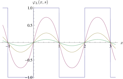
Figure 1: Some plots of the function (4.23) with $l=1$ for $s=0,\frac{1}{10},\frac{1}{2},1$ (from the above).

Note that $\varphi(x,0)$ shows the form of the square wave function, which is set by the boundary condition. When $s=1$, it becomes

$$\varphi_{L}(x,s=1)=\sum_{n=-\infty}^{\infty}(-1)^{n}\tanh(x-nl),$$ (4.24)

which is nothing but a different representation of the Jacobi elliptic function in (4.16).

5 Geometric part

For the geometry part, one finds that $a$ and $b$ behave as

$$a(x,y)=a_{H0}(x)+\cos^{2}y\,a_{H1}(x)+\cos^{4}y\,a_{H2}(x)+\cdots,$$

$$b(x,y)=b_{H0}(x)+\cos^{2}y\,b_{H1}(x)+\cos^{4}y\,b_{H2}(x)+\cdots$$ (5.1)

near horizon region, where $y=\frac{\pi}{2}$ still corresponds to the horizon location. On the other hand, near the boundary at infinity, they should have the expansion

$$a(x,y)=\sin^{2}y\,a_{1}(x)+\sin^{4}y\,a_{2}(x)+\sin^{6}y\,a_{3}(x)+\cdots,$$

$$b(x,y)=b_{0}(x)+\sin^{2}y\,b_{1}(x)+\sin^{4}y\,b_{2}(x)+\cdots,$$ (5.2)

where $a_{0}$ term is not allowed, and $a_{1}$ and $b_{0}$ are related to the extra mass density of black hole induced by the multiple interfaces. The term of order $s^{-1/2}=1/\sin y$ can be added representing the freedom of coordinate transformations. We shall get back to this issue in the analysis of examples below.

The back reaction to the gravity sector is determined by two equations, (3.15) and (3.16). We plug the solution (4.20) into (3.15), getting

$$4\sin^{2}y(\vec{\partial}\varphi)^{2}=4\sin^{2}y\sum_{n_{1},n_{2}}\alpha_{n_{1}}\alpha_{n_{2}}\vec{\partial}\varphi_{0}(x-l_{n_{1}},y)\cdot\vec{\partial}\varphi_{0}(x-l_{n_{2}},y)$$ (5.3)

for the right hand side. It is convenient to split this into the “diagonal” part

$$4\sin^{2}y\sum_{n=-\infty}^{\infty}\alpha^{2}_{n}(\vec{\partial}\varphi_{0}(x-l_{n},y))^{2}$$ (5.4)

and the “off-diagonal” part

$$4\sin^{2}y\sum_{n_{1}<n_{2}}2\alpha_{n_{1}}\alpha_{n_{2}}\vec{\partial}\varphi_{0}(x-l_{n_{1}},y)\cdot\vec{\partial}\varphi_{0}(x-l_{n_{2}},y).$$ (5.5)

The linearity of (3.15) allows us to find its solution by adding the solution with the source term (5.4) and the one with (5.5). Each source term for the diagonal part is the same as that for the black Janus up to the translation in $x$. One may then easily find the solution for the diagonal part

$$a^{\rm diag}(x,y)=b^{\rm diag}(x,y)=\sum_{n=-\infty}^{\infty}\alpha_{n}^{2}\,\Big{[}q_{0}(x-l_{n},y)+C_{n}\frac{\sinh(x-l_{n})}{\sin y}\Big{]},$$ (5.6)

where

$$q_{0}(x,y)=3\,\frac{\sinh x}{\sin y}\,\left(\tan^{-1}\left(\frac{\sinh x}{\sin y}\right)-\frac{\pi}{2}\right)+2+\frac{\sin^{2}y}{\sinh^{2}x+\sin^{2}y}.$$ (5.7)

Later we shall show that the different choices of $C_{n}$ are all related by an appropriate coordinate transformation. Hence we can set $C_{n}=0$ without loss of generality.

5.1 Off-diagonal part

Finding a closed form of the off-diagonal part is rather involved. First step in that direction should be finding a solution of the equation with a term in the off-diagonal source term (5.5). Since one has a translational invariance in $x$ direction and $l>0$ is arbitrary, it suffices to consider the case of $n_{1}=0$ and $n_{2}=1$ with $l_{0}=0$ and $l_{1}=l$. This leads to the equations

$$-2a_{c}(x,y,l)+\sin^{2}y\,\,\vec{\partial}^{2}a_{c}(x,y,l) = \frac{4(\cosh l+XY)}{(1+X^{2})^{3/2}(1+Y^{2})^{3/2}},$$ (5.8)

$$-2\tan y\,\,\partial_{y}\,b_{c}(x,y,l)+\sin^{2}y\,\,\vec{\partial}^{2}b_{c}(x,y,l) = 4a_{c}(x,y;l),$$ (5.9)

where we have introduced

$$X=\frac{\sinh x}{\sin y},\quad Y=\frac{\sinh(x-l)}{\sin y}.$$ (5.10)

Once the solution of the above equations is given, the full off-diaginal part of the solution may be given in the form

$$a^{\rm off}(x,y)=\sum_{n_{1}<n_{2}}2\alpha_{n_{1}}\alpha_{n_{2}}\,a_{c}(x-l_{n_{1}},y,l_{n_{2}}-l_{n_{1}}),$$

$$b^{\rm off}(x,y)=\sum_{n_{1}<n_{2}}2\alpha_{n_{1}}\alpha_{n_{2}}\,b_{c}(x-l_{n_{1}},y,l_{n_{2}}-l_{n_{1}}).$$ (5.11)

We first take the range of $x$ and $y$ as $l<x$ and $0\leq\sin y\leq 1$. Then $X$ and $Y$ can take positive real values. We shall describe below how to extend the solution of this region to $x\leq l$.

Remarkably, it turns out that we can find a solution of this equation by taking the ansatz:

$$a_{c}(x,y,l)=\frac{1}{\sqrt{1+X^{2}}\sqrt{1+Y^{2}}}G(m),\quad b_{c}(x,y,l)=H(m)$$ (5.12)

where

$$m=(\sqrt{1+X^{2}}-X)(\sqrt{1+Y^{2}}-Y).$$ (5.13)

Using this ansatz and regarding $m$ and $XY$ as two independent variables, we may cast the above equation into the form:

$$\Gamma_{2}\,G^{\prime\prime}(m)+\Gamma_{1}\,G^{\prime}(m)+\Gamma_{0}\,G(m)=4(\cosh l+XY)$$ (5.14)

where

$$\Gamma_{2} = \frac{1}{2}(1+m^{2})^{2}+m(1+m^{2})\cosh l+m(1+m^{2}+2m\cosh l)\,XY,$$ (5.15)

$$\Gamma_{1} = \frac{1}{4}{(3+m^{2})(m+m^{-1})}+2\cosh l+\frac{1}{2}(1+3m^{2}+4m\cosh l)\,XY,$$ (5.16)

$$\Gamma_{0} = -\frac{1}{4}{(1+3m^{2})(1+3m^{-2})}-(3m+3m^{-1}+2\cosh l)\,XY.$$ (5.17)

Since we treat $XY$ and $m$ independent, (5.14) implies two ordinary differential equations:

$$4 = (m^{3}+m+2m^{2}\cosh l)G^{\prime\prime}+\frac{1}{2}\Big{(}{3m^{2}+1}-4m\cosh l\Big{)}G^{\prime}$$ (5.18)

$$-(3m+3m^{-1}+2\cosh l)G\,,$$

$$-16\cosh l = \Big{(}2(m^{2}+1)^{2}+4m(m^{2}+1)\cosh l\Big{)}G^{\prime\prime}+(m^{3}+4m+3m^{-1}+8\cosh l)G^{\prime}$$ (5.19)

$$-(3m^{2}+10+3m^{-2})G.$$

We may eliminate the second order derivative term and get the following first order equation:

$$2m(1-m^{2})\left(1+m^{2}+2m\cosh l\right)G^{\prime}(m)+\left(3+2m^{2}+3m^{4}+4m(1+m^{2})\cosh l\right)G(m)$$

$$\ =8m(1+m^{2}+2m\cosh l).$$ (5.20)

Indeed one can check that any solution of this first order equation solves the above two second order equations at the same time. Using the homogeneous solution to this equation,

$$G_{h}(m,\cosh l)=\frac{1}{m^{3/2}}(1-m^{2})\sqrt{1+m^{2}+2m\cosh l},$$ (5.21)

one may easily find the solution

$$G(m) = 4G_{h}(m)\int_{0}^{m}\frac{dx}{(1-x^{2})G_{h}(x)}$$ (5.22)

$$= 4G_{h}(m)\int_{0}^{m}dx\frac{x^{3/2}}{(1-x^{2})^{2}\sqrt{1+x^{2}+2x\cosh l}}\,.$$

Using the identity,

$${x^{3\over 2}\over(1-x^{2})^{2}\sqrt{1+x^{2}+2x\cosh l}} = \left({x^{5\over 2}\over 2(1-x^{2})\sqrt{1+x^{2}+2x\cosh l}}\right)^{\prime}$$ (5.23)

$$\quad-{1\over 4}\left({x\over 1+x^{2}+2x\cosh l}\right)^{3\over 2},$$

the solution can be presented in the form

$$G(m)={\cal G}(m,\cosh l)\equiv 2m-{\cal I}(m,\cosh l)G_{h}(m,\cosh l),$$ (5.24)

where the integral ${\cal I}(x,\cosh l)$ is given by

$${\cal I}(m,\cosh l)=\int_{0}^{m}dx\left({x\over 1+x^{2}+2x\cosh l}\right)^{3\over 2}.$$ (5.25)

Of course one may add the homogeneous part of the solution $C_{G}G_{h}(m)$ to the above with $C_{G}$ being an integration constant. We note that the integral ${\cal I}(m)$ can be evaluated explicitly in terms of the elliptic functions. The details are given in Appendix A.

5.2 Remaining off-diagonal part

Now we turn to the second equation, (5.9) for the metric. Again the linearity of the equation allows us to find the desired solution by summing every solution associated with each term in the right hand side of the equation. With the ansatz in (5.12), (5.9) becomes

$$2m\left(1+m^{2}+2m\cosh l\right)H^{\prime\prime}(m)+\left(5m^{2}-1+4m\cosh l\right)H^{\prime}(m)=8G(m)$$ (5.26)

where we use the general solution

$$G(m)={\cal G}(m)+C_{G}\,G_{h}(m)$$ (5.27)

constructed in the previous section. This equation is essentially first order with respect to $H^{\prime}$. We introduce the homogeneous solution $Q$ given by

$$Q(m)=\frac{m^{\frac{1}{2}}}{(1+m^{2}+2m\cosh l)^{\frac{3}{2}}},$$ (5.28)

Then Eq. (5.26) can be rewritten as

$$\left(\frac{H^{\prime}}{Q}\right)^{\prime}=4\frac{\left(1+m^{2}+2m\cosh l\right)^{\frac{1}{2}}}{m^{\frac{3}{2}}}\,G(m).$$ (5.29)

Now note that the right hand side can be rearranged as

$$\left(\frac{H^{\prime}}{Q}\right)^{\prime}=\left[2\left(\frac{1+m^{2}+2m\cosh l}{m}\right)^{2}\left({\cal I}(m)-C_{G}\right)\right]^{\prime}+6\left(\frac{1+m^{2}+2m\cosh l}{m}\right)^{\frac{1}{2}}.$$ (5.30)

Now integral of this yields

$$\frac{H^{\prime}}{Q}=2\left(\frac{1+m^{2}+2m\cosh l}{m}\right)^{2}\,\,\left({\cal I}(m)-C_{G}\right)+6{\cal M}(m)+8C_{G}\sinh^{2}l$$ (5.31)

where ${\cal M}(m)$ is defined by

$${\cal M}(m,\cosh l)\equiv\int_{0}^{m}dx\left(\frac{1+x^{2}+2x\cosh l}{x}\right)^{1\over 2}$$ (5.32)

and we added an integration constant $8C_{G}\sinh^{2}l$. Now using the identities

$$3{\cal M}(x)+4\sinh^{2}l\,\,\,{\cal I}(x)=\frac{2x^{\frac{1}{2}}}{(1+x^{2}+2x\cosh l)^{\frac{1}{2}}}\,(3+x^{2}+4x\cosh l)$$ (5.33)

$$\frac{(1+x^{2}+2x\cosh l)^{\frac{1}{2}}}{x^{\frac{3}{2}}}-\frac{4x^{\frac{1}{2}}\sinh^{2}l}{(1+x^{2}+2x\cosh l)^{\frac{3}{2}}}=-\left(\frac{2x\,G_{h}(x)}{1+x^{2}+2x\cosh l}\right)^{\prime}$$ (5.34)

one is led to

$$H^{\prime}(m) = 4\left[\frac{2m^{2}}{1+m^{2}+2m\cosh l}+\frac{(1-m^{2})\left(-{\cal I}(m)+C_{G}\right)}{\sqrt{m(1+m^{2}+2m\cosh l)}}\,\,\right]^{\prime}.$$ (5.35)

One more integration provides us with

$$H(m)={4m\over 1+m^{2}+2m\cosh l}G(m)$$ (5.36)

and the homogeneous part of the solution

$$H_{h}(m)=C_{H}\int_{0}^{m}dx\,\frac{x^{\frac{1}{2}}}{(1+x^{2}+2x\cosh l)^{\frac{3}{2}}}+D_{H}$$ (5.37)

can be added to the above in order to obtain a general solution.

5.3 Other types of ansatz

In fact one may try various forms of ansatz that are similar to (5.12). The first alternative is

$$a_{1c}(x,y,l)=\frac{1}{\sqrt{1+X^{2}}\sqrt{1+Y^{2}}}G_{1}(1/m),\quad b_{1c}(x,y,l)=H_{1}(1/m),$$ (5.38)

$$\quad\quad 1/m=(\sqrt{1+X^{2}}+X)(\sqrt{1+Y^{2}}+Y).$$ (5.39)

With this ansatz, one has precisely the same equations whose solution is essentially not different from the previous one given in (5.24). Namely the general solution solution for $G_{1}(1/m)$ is given by

$$G_{1}(1/m)={\cal G}(1/m)+C^{\prime}_{G}G_{h}(1/m).$$ (5.40)

Using the identities

$${\cal G}(1/m)={\cal G}(m)+{\cal I}(\infty)G_{h}(m)\,,\ \ \ \ G_{h}(1/m)=-G_{h}(m),$$ (5.41)

one can show that

$$G_{1}(1/m)={\cal G}(m)+\left({\cal I}(\infty)-C^{\prime}_{G}\right)G_{h}(m).$$ (5.42)

Similar analysis can be done for $H_{1}(1/m)$. Thus no new solution is generated by this ansatz.

The second alternative one may try is the form

$$a_{2c}(x,y,l)=\frac{1}{\sqrt{1+X^{2}}\sqrt{1+Y^{2}}}G_{2}(\bar{m}),\quad b_{2c}(x,y,l)=H_{2}(\bar{m}),$$ (5.43)

$$\quad\quad\bar{m}=(\sqrt{1+X^{2}}-X)(\sqrt{1+Y^{2}}+Y).$$ (5.44)

This ansatz leads to the equations which agrees with (5.14) and (5.26) by the replacement:

$$\bar{m}\rightarrow m\,,\ \ \ XY\rightarrow-XY\,,\ \ \ \cosh l\rightarrow-\cosh l\,,\ \ \ G_{2},H_{2}\rightarrow-G,-H$$ (5.45)

Using this property, the solution can be found as

$$G_{2}(\bar{m})=-{\cal G}(\bar{m},-\cosh l)\,,\ \ \ H_{2}(\bar{m})=-{4\bar{m}\over 1+\bar{m}^{2}-2\bar{m}\cosh l}\,\,{\cal G}(\bar{m},-\cosh l)$$ (5.46)

plus the corresponding homogeneous part which does not play any role in our discussion below. The last alternative one may try is the form

$$a_{3c}(x,y,l)=\frac{1}{\sqrt{1+X^{2}}\sqrt{1+Y^{2}}}G_{3}(1/\bar{m})\,,\ \ \ b_{3c}(x,y,l)=H_{3}(1/\bar{m})$$ (5.47)

$$\quad\quad 1/\bar{m}=(\sqrt{1+X^{2}}+X)(\sqrt{1+Y^{2}}-Y),$$ (5.48)

but the corresponding solution is essentially the same as that from the second alternative ansatz.

Thus the solution can be in general of the form

$$(1-\delta)G(m)+\delta\,G_{2}(\bar{m}),\quad(1-\delta)H(m)+\delta\,H_{2}(\bar{m})$$ (5.49)

and we shall show that $\delta$ has to be zero to satisfy the required boundary conditions. For this purpose, it suffices to consider the limit where $l$ goes to zero. In this limit the cross term should be reduced to the diagonal solution in (5.7) up to the homogeneous part of the solution. Note that

$$\frac{1}{\sqrt{1+X^{2}}\sqrt{1+Y^{2}}}{\cal G}(m,\cosh l)\longrightarrow\ 3X\,\left(\tan^{-1}X-\frac{\pi}{2}\right)+3-\frac{X^{2}}{1+X^{2}}=q_{0}(x.y)$$ (5.50)

and

$$-\frac{1}{\sqrt{1+X^{2}}\sqrt{1+Y^{2}}}{\cal G}(\bar{m},-\cosh l)\longrightarrow\ -{2\over 1+X^{2}}$$ (5.51)

in the limit $l$ goes to zero. Comparing (5.50) with (5.7), we have a precise agreement with each other. Then to satisfy the required boundary conditions in the limit $l\rightarrow 0$, $\delta$ has to be zero since the solution $-{2\over 1+X^{2}}$ by itself does not satisfy the required boundary conditions. (This conclusion does not change even if one includes any possible homogeneous part of solutions.)

Thus the solution for the cross term including the homogeneous part becomes

$$a_{c}(x,y,l) = \frac{1}{\sqrt{1+X^{2}}\sqrt{1+Y^{2}}}\,\Big{(}{\cal G}(m,\cosh l)+C_{G}G_{h}(m,\cosh l)\Big{)},$$ (5.52)

$$b_{c}(x,y,l) = {4m\over 1+m^{2}+2m\cosh l}\,\Big{(}{\cal G}(m,\cosh l)+C_{G}G_{h}(m,\cosh l)\Big{)}.$$ (5.53)

Finally the full off-diagonal part can be constructed in the form (5.11) using the above.

6 Double interfaces

As described before, we consider the boundary condition for the scalar given by

$$\varphi(x,0)=\alpha_{-}\epsilon(x)+\alpha_{+}\epsilon(x-l)=\epsilon(x)-\epsilon(x-l).$$ (6.1)

(In Fig. 2, we depict this boundary condition as well as the one with $\alpha_{-}=\alpha_{+}=1$.)

Figure 2: (a) describes the boundary condition, $\varphi(x,0)$, for $\alpha_{-}=-\alpha_{+}=1$ while (b) for $\alpha_{-}=\alpha_{+}=1$.

The scalar part of the solution has been given in (4.22). The full geometric part of the solution takes the form

$$a(x,y,l)=q_{0}(x,y)+q_{0}(x-l,y)+3\pi Y-2a_{c}^{0}(x,y,l),$$ (6.2)

$$b(x,y,l)=q_{0}(x,y)+q_{0}(x-l,y)+3\pi Y-2b_{c}^{0}(x,y,l),$$ (6.3)

where $a^{0}_{c}(x,y,l)$ and $b^{0}_{c}(x,y,l)$ represents the unit-coefficient cross-term solution given by

$$a^{0}_{c}(x,y,l) = \frac{1}{\sqrt{1+X^{2}}\sqrt{1+Y^{2}}}\,\,\,\Big{(}{\cal G}(m,\cosh l)+{1\over 2}\Delta(l)G_{h}(m,\cosh l)\Big{)},$$ (6.4)

$$b^{0}_{c}(x,y,l) = {4m\over 1+m^{2}+2m\cosh l}\,\,\Big{(}{\cal G}(m,\cosh l)+{1\over 2}\Delta(l)G_{h}(m,\cosh l)\Big{)}.$$ (6.5)

Note that we have added here appropriate homogeneous solutions to make the solution even under the exchange

$$x\ \leftrightarrow\ l-x$$ (6.6)

To see this, we first observe that

$$m\leftrightarrow 1/m\,,\quad\quad X\leftrightarrow-Y$$ (6.7)

under the exchange. Then one finds

$${\cal G}(m)+{1\over 2}\Delta(l)G_{h}(m)$$ (6.8)

is symmetric under the exchange, which one can show using the identity

$${\cal G}(m)+{1\over 2}\Delta(l)\,G_{h}(m)=\frac{1}{2}\Big{(}{\cal G}(m)+{\cal G}(1/m)\Big{)}.$$ (6.9)

Further using the identity

$$q_{0}(x-l,y)+3\pi Y=q_{0}(l-x,y),$$ (6.10)

one finds that the remaining part of the solution is also symmetric under the exchange.

6.1 Shape of the boundary

The change in the shape of the boundary in $(x,y)$ space is of particular interest. Near boundary region, the diagonal and cross terms behave completely differently. Since the solution has the symmetry under the exchange $x\leftrightarrow l-x$, we shall describe the behaviors of the two terms for the regions $l\leq x$ and $0<x<l$ only. Then the remaining region $x\leq 0$ will be given by the reflection symmetry. For the region $0<x<l$ there is no singular term in $q_{0}(x,y)$ and $q_{0}(x-l,y)+3\pi Y$. They behave

$$q_{0}(x,y)=-\frac{2\sin^{4}y}{5\sinh^{4}x}+O(\sin^{6}y),\quad\quad{\rm for}\quad 0\leq x,$$ (6.11)

$$q_{0}(x-l,y)+3\pi Y=-\frac{2\sin^{4}y}{5\sinh^{4}(x-l)}+O(\sin^{6}y),\quad\quad{\rm for}\quad x\leq l.$$ (6.12)

On the other hand, the cross term behaves

$$a_{c}(x,y)=a^{c}_{1}(x)\sin^{2}y+a^{c}_{2}(x)\sin^{4}y+O(\sin^{6}y),$$ (6.14)

$$b_{c}(x,y)=b^{c}_{0}(x)+b^{c}_{1}(x)\sin^{2}y+O(\sin^{4}y)$$ (6.15)

for $0<x<l$. Since there are no boundary terms which show singular behavior as powers of $\sin y$, the boundary of space remains at $y=0$, as illustrated in Fig. 3.

Figure 3: The shape of the boundary in $(x,y)$ space is depicted for $\gamma^{2}=0.1$, $l=1$ and $\alpha_{-}=-\alpha_{+}=1$. The cusps represent the locations of interfaces. We use the convention where the coordinate $y$ grows in the upward direction.

For $l\leq x$, the situation is quite different: $q_{0}(x,y)$ term remains nonsingular. But the terms $3\pi Y$ and $G_{h}(m)$ in both of $a(x,y,l)$ and $b(x,y,l)$ involve the $1/\sin y$ singularity, which implies that the boundary deviates from $y=0$. Let us look at some details of this change of boundary. Basically we would like to show that the singular homogeneous terms are precisely the terms that are required for new metric (including the change of boundary) to be the form of the original BTZ metric without any deformation. To show this, we begin with

$$ds^{2}=\frac{1}{\sin^{2}y}\left[\frac{dx^{2}+dy^{2}}{1+\frac{\gamma^{2}}{4}a_{h}(x,y)+O(\gamma^{4})}+\frac{\cos^{2}y\,\,d\tau^{2}}{1+\frac{\gamma^{2}}{4}b_{h}(x,y)+O(\gamma^{4})}\right]$$ (6.16)

where $a_{h}$ and $b_{h}$ denote the homogeneous part of the solution. Then by the coordinate transformation,

$$y^{\prime}=y+\frac{\gamma^{2}}{4}\,\cos y\,\,{\cal A}_{h}(x,y)+O(\gamma^{4}),$$

$$x^{\prime}=x+\frac{\gamma^{2}}{4}\cosh x\,{\cal B}_{h}(x,y)+O(\gamma^{4}),$$ (6.17)

one can bring the metric into the original BTZ form

$$ds^{2}=\frac{1}{\sin^{2}y^{\prime}}\left[d{x^{\prime}}^{2}+d{y^{\prime}}^{2}+\cos^{2}y^{\prime}\,d\tau^{2}\right].$$ (6.18)

Comparing $g^{\prime}_{\tau\tau}$ and $g_{\tau\tau}$ components, one finds

$${\cal A}_{h}(x,y)=\frac{1}{2}b_{h}(x,y)\sin y$$ (6.19)

together with the conditions

$$\frac{1}{\cosh x}\partial_{x}{\cal A}_{h}+\frac{1}{\cos y}\partial_{y}{\cal B}_{h}=0,$$ (6.20)

$$\frac{1}{\cos y}\partial_{y}{\cal A}_{h}-{\cal A}_{h}\sin y-{\cal A}_{h}\cos^{2}y=-\frac{1}{2}a_{h},$$ (6.21)

$$\frac{1}{\cosh x}\partial_{x}{\cal B}_{h}+{\cal B}_{h}\sinh x-{\cal A}_{h}\cos^{2}y=-\frac{1}{2}a_{h}.$$ (6.22)

Combining these equations and eliminating ${\cal A}_{h}$ and ${\cal B}_{h}$, one finds our original equations (3.15)-(3.16) without the source term,

$$2a_{h}-\sin^{2}y\,\,\vec{\partial}^{2}a_{h}=0,$$ (6.23)

$$2\tan y\,\partial_{y}b_{h}-\sin^{2}y\,\,\vec{\partial}^{2}b_{h}+4a_{h}=0,$$ (6.24)

together with the relation

$$a_{h}=b_{h}\sin^{2}y-\sin y\cos y\partial_{x}b_{h}.$$ (6.25)

Showing this for the homogeneous part of the cross term solution is not that straightforward and its proof will be relegated to Appendix B. For the diagonal part, the above relation can be checked immediately for homogeneous solution $a^{\rm diag}_{h}(x,y)=b^{\rm diag}_{h}(x,y)=\frac{\sinh x}{\sin y}$.

Figure 4: The shape of the boundary in $(x,y)$ space is depicted for $\gamma^{2}=0.1$, $l=1$ and $\alpha_{-}=\alpha_{+}=1$. The change of the boundary is in the opposite direction compared to the configuration in Fig. 3.

Thus this proves the existence of the function ${\cal A}_{h}$ and the corresponding coordinate transformation. The resulting form of the coordinate transformation for $y^{\prime}$ reads explicitly

$$y^{\prime}=y+\frac{\gamma^{2}}{8}\left[3\pi\sinh(x-l)\cos y-4\Delta(l)\frac{\frac{1}{m}-m}{\sqrt{m+\frac{1}{m}+2\cosh l}}\sin y\cos y\right]+O(\gamma^{4})$$ (6.26)

for $x\geq l$. The boundary defined by $y^{\prime}=0$ is determined by the equation

$$\sin y=\frac{\gamma^{2}}{8}\left[4\Delta(l)\frac{\frac{1}{m}-m}{\sqrt{m+\frac{1}{m}+2\cosh l}}\sin y-3\pi\sinh(x-l)\right]+O(\gamma^{4}).$$ (6.27)

For general grounds, one expects that the curve defined by (6.27) can be solved in the form

$$\sin y=\gamma^{2}g(x)+O(\gamma^{4})$$ (6.28)

with some $O(1)$ function $g(x)$. Consider the case where

$$X=\frac{\sinh x}{\sin y}=\frac{\sinh x}{g(x)}\gamma^{-2}+O(\gamma^{0})\gg 1,$$

$$Y=\frac{\sinh(x-l)}{\sin y}=\frac{\sinh(x-l)}{g(x)}\gamma^{-2}+O(\gamma^{0})\gg 1.$$ (6.29)

Assuming these, the curve (6.27) is solved by

$$\sin y={\gamma^{2}}\left(\Delta(l)\sqrt{\sinh x\sinh(x-l)}-\frac{3\pi}{8}\sinh(x-l)\right)+O(\gamma^{4})$$ (6.30)

and thus

$$g(x)=\Delta(l)\sqrt{\sinh x\sinh(x-l)}-\frac{3\pi}{8}\sinh(x-l).$$ (6.31)

Using this, one finds that our original conditions in (6.29) are met if

$$\sqrt{x-l}\ \gg\ \gamma^{2}\Delta(l)\sinh l.$$ (6.32)

For $x/l\gg 1$, the boundary trajectory is further simplified as

$$\sin y={\gamma^{2}}\left(\Delta(l)\,\,e^{\frac{l}{2}}-\frac{3\pi}{8}\right)\sinh(x-l)+O(\gamma^{4}).$$ (6.33)

For the region where the condition (6.32) is violated, one finds the solution of (6.27) is

$$\sin y=O(\gamma^{4}).$$ (6.34)

Determining its precise functional form lies beyond the scope of our approximation since it requires the knowledge of $O(\gamma^{4})$ corrections to the geometry. The full shape of the boundary including a solution of (6.27) for $x>l$ is depicted in Fig. 3. This may be compared with the boundary shape of the double interface system with $\alpha_{-}=\alpha_{+}=1$, which is depicted in Fig. 4

6.2 Casimir energy and pressure

In this subsection, we shall construct the Fefferman-Graham metric to determine the boundary stress energy tensor. In order to use the prescription developed in Ref. [21], we introduce the metric in the following Fefferman-Graham form,

$$ds^{2}={d\chi^{2}\over\chi^{2}}+{1\over\chi^{2}}g_{\mu\nu}(q,\chi)dq^{\mu}dq^{\nu}$$ (6.35)

where $q^{\mu}$ ($\mu=0,\,1$) denote the boundary coordinates and $\chi=0$ corresponds to the location of the boundary. In general one may expand $g_{\mu\nu}$ by

$$g_{\mu\nu}(q,\chi)=g^{(0)}_{\mu\nu}(q)+\chi^{2}g^{(2)}_{\mu\nu}(q)+\cdots$$ (6.36)

where $g^{(0)}_{\mu\nu}$ is the metric for the boundary system. In three dimensions, the boundary stress energy tensor is then given by [21]

$$T_{\mu\nu}(q)={1\over 8\pi G}\left[g^{(2)}_{\mu\nu}(q)-g^{(0)}_{\mu\nu}(q)\,g^{(2)}_{\alpha\beta}(q)g^{(0)\alpha\beta}(q)\right]+\tau_{\mu\nu}(q)$$ (6.37)

where $\tau_{\mu\nu}(q)$ is the scalar contribution for the stress energy tensor given by

$$\tau_{\mu\nu}(q)={1\over 8\pi G}\Big{[}\partial_{\mu}\phi_{B}\partial_{\nu}\phi_{B}-{g^{(0)}_{\mu\nu}\over 2}\,g^{(0)\alpha\beta}\partial_{\alpha}\phi_{B}\partial_{\beta}\phi_{B}\Big{]}$$ (6.38)

with $\phi_{B}$ denoting the boundary value of the scalar field. For our case, the boundary metric is given by

$$g^{(0)}_{\mu\nu}={\rm diag}(-1,1)=\eta_{\mu\nu}$$ (6.39)

since the boundary system is defined in the flat Minkowski space in two dimensions and the scalar contribution to the stress energy tensor vanishes since the scalar field is constant except $x=0,\,\,l$. Let us first bring the metric in (3.21) to the form

$$ds^{2}={dp^{2}\over\sin^{2}p}+{dq_{1}^{2}\over\sin^{2}p}\Big{(}1-{\gamma^{2}\over 4}D_{1}(x,y)\,\Big{)}-{dq_{0}^{2}}\cot^{2}p\,\Big{(}1-{\gamma^{2}\over 4}D_{2}(x,y)\,\Big{)}$$ (6.40)

where $q_{0}=-i\tau$. Introducing ${\cal X}_{FG}(x,y)$ and ${\cal Y}_{FG}(x,y)$ by

$$q_{1}(x,y)=x-{{\gamma^{2}\over 8}}{\cal X}_{FG}(x,y)+O(\gamma^{4}),\qquad p(x,y)=y-{{\gamma^{2}\over 8}}{\cal Y}_{FG}(x,y)+O(\gamma^{4})$$ (6.41)

and comparing the two forms of the metric to the $O(\gamma^{2})$, one finds the differential equations

$$\partial_{y}{\cal Y}_{FG}-{\cal Y}_{FG}\,\cot y=a(x,y),\quad\partial_{x}{\cal Y}_{FG}+\partial_{y}{\cal X}_{FG}=0$$ (6.42)

with

$$D_{1}(x,y)=a(x,y)-\partial_{x}{\cal X}_{FG}+{\cal Y}_{FG}\,\cot y,$$

$$D_{2}(x,y)=b(x,y)+{{\cal Y}_{FG}\over\sin y\cos y}.$$ (6.43)

The boundary conditions $D_{1}(x,0)=D_{2}(x,0)=0$ are required to have the standard form of the boundary metric $\eta_{\mu\nu}$.

For the regions $x\geq l$ and $x\leq 0$, after change of the coordinate transformation in (6.17), the transformed solutions behave

$$a^{\prime}(x^{\prime},y^{\prime})=O(\sin^{4}y^{\prime})\,,\quad\quad\quad b^{\prime}(x^{\prime},y^{\prime})=O(\sin^{4}y^{\prime})$$ (6.44)

and one can show that there is no stress-energy contribution except that of the original, undeformed BTZ black hole.

Let us turn our attention to the region between the interfaces, $0\leq x\leq l$. For the diagonal part, the asymptotic behaviors in (6.44) still hold in this region and, thus, it does not contribute to the stress tensor. For the case of the cross-term, the situation is different and one expects an extra contribution to the stress tensor, which leads to a nonvanishing Casimir energy. We shall analyze the details by constructing the corresponding Fefferman-Graham metric in the near-boundary region.

We note that the solution has the expansion

$$a(x,y)=a_{1}(x)\sin^{2}y+a_{2}(x)\sin^{4}y+O(\sin^{6}y),$$ (6.45)

$$b(x,y)=b_{0}(x)+b_{1}(x)\sin^{2}y+O(\sin^{4}y)$$ (6.46)

in the region between the interface. Then the corresponding solution of satisfying (6.42) the boundary condition $D_{1}(x,0)=D_{2}(x,0)=0$ is given by

$${\cal X}_{FG}=-\int dx\,b_{0}(x)+b^{\prime}_{0}(x)(1-\cos y)+O(\sin^{4}y),$$ (6.47)

$${\cal Y}_{FG}=\left[-b_{0}(x)+a_{1}(x)(1-\cos y)+O(\sin^{4}y)\,\,\right]\sin y,$$ (6.48)

where the prime denotes the derivative with respect to the argument. Then $D_{2}(x,y)$ and $D_{2}(x,y)$ can be expanded as

$$D_{1}(x,y)=-\frac{b^{\prime\prime}_{0}-b_{0}-3a_{1}}{2}\sin^{2}y+O(\sin^{4}y),$$ (6.49)

$$D_{2}(x,y)=\frac{b^{\prime\prime}_{0}-b_{0}-3a_{1}}{2}\sin^{2}y+O(\sin^{4}y),$$ (6.50)

where we have the relation

$$b_{1}(x)=-\frac{4a_{1}-b^{\prime\prime}_{0}}{2}$$ (6.51)

which holds for any nonsingular solutions of the geometric part.

Now explicitly,

$$a_{1}(x)=-2\frac{1}{\sinh x\sinh(l-x)}\left({\cal G}(m_{0})+{1\over 2}\Delta(l)G_{h}(m_{0})\right),$$ (6.52)

$$b_{0}(x)=-2\frac{4}{m_{0}+\frac{1}{m_{0}}+2\cosh l}\left({\cal G}(m_{0},\cosh l)+{1\over 2}\Delta(l)G_{h}(m_{0})\right),$$ (6.53)

where

$$m_{0}=\frac{\sinh(l-x)}{\sinh x}.$$ (6.54)

A crucial simplification comes from the relation

$$b^{\prime\prime}_{0}-b_{0}-3a_{1}=(-2)\frac{8}{\sinh^{2}l},$$ (6.55)

where the extra factor $(-2)$ reflects the fact that the cross term for the current case comes with extra factor $(-2)$. Thus finally,

$$D_{1}(x,y)=\frac{8}{\sinh^{2}l}\sin^{2}y+O(\sin^{4}y),$$ (6.56)

$$D_{2}(x,y)=-\frac{8}{\sinh^{2}l}\sin^{2}y+O(\sin^{4}y).$$ (6.57)

The rest is straightforward. Noting

$$\chi=2\tan{q\over 2}$$ (6.58)

one finds

$$g_{\mu\nu}^{(2)}=\left({1\over 2}-\frac{2}{\sinh^{2}l}\Theta(x)\Theta(l-x)\gamma^{2}\right){\rm diag}(+1,+1)+O(\gamma^{4})$$ (6.59)

with the step function $\Theta(x)=\frac{1+\epsilon(x)}{2}$. Therefore, one has

$$T_{\mu\nu}={1\over 16\pi G}\left(1-\frac{4\gamma^{2}}{\sinh^{2}l}\Theta(x)\Theta(l-x)\right){\rm diag}(+1,+1)+O(\gamma^{4}).$$ (6.60)

Finally recovering the temperature dependence by the scaling transformation, we have

$$T_{\mu\nu}=\frac{\pi^{2}\,T^{2}-\frac{4\pi^{2}T^{2}\gamma^{2}}{\sinh^{2}2\pi Tl}\Theta(x)\Theta(l-x)}{4\pi G}{\rm diag}(+1,+1)+O(\gamma^{4})$$ (6.61)

which clearly shows the effect of the Casimir energy between the interfaces. The Casimir energy density and pressure are respectively given by

$${\cal E}_{C}=-\frac{2c}{3}\frac{\pi T^{2}}{\sinh^{2}2\pi Tl}\Theta(x)\Theta(l-x)\,\gamma^{2}+O(\gamma^{4}),$$ (6.62)

$$p_{C}=-\frac{2c}{3}\frac{\pi T^{2}}{\sinh^{2}2\pi Tl}\,\gamma^{2}+O(\gamma^{4}),$$ (6.63)

and the pressure is acting on the interfaces. The Casimir energy contribution is negative and the corresponding pressure is negative (attractive). For the general case of double interfaces, the factor $-2$ in the above expression is replaced by $2\alpha_{+}\alpha_{-}$. For the double interfaces with $\alpha_{+}\alpha_{-}>0$, the Casimir energy contribution becomes now positive reflecting the repulsive nature of the same-signature interfaces. For the general double interfaces, the energy becomes

$$E=\frac{c}{6}\left[\pi T^{2}L+\frac{2\pi T^{2}l}{\sinh^{2}2\pi Tl}(2\alpha_{+}\alpha_{-})\gamma^{2}+O(\gamma^{4})\right]$$ (6.64)

where the full size $L$ of the system should be taken to be large to avoid any finite size effect.

6.3 Geometric entropy of the double interfaces

In this section we shall compute the entropy of the double-interface system from the geometric side. In the later section, we shall compare the results with those from the direct field-theory computation and show that they agree with each other.

The interface contribution from the diagonal terms has been computed in [15] to all order in $\gamma$. For each of unit-coefficient diagonal term, the entropy correction reads [15]

$$\delta S^{0}_{\rm diag}=\frac{1}{4G}\gamma^{2}+O(\gamma^{4}).$$ (6.65)

Therefore, the total diagonal contribution for the double interfaces reads

$$\delta S^{\rm diag}=\frac{1}{4G}(\alpha_{+}^{2}+\alpha^{2}_{-})\gamma^{2}+O(\gamma^{4})=\frac{1}{2G}\gamma^{2}+O(\gamma^{4})$$ (6.66)

with $\alpha_{-}=-\alpha_{+}=1$.

Let us compute here the entropy correction due to the off-diagonal terms. For this we put the boundary system in a box with a size $L=2w_{0}$ and consider the region $-w_{0}+\frac{l}{2}\leq q_{1}\leq w_{0}+\frac{l}{2}$ where $q_{1}$ is the Fefferman-Graham coordinate defined in (6.41). To avoid any finite size effect, we shall assume $w_{0}\gg l$ and $w_{0}\gg 1$ and consider one half of the box specified by $\frac{l}{2}\leq q_{1}\leq w_{0}+\frac{l}{2}$ utilizing the symmetry of the solution we are considering.

First let us translate the boundary coordinate $q_{1}$ to our original coordinate $x$. As identified in (6.41), (6.44) and (6.47), one has

$$q_{1}=x+\frac{\gamma^{2}}{8}\Theta(x)\Theta(l-x)\int^{x}_{\frac{l}{2}}dx^{\prime}b_{0}(x^{\prime})+O(\gamma^{4})$$ (6.67)

which is along the boundary we identified in the previous section. For $x=\frac{l}{2}$, we let $q_{1}=\frac{l}{2}$ by adjusting the integration constant. Let $x_{B}$ be the $x$-coordinate value corresponding to $q_{1}=w_{0}+\frac{l}{2}$. The from the above relation, one finds

$$x_{B}=w_{0}+\frac{l}{2}+\delta x_{B}$$ (6.68)

with

$$\delta x_{B}=-\frac{\gamma^{2}}{8}\int^{l}_{\frac{l}{2}}dx^{\prime}b_{0}(x^{\prime})+O(\gamma^{4}).$$ (6.69)

We evaluate this expression for the unit-coefficient cross term

$$b^{c}_{0}(x)=\frac{4}{m_{0}+\frac{1}{m_{0}}+2\cosh l}\left({\cal G}(m_{0},\cosh l)+{1\over 2}\Delta(l)G_{h}(m_{0})\right)$$ (6.70)

where $m_{0}(x)$ is given in (6.54) and we strip off the factor $2\alpha_{+}\alpha_{-}$. Of course, we shall recover this factor in order to obtain the full contribution. The integral can be straightforwardly evaluated, which leads to

$$\delta x_{B}=-\frac{\gamma^{2}}{2}\left(\coth l-\frac{l}{\sinh^{2}l}\right)+O(\gamma^{4}).$$ (6.71)

The details of computation are relegated to Appendix C. We illustrate the relation between $x$ and $q_{1}$ coordinates along the boundary in Fig. 5.

Figure 5: The relation between $x$ and $q_{1}$ coordinate along the boundary is depicted for the double interfaces with the coefficients $\alpha_{-}=-\alpha_{+}=1$. The thick line represents the horizon located at $y=\pi/2$. The dotted lines represent the trajectories determined by the boundary-horizon map.

Next we turn to the problem of the boundary-horizon map to find the horizon point corresponding to $x=x_{B}$. (For $x=\frac{l}{2}$, we choose $x_{H}=\frac{l}{2}$.) We shall use the method [15] based on the conserved current. (Alternatively one may use the method based on the lightlike geodesics orthogonal to the boundary [22], which leads to the same result in the large size limit.) The condition reads

$$dx^{a}\epsilon_{abc}\nabla^{b}\xi^{c}=0$$ (6.72)

where $\xi^{a}$ is the time translation Killing vector. This leads to

$${dx\over dy}={g_{yy}\,\partial_{x}g_{tt}\over g_{xx}\,\partial_{y}g_{tt}}={\gamma^{2}\over 8}\sin y\cos y\,\partial_{x}b(x,y)+O(\gamma^{4})\,.$$ (6.73)

Note that

$$b_{c}(x,y)=2\Delta(l)\frac{e^{x-\frac{l}{2}}}{\sin y}+O(e^{-x})$$ (6.74)

for $x\gg l$ and $x\gg 1$. The above equation is solved by

$$x(y)=x_{B}+\frac{\gamma^{2}}{4}\left[\Delta(l)\sin y\,e^{w_{0}}+O(e^{-w_{0}})\right]+O(\gamma^{4})$$ (6.75)

which describes the map from the boundary point $x=x_{B}$ to the corresponding horizon point. Then at the horizon, the corresponding coordinate $x_{H}$ is given by

$$x_{H}=w_{0}+\frac{l}{2}+\delta x_{B}+\delta x_{H}$$ (6.76)

with

$$\delta x_{H}=\frac{\gamma^{2}}{4}\left[\Delta(l)e^{w_{0}}+O(e^{-w_{0}})\right].$$ (6.77)

The horizon length for the entropy then becomes

$$L_{H}/2 = \int^{x_{H}}_{\frac{l}{2}}dx\Big{(}1-{\gamma^{2}\over 8}a(x,{\frac{\pi}{2}})\Big{)}+O(\gamma^{4})\,$$ (6.78)

$$= (w_{0}+\delta x_{B}+\delta x_{H})-{\gamma^{2}\over 8}\int^{w_{0}+\frac{l}{2}}_{\frac{l}{2}}dx\,a(x,\frac{\pi}{2})+O(\gamma^{4}).$$

The integral can be evaluated as

$$\int^{w_{0}+\frac{l}{2}}_{\frac{l}{2}}dx\,a_{c}(x,{\pi/2})=-4+2\sqrt{2\cosh 2w_{0}+2\cosh l}\left(\Delta(l)-2{\cal I}(e^{-2w_{0}},\cosh l)\right)$$

$$\quad\quad\quad=-4+2e^{w_{0}}\Delta(l)+O(e^{-w_{0}})$$ (6.79)

Thus the length correction due to the unit-coefficient cross term becomes

$$\delta_{c}L_{H}=\gamma^{2}\left[1-\Big{(}\coth l-\frac{l}{\sinh^{2}l}\Big{)}\right]+O(\gamma^{4})$$ (6.80)

in the large $L$ limit. Therefore, the total change of the entropy for the two interfaces is given by

$$\delta S={1\over 4G}(L_{H}-L)={1\over 4G}\left[(\alpha_{+}+\alpha_{-})^{2}-2\alpha_{+}\alpha_{-}\Big{(}\coth l-\frac{l}{\sinh^{2}l}\Big{)}\right]\gamma^{2}+O(\gamma^{4})$$ (6.81)

where we have added the diagonal contribution (6.66).

Figure 6: The entropy of the cross term contribution is depicted for $\alpha_{-}=\alpha_{+}=1$, $c=3$, and $\gamma^{2}=1$. It shows that this contribution of entropy vanishes for the large $Tl$ limit.

Recovering the temperature dependence, one finds

$$S=S_{0}+\delta S=S_{0}+\frac{c}{6}\left[(\alpha_{+}+\alpha_{-})^{2}-2\alpha_{+}\alpha_{-}\Big{(}\coth 2\pi Tl-\frac{2\pi Tl}{\sinh^{2}2\pi Tl}\Big{)}\right]\gamma^{2}+O(\gamma^{4})$$ (6.82)

where $S_{0}$ denotes the undeformed BTZ entropy

$$S_{0}=\frac{c}{3}\pi TL.$$ (6.83)

When $\alpha_{-}=-\alpha_{+}=1$, the entropy correction

$$\delta S=\frac{c}{3}\Big{(}\coth 2\pi Tl-\frac{2\pi Tl}{\sinh^{2}2\pi Tl}\Big{)}\gamma^{2}+O(\gamma^{4})$$ (6.84)

comes from the thermodynamic effect related to the Casimir energy. As $lT\rightarrow 0$, the two interfaces join together and become a single interface with an interface coefficient $\alpha_{+}+\alpha_{-}$. Indeed the entropy correction approaches that of the single interface:

$$\delta S\ \rightarrow\ \frac{c}{6}(\alpha_{+}+\alpha_{-})^{2}\gamma^{2}+O(\gamma^{4}).$$ (6.85)

On the other hand, in the limit where $LT$ becomes infinity, one expects that the two interfaces become independent with each other. The corresponding entropy correction becomes that for the two independent interfaces,

$$\delta S\ \rightarrow\ \frac{c}{6}(\alpha^{2}_{+}+\alpha^{2}_{-})\gamma^{2}+O(\gamma^{4})$$ (6.86)

The behavior of the cross-term entropy correction (as a function of $LT$), for $\alpha_{-}=-\alpha_{+}=1$ and $c=3$, is illustrated in Fig. 6. It clearly shows that the contribution from the cross-term vanishes in the large separation limit of the interface distance.

7 Check of the correspondence

As discussed previously in [13], the corresponding field-theory dual to the Janus deformation is defined by the Lagrangian density

$${\cal L}(t,x)={\cal L}_{0}(t,x)\,e^{-\phi_{B}(x)}$$ (7.1)

where ${\cal L}_{0}$ is the Lagrange density for the original, undeformed CFT and $\phi_{B}$ denotes the boundary value of the bulk scalar field $\phi(x)$ which is dual to the Lagrange density operator. For the deformation of the current problem,

$${\cal L}(t,x)={\cal L}_{0}(t,x)\,\left[1-\gamma\sum_{n}\alpha_{n}\epsilon(x-l_{n})+O(\gamma^{2})\right]$$ (7.2)

where the boundary condition (4.21) is used. We shall consider the finite-temperature field theory which is dual to our deformed black hole geometry constructed in the above.

The free energy,

$$F=-\frac{1}{\beta}\ln{\rm tr}\,e^{-\beta H}$$ (7.3)

can be computed perturbatively as a power series in $\gamma$ using the so-called conformal perturbation theory. Namely,

$${\rm tr}\,e^{-\beta H}$$

$$={\rm tr}\,e^{-\beta H_{0}}\left[1-\frac{1}{2}\int^{\beta}_{0}\!d\tau\int^{\beta}_{0}\!d\tau^{\prime}\int^{\infty}_{-\infty}dx\int^{\infty}_{-\infty}dx^{\prime}\langle\delta{\cal L}(-i\tau,x)\delta{\cal L}(-i\tau^{\prime},x^{\prime})\rangle+O(\gamma^{4})\right]$$ (7.4)

where we have used the fact that

$$\langle{\cal L}_{0}(-i\tau,x)\rangle=0.$$ (7.5)

The expectation value is defined with respect to the undeformed (finite-temperature) CFT in the regime where the gravity and the CFT correspondence is valid. See [13] for the details of the conditions for the gravity approximation. The free energy can be expanded as

$$F=F_{0}+\gamma^{2}F_{2}+O(\gamma^{4})$$ (7.6)

where $F_{0}$ is the undeformed BTZ free energy given by

$$F_{0}=-\frac{c}{6}\pi T^{2}L.$$ (7.7)

Using the two-point function [14] given by

$$\langle{\cal L}(-i\tau,x){\cal L}(-i\tau^{\prime},x^{\prime})\rangle=\frac{1}{16\pi^{2}G}\frac{(2\pi T)^{4}}{\big{[}\cos(\frac{2\pi(\tau-\tau^{\prime})}{\beta})-\cosh(\frac{2\pi(x-x^{\prime})}{\beta})-i\epsilon\big{]}^{2}}$$ (7.8)

and performing the $\tau$ and $\tau^{\prime}$ integrals, one finds $F_{2}$ is given by

$$F_{2}=-\frac{T}{8G}\sum_{n,m}\alpha_{n}\alpha_{m}\int_{-\infty}^{\infty}dx\epsilon(x-2\pi Tl_{n})\int^{\infty}_{-\infty}dx^{\prime}\epsilon(x^{\prime}-2\pi Tl_{m})\,h(x-x^{\prime})$$ (7.9)

where we rescaled $x$ and $x^{\prime}$ by the factor $2\pi T$ and $h(x)$ is given by

$$h(x)=\frac{\cosh(x)+q^{2}}{\big{(}(\cosh(x)+q^{2}\big{)}^{2}-1)^{3/2}}$$ (7.10)

with $q^{2}=i\epsilon$. (The above expression is for the case of infinite-sized box and has to be regulated appropriately by putting the system in a box with a finite size $L$.) For the further evaluation, let us first consider the unit-coefficient cross-term

$$F^{c}_{2}=-\frac{T}{8G}\int_{-\infty}^{\infty}dx\epsilon(x)\int^{\infty}_{-\infty}dx^{\prime}\epsilon(x^{\prime}-2\pi Tl)\,h(x-x^{\prime}).$$ (7.11)

Noting $h(x)=h(-x)$, the above integral is rearranged as

$$F_{2}^{c} = -\frac{T}{8G}\int_{0}^{\infty}dx\int^{\infty}_{-\infty}dx^{\prime}\left(\epsilon(x^{\prime}-2\pi Tl)+\epsilon(x^{\prime}+2\pi Tl)\right)h(x-x^{\prime})$$ (7.12)

$$= -\frac{T}{4G}\int_{0}^{\infty}dx\int^{\infty}_{2\pi Tl}dx^{\prime}\left(h(x-x^{\prime})-h(x+x^{\prime})\right)$$

$$= -\frac{T}{2G}\left[W_{1}(\infty)-W_{2}(2\pi Tl)\right]$$

where

$$W_{1}(w) = \frac{1}{2}\int_{0}^{w}dx\int^{\infty}_{0}dx^{\prime}\left(h(x-x^{\prime})-h(x+x^{\prime})\right)$$ (7.13)

$$= \int_{0}^{w}dx\int^{x}_{0}dx^{\prime}\,h(x^{\prime})$$

and

$$W_{2}(w) = \frac{1}{2}\int_{0}^{\infty}dx\int^{w}_{0}dx^{\prime}\left(h(x-x^{\prime})-h(x+x^{\prime})\right)$$ (7.14)

$$= \int_{0}^{w}dx^{\prime}\int^{x^{\prime}}_{0}dx\,h(x).$$

For the last equality in the above, we have interchanged the order of integrations on $x$ and $x^{\prime}$. $W_{2}(2\pi Tl)$ does not require any regularization related to the box size of the system. On the other hand, $W_{1}(\infty)$ requires a regularization and we shall change the range of integral $(-\infty,\infty)$ to $[-\pi TL,\pi TL]$ leading to the regularized expression $W_{1}(\pi TL)$. Later we shall take the large $TL$ limit to avoid any finite size effect related to the size of the box. Note that $W_{1}(w)=W_{2}(w)=W(w)$. The integral $W(w)$ is found in [15] and the result reads

$$W(w)=\frac{w}{2q^{2}}-\frac{1}{\sqrt{2}\,q}+\frac{1}{2}\coth w+O(q^{2})$$ (7.15)

and, for the regularization with respect to $q^{2}(=i\epsilon)$, we shall keep only the finite part, i.e. $\frac{1}{2}\coth w$. Therefore,

$$F_{2}^{\rm cross}=-\frac{T}{4G}\big{(}1-\coth 2\pi Tl\big{)}$$ (7.16)

where we take the large $TL$ limit ignoring the finite size effect related to the box size.

For the case of a unit-coefficient diagonal term, one can follow the same procedure leading to the result

$$F_{2}^{\rm diag}=-\frac{T}{4G}.$$ (7.17)

Therefore, for the general double interface, one is led to

$$F=-\frac{c}{6}\left[\pi T^{2}L+T\Big{(}(\alpha_{+}+\alpha_{-})^{2}-2\alpha_{+}\alpha_{-}\coth 2\pi Tl\Big{)}\gamma^{2}+O(\gamma^{4}).\right]$$ (7.18)

Using the standard thermodynamic relations,

$$S=-\frac{\partial F}{\partial T}\,,\ \ \ E=F-TS$$ (7.19)

one finds the precise agreement with those from geometric side given in (6.64)and (6.81). One can check the first law

$$TdS=dE+p_{L}dL+p_{l}dl$$ (7.20)

where

$$p_{L}=-\frac{\partial F}{\partial L}=\frac{c}{6}\pi T^{2},\quad p_{l}=-\frac{\partial F}{\partial l}=\alpha_{+}\alpha_{-}\,\frac{c}{3}\frac{2\pi T^{2}}{\sinh^{2}2\pi Tl}\gamma^{2}+O(\gamma^{4})$$ (7.21)

One can check that $p_{l}$ agrees with $p_{c}$ in (6.63) from the geometric side with $\alpha_{+}\alpha_{-}=-1$. Of course $p_{L}$ is in agreement with that from the stree energy tensor in (6.61).

8 General interfaces and the lattice

Until now, we have discussed the detailed properties of the double interface configurations. Extending this analysis to the general interface system is rather straightforward. In this section, we shall describe the boundary shape and the thermodynamic properties of the general interface system. We shall also comment on the properties of the interface lattice briefly.

The solution for the general interface configuration is constructed in (4.21), (4.20), (5.6) and (5.11). Finding the boundary shape for a given interface solution is rather involved. The boundary shape in a particular coordinate system is dependent on the choice of the homogeneous terms though the geometry itself including its boundary should be independent of this choice. This is because different choices of homogeneous solutions are all related by coordinate transformations, as was verified in the previous section. This implies that the shape of the boundary in one coordinate system is affected by the choice of the homogeneous terms. For the homogeneous term $X=\frac{\sinh x}{\sin y}$ that is related to the diagonal solution $q_{0}(x)$, the part of coordinate transformation in (6.17) takes the form

$$y^{\prime}=y+\frac{\gamma^{2}}{8}\cos y\sinh x+O(\gamma^{4}).$$ (8.1)

The trajectory of $y^{\prime}=0$ is described by

$$\sin y=-\frac{\gamma^{2}}{8}\sinh x+O(\gamma^{4}).$$ (8.2)

This is illustrated in Fig. 7 for $\gamma^{2}=0.01$ and $l=1$.

Figure 7: The trajectory $y^{\prime}=0$ is depicted in $(x,y)$ space for the coordinate transformation in relation with the homogeneous solution $X=\frac{\sinh x}{\sin y}$. We take $l=1$ and $\gamma^{2}=0.01$.

It is rather clear that the coordinate transformation is highly nonlinear, which means that any particular trajectory, e.g. $y^{\prime}=0$, has different-looking shapes depending the choices of coordinate system. Similarly for the homogeneous term $G_{h}(x,y,\cosh l)$ related to the cross-term part of the solution, the trajectory $y^{\prime}=0$ has an even complicated shape in the $(x,y)$ coordinate system. Using (6.17), one can identify the trajectory $y^{\prime}=0$ as

$$\sin y=\frac{\gamma^{2}}{8}\left[\Theta(-x)\sqrt{\sinh(-x)\sinh(l-x)}-\Theta(x-l)\sqrt{\sinh x\sinh(x-l)}\,\right]+O(\gamma^{4}).$$ (8.3)

As we see in Fig. 8, the trajectory $y^{\prime}=0$ in the $(x,y)$ plane reflects the highly nonlinear nature of the coordinate transformation. Hence depending on the choice of homogeneous terms, the shapes of the boundary in the $(x,y)$ plane have to change rather drastically and one cannot expect any kinds of shape invariance of under the coordinate transformations.

Figure 8: The trajectory $y^{\prime}=0$ is depicted in $(x,y)$ space for the coordinate transformation in relation with the homogeneous solution $G_{h}(m)$. We take $l=1$ and $\gamma^{2}=0.01$.

Having this complication in mind, with a specific choice of the homogeneous terms, one can in general find the boundary shape of the geometry for the general interface system. For the cases of double interfaces, we have illustrated these boundary shapes in Figs. 3 and 4. As a further illustration, here we consider a three interface configuration with a boundary condition of the scalar field,

$$\varphi(x,0)=\epsilon(x+l)-\epsilon(x)+\epsilon(x-l).$$ (8.4)

We illustrate this boundary condition in Fig. 9.

Figure 9: The boundary condition, $\varphi(x,0)$, is depicted for the three interface configuration we consider in (8.4).

The corresponding geometric part to the $O(\gamma^{2})$ is described by

$$a(x,y) = q_{0}(x+l)+\frac{1}{2}\Big{(}q_{0}(x)+q_{0}(-x)\Big{)}+q_{0}(l-x)$$ (8.5)

$$-2\Big{(}a_{c}^{0}(x,y,l)+a_{c}^{0}(x+l,y,l)\Big{)}+2a_{c}^{0}(x+l,y,2l),$$

$$b(x,y) = q_{0}(x+l)+\frac{1}{2}\Big{(}q_{0}(x)+q_{0}(-x)\Big{)}+q_{0}(l-x)$$ (8.6)

$$-2\Big{(}b_{c}^{0}(x,y,l)+b_{c}^{0}(x+l,y,l)\Big{)}+2b_{c}^{0}(x+l,y,2l).$$

The homogeneous part of the solution is chosen in such a way that the geometric part of the solution has a symmetry under the exchange $x\leftrightarrow-x$. For $0\leq x\leq l$, the boundary is described by

$$\sin y=\gamma^{2}\left[\Delta(l)\sqrt{\sinh x\sinh(x+l)}-\frac{3\pi}{16}\sinh x\right]+O(\gamma^{4})$$ (8.7)

while, for $l\leq x$,

$$\sin y = \gamma^{2}\left[\Delta(l)\sqrt{\sinh x\sinh(x+l)}-\frac{3\pi}{16}\sinh x-\frac{3\pi}{8}\sinh(x-l)\right.$$ (8.8)

$$\left.\quad+\Delta(l)\sqrt{\sinh x\sinh(x-l)}-\Delta(2l)\sqrt{\sinh(x+l)\sinh(x-l)}\,\right]+O(\gamma^{4}).$$

The corresponding shape of the boundary in $(x,y)$ plane is illustrated in Fig. 10.

Figure 10: The shape of the boundary (solid line) in $(x,y)$ space is depicted for the three interface system with $l=1$ and $\gamma^{2}=0.01$. The three cusps represent the locations of the interfaces. The dotted lines represent the function in (8.7) for $x>l$ together with its image under the reflection with respect to $y$-axis.

Next we turn to the problem of the thermodynamics of general interface system. The analysis for the double interface configuration can be extended immediately by the same analysis. The free energy can be identified as

$$\delta F=-\frac{c}{6}\left[T\sum_{n}\alpha_{n}^{2}+2T\sum_{m<n}\alpha_{m}\alpha_{n}(1-\coth 2\pi Tl_{mn})\right]\gamma^{2}+O(\gamma^{4})$$ (8.9)

where $\delta F=F-F_{0}$ and $l_{mn}=l_{n}-l_{m}$. It follows that the energy and the entropy corrections become

$$\delta E = \frac{c}{3}\sum_{m<n}\alpha_{m}\alpha_{n}\frac{2\pi T^{2}l_{mn}}{\sinh^{2}2\pi Tl_{mn}}\gamma^{2}+O(\gamma^{4}),$$

$$\delta S = \frac{c}{6}\left[\sum_{n}\alpha_{n}^{2}+2\sum_{m<n}\alpha_{m}\alpha_{n}\Big{(}1-\coth 2\pi Tl_{mn}+\frac{2\pi Tl_{mn}}{\sinh^{2}2\pi Tl_{mn}}\Big{)}\right]\gamma^{2}+O(\gamma^{4}).$$ (8.10)

One can verify the first law of the thermodynamics

$$TdS=dE+p_{L}dL+\sum_{n}p_{l_{n}}dl_{n}$$ (8.11)

where

$$p_{l_{n}}=-\frac{\partial F}{\partial\,l_{n}}=\frac{c}{3}\alpha_{n}\left[\sum_{m<n}\alpha_{m}\frac{2\pi T^{2}}{\sinh^{2}2\pi Tl_{mn}}-\sum_{n<m}\alpha_{m}\frac{2\pi T^{2}}{\sinh^{2}2\pi Tl_{mn}}\right]\gamma^{2}+O(\gamma^{4}).$$ (8.12)

For the lattice configuration, these corrections diverge due to the invariance under the translation by $2l$ where $2l$ corresponds to the lattice spacing. We instead define thermodynamic quantities per each cell covering an interval of size $2l$. The energy correction per unit cell reads

$$\delta E_{2l}=-\frac{2c}{3}\sum^{\infty}_{n=1}(-1)^{n+1}\frac{2\pi nT^{2}l}{\sinh^{2}2\pi nTl}\gamma^{2}+O(\gamma^{4})$$ (8.13)

while the entropy correction per unit cell becomes

$$\delta S_{2l}=\frac{c}{3}\left[1-2\sum^{\infty}_{n=1}(-1)^{n+1}\left(1-\coth 2\pi nTl+\frac{2\pi nTl}{\sinh^{2}2\pi nTl}\right)\right]\gamma^{2}+O(\gamma^{4}).$$ (8.14)

One can check the convergence of these expressions.

9 Interfaces in the $T\rightarrow 0$ limit

The zero-temperature limit of the interfaces system is defined by taking the limit $T\rightarrow 0$. For any quantities (in the gravity side) that have the dimension of length, one has to multiply $2\pi T$ once we recover the temperature dependence. The zero temperature limit of the solution can be obtained by the $T\rightarrow 0$ limit. Practically we make the following replacement in the solution:

$$\sinh x\rightarrow x,\ \sin y\rightarrow y,\ \sinh(x-l)\rightarrow(x-l),\ \sinh l\rightarrow l,\ \cosh l\rightarrow 1$$ (9.1)

and

$$X\rightarrow X_{0}=\frac{x}{y},\quad\ Y\rightarrow Y_{0}=\frac{x-l}{y},\quad m(X,Y)\rightarrow m(X_{0},Y_{0}).$$ (9.2)

The integral ${\cal I}(m,\cosh 0)$ in the cross-term can be analytically evaluated as

$${\cal I}_{0}(m)={\cal I}(m,1)=-\frac{\sqrt{m}(3+5m)}{4(1+m)^{2}}+\frac{3}{4}\tan^{-1}\sqrt{m}$$ (9.3)

and the homogeneous solution $G_{h}(m,\cosh l)$ becomes

$$G_{h}(m,\cosh l)\rightarrow G^{0}_{h}(m)=\frac{(1-m^{2})(1+m)}{m\sqrt{m}}.$$ (9.4)

With these replacements, the zero-temperature limit can be found without any complication.

In the zero-temperature limit, the free energy $F$ agrees with the energy $E$:

$$F=E=\frac{c}{6}\sum_{m<n}\frac{\alpha_{m}\alpha_{n}}{\pi l_{mn}}\gamma^{2}+O(\gamma^{4}).$$ (9.5)

The entropy of the system becomes

$$S=\frac{c}{6}\,\Big{[}\sum_{n}\alpha_{n}\,\Big{]}^{2}\gamma^{2}+O(\gamma^{4}).$$ (9.6)

Hence in this zero temperature limit, the entropy contribution is the same as the single interface whose interface coefficient is given by the sum $\sum_{n}\alpha_{n}$. Finally, for the lattice, the Casimir energy per unit cell in the zero-temperature limit can be explicitly summed up as

$$E_{2l}=-\frac{c}{3}\sum^{\infty}_{n=1}\frac{(-1)^{n+1}}{\pi n\,l}\gamma^{2}+O(\gamma^{4})=-\frac{\ln 2}{3\pi}\,\frac{c}{l}\,\gamma^{2}+O(\gamma^{4}).$$ (9.7)

Thus the limit and the construction of solution is straightforward in a sense.

10 Conclusions

In this paper, we have constructed the black brane solutions which are dual to the multiple interface field theories. We have computed their thermodynamic quantities from the gravity and the field theory sides, and found a precise agreement.

In their finite temperature entropy, it is found that there are two distinct kinds of corrections due to the interfaces. One is the diagonal contribution which is scale invariant and temperature independent. The other is the cross-term contribution that comes from any pairs of two separated interfaces. It is interesting in the sense that it represents a correlated entropy between two separate interfaces. As expected, this entropy is monotonically decreasing as a function of $Tl$ and vanishes in the large $Tl$ limit. This contribution alone can be either positive or negative depending on the signatures of the relevant interface coefficients but the total entropy of the interfaces should be positive definite.

Not to mention, it is of interest to find the higher order solutions, which involve contributions from interfaces whose number is equal to or larger than three. Especially the computation of $O(\gamma^{4})$ geometric part will be interesting together with improving the field theory computation to the same order.

Finally let us comment on the interface lattice solution that is dual to the interface lattice system. Note that our lattice solution in the above does not show any manifest lattice translational symmetry. Of course this geometry itself has the lattice translational symmetry up to the coordinate transformation. It is possible to compactify the lattice solution on a circle whose circumference has the length of a lattice cell size. Its zero temperature limit is different from the global Janus solution in many respects. For instance, the compactified one involves a Casimir energy of $O(\gamma^{2})$ while the global Janus carries only the Casimir energy that is independent of $\gamma$. This is rather similar to the fact that the zero temperature limit of the compactified BTZ solution on a circle does not agree with the global AdS₃. In addition the global Janus solution cannot be decompactified since there will be a conical singularity at the spatial origin by doing so. Further studies in this direction are required.

Appendix A Analytic expression for ${\cal I}(x,\cosh l)$

The integral plays an important role in our study. Here we present the analytic expression for this integral. It reads

$${\cal I}(x,\cosh l)=\frac{e^{l\over 2}}{\sinh^{2}l}\left(\cosh l\ E(\tan^{-1}\sqrt{xe^{l}},1-e^{-2l})-e^{-l}F(\tan^{-1}\sqrt{xe^{l}},1-e^{-2l})\right.$$

$$\quad\quad\quad\quad\quad\quad\left.-\frac{\sinh l\sqrt{xe^{l}}}{\sqrt{1+x^{2}+2x\cosh l}}\right),$$ (A.1)

where $F(x,k^{2})$ and $E(x,k^{2})$ are the elliptic integrals of the first and the second kinds. Then ${\cal I}(\infty,\cosh l)$ has the expression

$$\Delta(l)\equiv{\cal I}(\infty,\cosh l)=\frac{e^{l\over 2}}{\sinh^{2}l}\left(\cosh l\,\,E(1-e^{-2l})-e^{-l}K(1-e^{-2l})\right).$$ (A.2)

One finds

$${\cal I}(\infty,\cosh 0)={3\pi\over 8}$$ (A.3)

while

$${\cal I}(\infty,\cosh l)\rightarrow 2e^{-{l\over 2}}\quad{\rm as}\quad l\rightarrow\infty.$$ (A.4)

We draw the function $\Delta(l)\,e^{\frac{l}{2}}$ in Fig. 11.

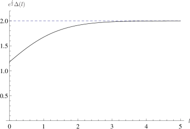
Figure 11: The function $\Delta(l)\,e^{\frac{l}{2}}$ is depicted. It increases monotonically as a function of $l$ from $\frac{3\pi}{8}$ to $2$ for the interval $l\in[0,\infty)$.

For ${\cal I}(x,-\cosh l)$, let us restrict the argument in the range $0\leq x<e^{-l}$. One then get

$${\cal I}(x,-\cosh l)=\frac{1}{\sinh^{2}l}\left(e^{l\over 2}(\sinh l\ F(\sin^{-1}\sqrt{xe^{l}},e^{-2l})-\cosh l\ E(\sin^{-1}\sqrt{xe^{l}},e^{-2l}))\right.$$

$$\quad\quad\quad\quad\quad\quad\left.+\frac{\sqrt{x}(1-x\cosh l)}{\sqrt{1+x^{2}-2x\cosh l}}\right).$$ (A.5)

Appendix B Relation between $a^{c}_{h}(x,y)$ and $b^{c}_{h}(x,y)$

In this appendix, we show the relation

$$a^{c}_{h}=b^{c}_{h}\sin^{2}y-\sin y\cos y\,\partial_{x}b^{c}_{h}$$ (B.1)

for the homogeneous part of the cross-term solution

$$a_{h}^{c}(x,y)=-\frac{(m-m^{-1})\,\sqrt{{R}(m)}}{\sqrt{1+X^{2}}\sqrt{1+Y^{2}}},$$ (B.2)

$$b_{h}^{c}(x,y)=-\frac{4(m-m^{-1})}{\sqrt{R(m)}}$$ (B.3)

with

$$R(m)\equiv m+m^{-1}+2\cosh l.$$ (B.4)

Let us note first

$$\partial_{x}\ln m=-\frac{\cot y}{2}\frac{m-m^{-1}}{\sqrt{1+X^{2}}\sqrt{1+Y^{2}}}.$$ (B.5)

Then

$$\sqrt{1+X^{2}}\sqrt{1+Y^{2}}\,\partial_{x}b^{c}_{h}=\frac{m-m^{-1}}{R^{\frac{3}{2}}(m)}\left[2\big{(}m+m^{-1}\big{)}R(m)-\big{(}m-m^{-1}\big{)}^{2}\right]\cot y.$$ (B.6)

Inserting this into (B.1) with (B.3), one gets

$$\sqrt{1+X^{2}}\sqrt{1+Y^{2}}\,a^{c}_{h} = -\frac{m-m^{-1}}{R^{\frac{3}{2}}(m)}\left[\ 4\sin^{2}y\sqrt{1+X^{2}}\sqrt{1+Y^{2}}\,R(m)\right.$$ (B.7)

$$\left.+\cos^{2}y\Big{(}2(m+m^{-1})R(m)-(m-m^{-1})^{2}\Big{)}\right].$$

Now using the following identity,

$$X^{2}+Y^{2}=2XY\cosh l+\frac{\sinh^{2}l}{\sin^{2}y}$$ (B.8)

one can show

$$4XY\,R(m)=(m-m^{-1})^{2}-4\frac{\sinh^{2}l}{\sin^{2}y},$$ (B.9)

$$4\sqrt{1+X^{2}}\sqrt{1+Y^{2}}\,R(m)=2R(m)(m+m^{-1})-(m-m^{-1})^{2}+4\frac{\sinh^{2}l}{\sin^{2}y}.$$ (B.10)

Inserting (B.10) into (B.7), one recovers the expression for $a^{c}_{h}$ in (B.2).

Appendix C Evaluation of the integral for $\delta x_{B}$

In this appendix, we shall evaluate the integral

$$U(l)\equiv\int^{l}_{\frac{l}{2}}dx\,b^{c}_{0}(x)$$ (C.1)

where

$$b_{0}^{c}(x)=\frac{4}{R(m_{0})}\left[2m_{0}-G_{h}(m_{0})\Big{(}{\cal I}(m_{0})-\frac{\Delta(l)}{2}\Big{)}\right]$$ (C.2)

with $m_{0}$ given in (6.54). First note that

$$m^{\prime}_{0}(x)=-\frac{\sinh l}{\sinh^{2}x}=-\frac{m_{0}R(m_{0})}{\sinh l}.$$ (C.3)

Using the change of variable, the integral is rearranged as

$$U(l)=4\sinh l\int_{0}^{1}\frac{dm_{0}}{R^{2}(m_{0})}\left(2+(1-m^{-2}_{0})R^{\frac{1}{2}}(m_{0})\Big{(}{\cal I}(m_{0})-\frac{\Delta(l)}{2}\Big{)}\right).$$ (C.4)

We use the mathematical identity

$$\frac{1-m^{-2}_{0}}{R^{\frac{3}{2}}(m_{0})}\Big{(}{\cal I}(m_{0})-\frac{\Delta(l)}{2}\Big{)}=-\frac{2}{R^{2}(m_{0})}-\frac{d}{dm_{0}}\frac{1}{R^{\frac{1}{2}}(m_{0})}\Big{(}{\cal I}(m_{0})-\frac{\Delta(l)}{2}\Big{)}.$$ (C.5)

The integral becomes

$$U(l)=4\sinh l\left[4\int^{1}_{0}\frac{dm_{0}}{R^{2}(m_{0})}-\frac{\Big{(}{\cal I}(1)-\frac{\Delta(l)}{2}\Big{)}}{\cosh\frac{l}{2}}\right].$$ (C.6)

We note that

$${\cal I}(1)-\frac{\Delta(l)}{2}=-\frac{1}{2\cosh\frac{l}{2}}$$ (C.7)

and

$$4\int^{1}_{0}\frac{dm_{0}}{R^{2}(m_{0})}=\frac{\sinh l-l}{\sinh^{3}l}.$$ (C.8)

Therefore, one is led to

$$U(l)=4\left(\coth l-\frac{l}{\sinh^{2}l}\right).$$ (C.9)

References

- [1] D. Bak, M. Gutperle and S. Hirano, “A Dilatonic deformation of AdS(5) and its field theory dual,” JHEP 0305, 072 (2003) [hep-th/0304129].
- [2] J. M. Maldacena, “The Large N limit of superconformal field theories and supergravity,” Adv. Theor. Math. Phys. 2, 231 (1998) [hep-th/9711200].
- [3] S. S. Gubser, I. R. Klebanov and A. M. Polyakov, “Gauge theory correlators from non-critical string theory,” Phys. Lett. B 428 (1998) 105 [arXiv:hep-th/9802109].
- [4] E. Witten, “Anti-de Sitter space and holography,” Adv. Theor. Math. Phys. 2 (1998) 253 [arXiv:hep-th/9802150].
- [5] E. D’Hoker, J. Estes and M. Gutperle, “Exact half-BPS Type IIB interface solutions. I. Local solution and supersymmetric Janus,” JHEP 0706 (2007) 021 [arXiv:0705.0022 [hep-th]].
- [6] E. D’Hoker, J. Estes, M. Gutperle and D. Krym, “Exact Half-BPS Flux Solutions in M-theory. I: Local Solutions,” JHEP 0808 (2008) 028 [arXiv:0806.0605 [hep-th]].
- [7] M. Chiodaroli, M. Gutperle and D. Krym, “Half-BPS Solutions locally asymptotic to AdS(3) x S**3 and interface conformal field theories,” JHEP 1002 (2010) 066 [arXiv:0910.0466 [hep-th]].
- [8] E. D’Hoker, J. Estes and M. Gutperle, “Gravity duals of half-BPS Wilson loops,” JHEP 0706 (2007) 063 [arXiv:0705.1004 [hep-th]].
- [9] A. Clark and A. Karch, “Super Janus,” JHEP 0510, 094 (2005) [arXiv:hep-th/0506265].
- [10] O. Lunin, “1/2-BPS states in M theory and defects in the dual CFTs,” JHEP 0710, 014 (2007) [arXiv:0704.3442 [hep-th]].
- [11] J. Kumar and A. Rajaraman, “Supergravity solutions for branes,” Phys. Rev. D 69 (2004) 105023 [arXiv:hep-th/0310056].
- [12] M. Chiodaroli, E. D’Hoker, Y. Guo and M. Gutperle, “Exact half-BPS string-junction solutions in six-dimensional supergravity,” arXiv:1107.1722 [hep-th].
- [13] D. Bak, M. Gutperle and S. Hirano, “Three dimensional Janus and time-dependent black holes,” JHEP 0702 (2007) 068 [arXiv:hep-th/0701108].
- [14] D. Bak, M. Gutperle and A. Karch, “Time dependent black holes and thermal equilibration,” JHEP 0712, 034 (2007) [arXiv:0708.3691 [hep-th]].
- [15] D. Bak, M. Gutperle and R. A. Janik, “Janus Black Holes,” JHEP 1110, 056 (2011) [arXiv:1109.2736 [hep-th]].
- [16] D. Bak, “Dual of big-bang and big-crunch,” Phys. Rev. D 75, 026003 (2007) [arXiv:hep-th/0603080].
- [17] T. Takayanagi, “Holographic Dual of BCFT,” Phys. Rev. Lett. 107, 101602 (2011) [arXiv:1105.5165 [hep-th]].
- [18] M. Fujita, T. Takayanagi and E. Tonni, “Aspects of AdS/BCFT,” JHEP 1111, 043 (2011) [arXiv:1108.5152 [hep-th]].
- [19] A. B. Clark, N. Crossette, G. M. Newman and A. Rommal, “AdS-Sliced Flavor Branes and Adding Flavor to the Janus Solution,” arXiv:1309.7872 [hep-th].
- [20] M. Banados, C. Teitelboim and J. Zanelli, “The Black hole in three-dimensional space-time,” Phys. Rev. Lett. 69, 1849 (1992) [arXiv:hep-th/9204099].
- [21] S. de Haro, S. N. Solodukhin and K. Skenderis, “Holographic reconstruction of space-time and renormalization in the AdS / CFT correspondence,” Commun. Math. Phys. 217, 595 (2001) [arXiv:hep-th/0002230].
- [22] S. Bhattacharyya, V. E. Hubeny, R. Loganayagam, G. Mandal, S. Minwalla, T. Morita, M. Rangamani, H. S. Reall, “Local Fluid Dynamical Entropy from Gravity,” JHEP 0806 (2008) 055. [arXiv:0803.2526 [hep-th]].
- [23] I. Affleck and A. W. W. Ludwig, “Exact critical theory of the two impurity Kondo model,” Phys. Rev. Lett. 68, 1046 (1992).
- [24] I. Affleck, “Conformal field theory approach to the Kondo effect,” Acta Phys. Polon. B 26, 1869 (1995) [cond-mat/9512099].
- [25] J. Malecki, E. Sela and I. Affleck, “Crossover in the two-impurity Kondo model induced by direct charge tunneling,” Phys. Rev. B 82, 205327 (2010) [arXiv:1009.0860 [cond-mat.mes-hall]].
- [26] S. Kachru, A. Karch and S. Yaida, “Holographic Lattices, Dimers, and Glasses,” Phys. Rev. D 81, 026007 (2010) [arXiv:0909.2639 [hep-th]].
- [27] G. T. Horowitz, J. E. Santos and D. Tong, “Optical Conductivity with Holographic Lattices,” JHEP 1207, 168 (2012) [arXiv:1204.0519 [hep-th]].
- [28] N. Iizuka and K. Maeda, “Towards the Lattice Effects on the Holographic Superconductor,” JHEP 1211, 117 (2012) [arXiv:1207.2943 [hep-th]].
- [29] G. T. Horowitz, J. E. Santos and D. Tong, “Further Evidence for Lattice-Induced Scaling,” JHEP 1211, 102 (2012) [arXiv:1209.1098 [hep-th]].
- [30] J. de Boer, “Six-dimensional supergravity on S**3 x AdS(3) and 2-D conformal field theory,” Nucl. Phys. B 548, 139 (1999) [hep-th/9806104].
- [31] S. Ryu and T. Takayanagi, “Holographic derivation of entanglement entropy from AdS/CFT,” Phys. Rev. Lett. 96 (2006) 181602 [arXiv:hep-th/0603001].
- [32] S. Ryu and T. Takayanagi, “Aspects of holographic entanglement entropy,” JHEP 0608 (2006) 045 [arXiv:hep-th/0605073].
- [33] T. Azeyanagi, A. Karch, T. Takayanagi and E. G. Thompson, “Holographic Calculation of Boundary Entropy,” JHEP 0803 (2008) 054 [arXiv:0712.1850 [hep-th]].
- [34] P. Calabrese and J. L. Cardy, “Entanglement entropy and quantum field theory,” J. Stat. Mech. 0406 (2004) P002 [arXiv:hep-th/0405152].
- [35] I. Affleck and A. W. W. Ludwig, “Universal noninteger ’ground state degeneracy’ in critical quantum systems,” Phys. Rev. Lett. 67 (1991) 161.
- [36] M. Chiodaroli, M. Gutperle and L. Y. Hung, “Boundary entropy of supersymmetric Janus solutions,” JHEP 1009, 082 (2010) [arXiv:1005.4433 [hep-th]].
- [37] M. Chiodaroli, M. Gutperle, L. -Y. Hung, D. Krym, “String Junctions and Holographic Interfaces,” Phys. Rev. D83, 026003 (2011). [arXiv:1010.2758 [hep-th]].