NuSTAR Observations of GRB $130427$A establish a single component synchrotron afterglow origin for the late optical to multi-GeV emission

Abstract

GRB 130427A occurred in a relatively nearby galaxy; its prompt emission had the largest GRB fluence ever recorded. The afterglow of GRB 130427A was bright enough for the Nuclear Spectroscopic Telescope ARray (NuSTAR) to observe it in the 3 –$\,79\;$keV energy range long after its prompt emission ($\sim$1.5 and 5 days). This range, where afterglow observations were previously not possible, bridges an important spectral gap. Combined with Swift, Fermi and ground-based optical data, NuSTAR observations unambiguously establish a single afterglow spectral component from optical to multi-GeV energies a day after the event, which is almost certainly synchrotron radiation. Such an origin of the late-time Fermi/LAT $>$10 GeV photons requires revisions in our understanding of collisionless relativistic shock physics.

NuSTAR observations of GRB 1304127A establish

1. Introduction

Gamma-Ray Bursts (GRBs) release within seconds to minutes more high-energy photons than any other transient phenomenon (Kouveliotou et al., 2012). Their prompt gamma-ray emission is followed by a long-lived (typically weeks to months) afterglow, visible from radio to X-rays. The afterglow emission is attributed to synchrotron radiation from relativistic electrons accelerated in the shock produced as the explosion plows into the circumstellar medium. The afterglow synchrotron origin is supported by their broadband spectra (Granot & Sari, 2002; Galama et al., 1998) and polarization measurements (Covino et al., 2004).

GRB 130427A triggered the Fermi/Gamma-ray Burst Monitor (GBM) at 07:47:06.42 UT on 2013 April 27 (von Kienlin, 2013). The intensity and hardness of the event fulfilled the criteria for an autonomous slew maneuver to place the burst within the Fermi/Large Area Telescope (LAT) field-of-view. Its exceedingly bright prompt emission was also detected by other satellites (AGILE: Verrecchia et al. 2013, Konus-Wind: Golenetskii et al. 2013, RHESSI: Smith et al. 2013, Swift: Maselli et al. 2013) and enabled multiple ground- and space-based follow-up observations, allowing for rapid accurate determination of the event location and distance at redshift $z=0.340$ (Levan et al., 2013), as well as extensive broad band afterglow monitoring from radio to $\gamma$-rays. The extreme X-ray and $\gamma$-ray energetics of the burst are described in detail in Preece et al. (2013); Ackermann et al. (2013); Maselli et al. (2013). The record-breaking duration of the LAT afterglow ($\sim$0.1–100 GeV), which lasted almost a day after the GBM trigger, placed GRB 130427A at the top of the LAT GRBs in fluence (Ackermann et al., 2013).

The extreme intensity, accurate distance measurement and relative closeness of GRB 130427A, made it an ideal candidate for follow-up observations with NuSTAR (Harrison et al., 2013). Here we describe our NuSTAR afterglow observations taken during two epochs (§ 2), combined with data from Fermi/LAT, Swift, and optical observatories. We describe in § 3 the derivation of the Fermi/LAT extrapolation and upper limits during the NuSTAR epochs. In § 4 we present afterglow multi-wavelength fits, and discuss our results in § 5.

2. NuSTAR Observations

NuSTAR was launched on 2012 June 13; the instrument’s two telescopes utilize a new generation of hard X-ray optics and detectors to focus X-rays in the range 3 – 79 keV. We observed GRB 130427A at three epochs, starting approximately 1.2, 4.8 and 5.4 days after the GBM trigger, for 30.5, 21.2, and 12.3 ks (live times). We detected the source in all epochs, obtaining for the first time X-ray observations of a GRB afterglow above 10 keV. The NuSTAR data thus provide an important missing spectral link between the Swift/X-Ray Telescope (XRT) observations (0.3 – 10 keV) (Maselli et al., 2013) and the Fermi/LAT observations ($>100\;$MeV) (Ackermann et al., 2013).

We processed the data with HEASOFT 6.13 and the NuSTAR Data Analysis Software (NuSTARDAS) v. 1.1.1 using CALDB version 20130509. We extracted source lightcurves and spectra from circular regions with 75^′′ radius from both NuSTAR modules for the first epoch and 50^′′ radius for the second and third epochs. We used circular background regions (of 150^′′, 100^′′, and 100^′′ radius for each epoch, respectively) located on the same NuSTAR detector as the GRB. Hereafter, we combine the second and third NuSTAR epochs, which were very close in time, to increase the signal-to-noise ratio, and refer to it as the second epoch.

Fig. 1 demonstrates the temporal behavior of the multi-wavelength afterglow flux of GRB 130427A. Here we have included data from Swift/XRT, Swift/UVOT, and Fermi/LAT. We also include the extrapolated Fermi/LAT lightcurve derived as described in § 3. The weighted average of the decay rates during the two NuSTAR epochs (single power-law fits) is $\alpha=1.3$ from optical to GeV (see also the figure inset, and the indices next to each instrument in Fig. 1). We discuss the implications of the temporal results in § 5.

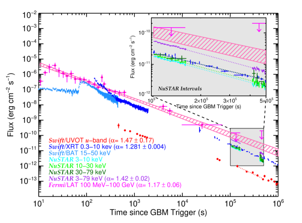
Figure 1.— Lightcurves of GRB 130427A. (Maselli et al., 2013; Ackermann et al., 2013). All errors are 1$\sigma$. The inset zooms in on the NuSTAR epochs. The LAT ULs are shown as arrows and the LAT extrapolated region as a shaded rectangle (1$\sigma$). Numbers in parentheses are indices of power-law fits during the NuSTAR epochs.

3. Fermi Observations

The Fermi/LAT detected GRB 130427A up to almost a day after the trigger time (Fig. 1; Ackermann et al. 2013). Fermi/LAT was also observing during both NuSTAR epochs but did not detect the source. We analyzed the “Pass 7” data with the Fermi Science Tools v9r31p1 and the P7SOURCE_V6 version of the instrument response functions, and using the public Galactic diffuse model and the isotropic spectral template available at http://fermi.gsfc.nasa.gov/ssc/. For each epoch, we selected all the events within a Region Of Interest (ROI) with a radius of 10^∘ around the position of the GRB, excluding times when any part of the ROI was at a zenith angle $>100{{}^{\circ}}$. The latter requirement greatly reduces contamination from the diffuse gamma-ray emission originating from the Earth’s upper atmosphere, peaking at a zenith angle of $\sim$110^∘.

3.1. Fermi/LAT spectra and upper limits

For each epoch we performed an unbinned likelihood analysis over the whole energy range (0.1 – 100 GeV), using a model composed of the two background components (Galactic and isotropic) and a point source with a power-law (PL) spectrum (the GRB), plus the contribution from all the known gamma-ray point sources in the ROI (Nolan et al., 2012). We did not obtain a detection in either epoch, and so we computed upper limits (ULs). We froze the normalization of the background components, and fixed the photon index of the GRB model to $2.17$, which is the best fit value from the smoothly-broken power-law (SBPL) fit during the first NuSTAR epoch as reported in § 4 (the ULs change by less than 10% for any choice of the photon index between $2$ and $2.5$). We then independently fit the GRB model in 3 energy bands ($0.1-1$, $1-10$ and $10-100\;$GeV), using an unbinned profile likelihood method to derive the corresponding 95% LAT ULs (Ackermann et al., 2012). The information contained in such ULs is important to constrain the spectrum, but cannot be handled by a standard fitting procedure. We, therefore, turn to an alternative (but equivalent) method to include the LAT observations in a broadband spectral fit. We obtained the count spectrum of the observed LAT signal (source+background) using gtbin, and the background spectrum using gtbkg, which computes the predicted counts from all the components of the best fit likelihood model except the GRB. Since there is no significant excess above the background, the two spectra are compatible within the errors, although they are not identical. We also ran gtrspgen to compute the response of the instrument in the interval of interest, and loaded these files in XSPEC v.12.7. This software compares the observed net counts to the number of counts predicted by the model folded with the response of the instrument. By minimizing a statistic based on the Poisson probability we can treat equivalently a spectrum containing a significant signal, and a spectrum which is compatible with being just background. While the former will constrain the model to pass through the data points, the latter will constrain it to predict a number of counts above background compatible with zero. The best-fit model obtained using the LAT spectra computed in this way is, as expected, below the ULs computed with the profile likelihood method.

3.2. Extrapolation of the Fermi/LAT lightcurve

The high-energy ($>100\;$MeV) photon and energy flux lightcurves are well described by a broken power law (BPL) and PL, respectively, as reported in Ackermann et al. (2013). To extrapolate such lightcurves to the NuSTAR epochs we adopted a general approach, based on the well-known Markov Chain Monte Carlo technique, which takes into account the uncertainties on the best fit parameters along with all their correlations, as follows.

Each data point in Fig. 2 represents a photon flux derived from a likelihood fit with 1$\sigma$ confidence intervals (Ackermann et al., 2013). Hence, we can assume a Gaussian joint likelihood $L$ and minimize the corresponding $-\log(L)$ to find the best-fit parameters, which is equivalent to a standard least-squares fit (or to minimize $\chi^{2}$). We can then apply the Bayes rule that the posterior distribution for the parameters is directly proportional to the prior distribution multiplied by the likelihood. If we take an uninformative prior, then the posterior distribution is directly proportional to the likelihood itself. Therefore, sampling the likelihood function with a Markov Chain Monte Carlo technique is equivalent to sampling the posterior distribution. By using e.g., the Goodman & Weare (2010) algorithm, we can then obtain many sets of parameters distributed as in the posterior distribution, with all the relations between them taken into account. Using these sets of parameters, $p_{\rm i}$, we can build a distribution of a certain quantity of interest $f(p_{\rm i})$. Taking the median and the relevant percentiles of the distribution we can then extract a measure of $f$ and its 1$\sigma$ confidence interval. In this way, we computed the shaded region in Fig. 2 and the expected flux only in the first NuSTAR epoch, which starts shortly after the last detection from Fermi/LAT. The second NuSTAR epoch started too late for any extrapolation to be meaningful.

Fig. 2 exhibits the Fermi/LAT photon flux lightcurve with 1$\sigma$ confidence intervals derived with such method. We used the same method to compute the flux extrapolation for the first NuSTAR epoch (the magenta dashed cross in Fig. 3).

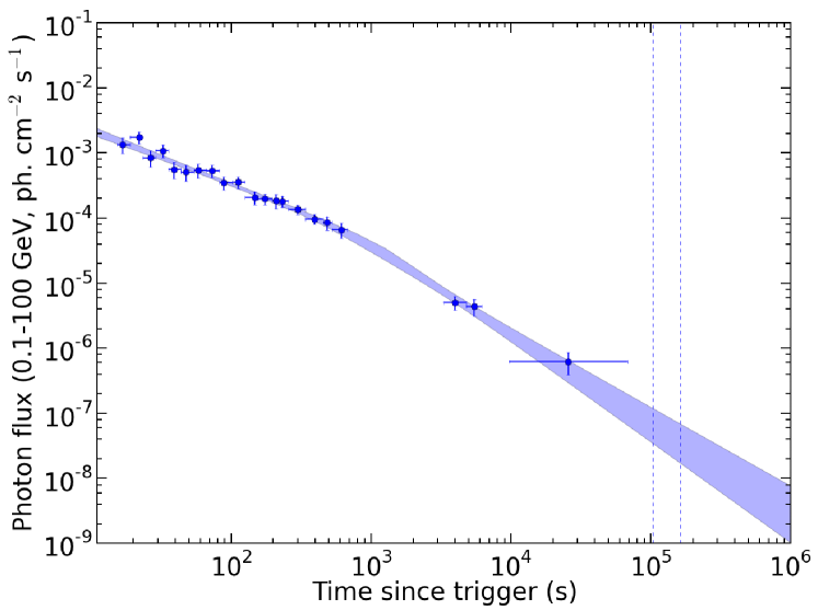
Figure 2.— The decaying part of the Fermi/LAT photon flux lightcurve of the afterglow of GRB 130427A (100 MeV – 100 GeV; Ackermann et al. 2013). The shaded blue region marks the 1$\sigma$ contour for the best-fit BPL model, while the dashed lines indicate the start and stop time for the first NuSTAR epoch. Only data points used for the BPL fit (i.e., after $T_{0}+16\;$s) are included.

4. Broadband Afterglow

We extracted lightcurves and spectra during the NuSTAR epochs from Swift/Ultra-Violet/Optical Telescope (UVOT), and Swift/XRT using the standard HEASOFT reduction pipelines and the Swift/XRT team repository (Evans et al., 2009), as well as Liverpool Telescope data using in-house software (Maselli et al., 2013). For the first epoch, we compare the extrapolation of the LAT temporal and spectral behavior (Ackermann et al., 2013) to our multi-wavelength lightcurves and spectra.

Fig. 3 shows two Spectral Energy Distributions (SEDs) spanning from optical (i’ band) to $\gamma$-rays ($\sim$GeV). We first fit both epochs independently (excluding Fermi/LAT data) with two functional forms (Table 1) – single PL and BPL – each multiplied by models for both fixed Galactic and free intrinsic (host) extinction (zdust) and absorption (phabs), respectively, and a free cross-calibration constant. We find that both epochs can be fit with a PL; however, the second epoch fit is better ($\chi^{2}=1.01$ versus 1.08 for the first epoch). For the first epoch a BPL is significantly better, with an F-test-value of 19.1 (chance probability $P=1.6\times 10^{-8}$, see also Table 1).

We then fit the first epoch only with a physically motivated SBPL spectrum described in Granot & Sari (2002), with a fixed sharpness of the break, $s=0.85$, and including the broadband LAT UL. We performed two fits: (i) keeping the two power-law indices free, and (ii) requiring them to differ by $\Delta\Gamma=0.5$ according to the synchrotron radiation theoretical expectation (Granot & Sari, 2002). The SBPL fit was better (Table 1) and is shown at the top panel of Fig. 3, together with the LAT ULs, as well as the extrapolation of the LAT lightcurve to this epoch; the extrapolation was not used in the fit but plotted for comparison with the model. Both are consistent with the SBPL fit – the curvature in the NuSTAR data is also clearly exhibited in the inset in the top panel. The lower panel shows the SED with the second NuSTAR epoch fit with a PL and with the first epoch fit shifted and superposed on the plot; although the data do not constrain such a fit, they are consistent with it. Finally, we performed broadband fits removing the NuSTAR data (including only optical, Swift/XRT, Swift/UVOT data, and Fermi/LAT ULs) and found that the break energies could not be constrained. Therefore, the NuSTAR data are essential in constraining the shape of the broadband spectra.

Our results are broadly consistent with those of Perley et al. (2013) who derived radio to GeV afterglow spectra of GRB 130427A covering $0.007-60\;$days after trigger. Their results also suggest that the forward shock emission indeed dominates at or above the optical during our NuSTAR epochs.

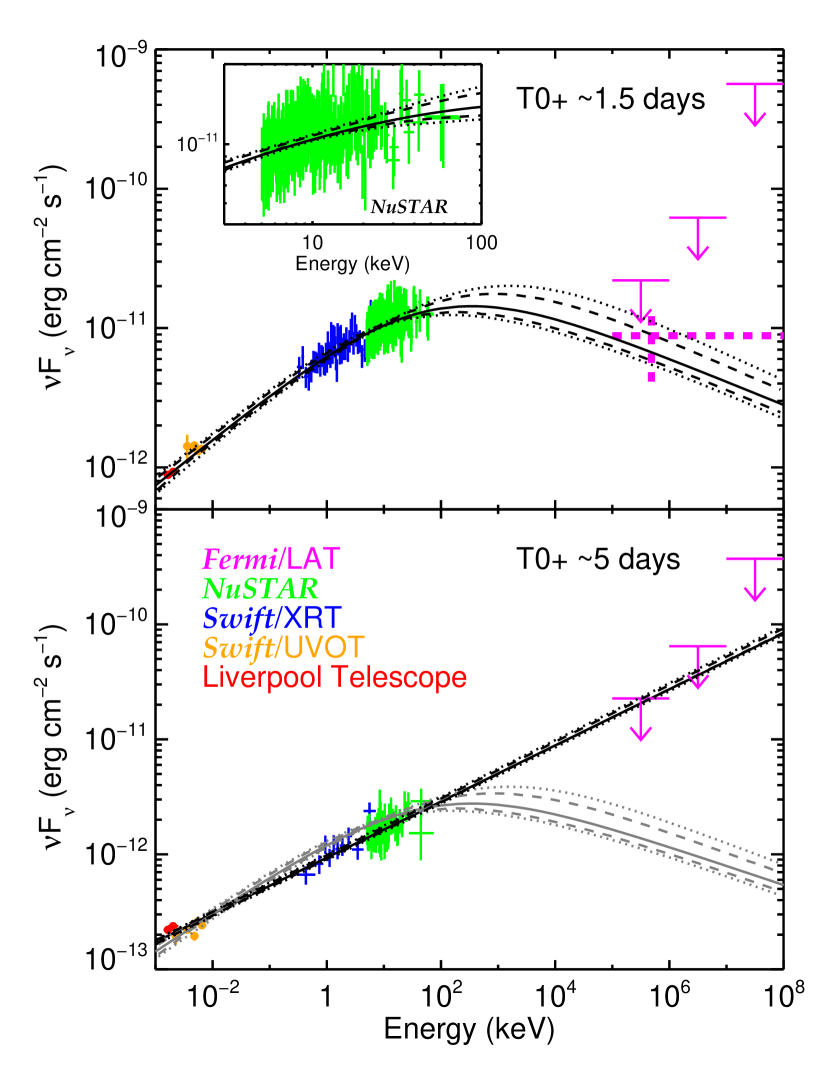
Figure 3.— The optical to GeV spectrum of GRB 130427A fit with a SBPL synchrotron model (Granot & Sari, 2002). Broad-band SEDs are shown during the first (top-panel) and the second (bottom-panel) NuSTAR epochs. The Fermi/LAT ULs are shown as arrows and the extrapolation of the LAT flux light curve is shown as a dashed magenta cross (only during the first epoch). The second epoch (bottom-panel) is fit with a PL (black lines); the fit to the first epoch is scaled down and superposed on the second epoch data for comparison (in gray).The optical/UV/XRT data are corrected for absorption and Galactic extinction. All data point errors are 1$\sigma$; the LAT ULs are 2$\sigma$; the error contours are 2$\sigma$ (dashed lines) and 3$\sigma$ (dotted lines).

Table 1Broadband Spectral Fits during the NuSTAR Epochs

Model	Epoch	O+X	N	L	$\Delta\Gamma$	$\Gamma_{1}$	$\Gamma_{2}$	$E_{c}$	$\chi^{2}/$d.o.f.
PL	1	yes	yes	-	-	$1.72\pm 0.02$	-	-	457.6/422
PL	2	yes	yes	-	-	$1.77\pm 0.02$	-	-	105.1/104
BPL	1	yes	yes	-	free	$1.70\pm 0.01$	$1.89^{+0.08}_{-0.04}$	$9.3^{+2.3}_{-1.4}$	419.3/420
BPL	2	yes	yes	-	free	$1.77$	-	-	-
BPL	1	yes	yes	-	0.5	$1.71\pm 0.01$	2.21	$17\pm 1$	428.5/421
BPL	2	yes	yes	-	0.5	$1.77\pm 0.01$	2.27	$32^{+14}_{-8}$	103.7/103
Fits to Optical+X-ray+NuSTAR +LAT confirm presence of break and demonstrate best fit physical model
PL	1	yes	yes	UL	-	$1.72\pm 0.01$	-	-	489.1/434
PL	2	yes	yes	UL	-	$\bf 1.76\pm 0.01$	-	-	130.6/116
BPL	1	yes	yes	UL	free	$1.70\pm 0.01$	$1.91\pm 0.03$	$9.4^{+1.4}_{-0.9}$	428.5/432
SBPL	1	yes	yes	UL	free	$1.69\pm 0.01$	$2.91^{+0.53}_{-0.49}$	$96^{+51}_{-25}$	422.7/430
SBPL	1	yes	yes	UL	0.5	$\bf 1.67\pm 0.01$	2.17	$70^{+59}_{-31}$	427.7/429

5. Discussion

We have shown above that the NuSTAR data are consistent with a power law in time and frequency below the cooling-break photon energy $E_{c}$, $F_{\nu}\propto t^{-\alpha}\nu^{-\beta}$ with $\alpha=1.30\pm 0.05$ and $\beta\equiv\Gamma_{1}-1=0.69\pm 0.01$ (see Table 1). For the likely power-law segment (G from Granot & Sari 2002) of the synchrotron spectrum this implies a power-law index of the external medium density, $\rho_{\rm ext}\propto{}R^{-k}$, where $R$ is the distance from the central source, of $k=4/[1+1/(2\alpha-3\beta)]=1.4\pm 0.2$. Correspondingly, the cooling-break energy scales as $E_{c}\propto{}t^{(3k-4)/(8-2k)}=t^{0.05\pm 0.12}$, i.e., it is expected to remain constant (which is consistent with our spectral fits, the difference between the two epochs being less than 2$\sigma$). The value we obtain for $k$ is intermediate between a uniform interstellar medium ($k=0$) and a canonical massive-star wind ($k=2$), possibly indicating that the massive GRB progenitor has produced an eruption (e.g., is opacity driven) prior to its core-collapse, which alters the circumstellar density profile (Fryer at al., 2006). Such an eruption might also account for a variable external density profile, where a transition from a flatter profile to a steeper one might be responsible for the steepening of the optical-to-X-ray lightcurves after several hours (Ackermann et al., 2013; Laskar et al., 2013). The density profile might have been relatively steep ($k\sim 1-2$) during the first few hundred seconds, shortly after the outflow deceleration time, possibly accounting for the early reverse shock emission (Laskar et al., 2013; Perley et al., 2013).

The NuSTAR power-law distributions in time and frequency support an afterglow synchrotron origin (Kumar & Barniol Duran, 2009, 2010; Ghisellini et al., 2010). Synchrotron radiation models predict a maximum synchrotron photon energy, $E_{\rm{}syn,max}$, derived by equating the electron acceleration and synchrotron radiative cooling timescales, assuming a single acceleration and emission region (Guilbert et al., 1983; de Jager et al., 1996; Kirk & Reville, 2010; Piran & Nakar, 2010). In the context of late-time Fermi/LAT high-energy photons, this was first briefly mentioned as a problem for a synchrotron origin for GRB 090902B (Abdo et al., 2009), and later discussed more generally and in depth by Piran & Nakar (2010). The long-lasting ($\sim$1 day) Fermi/LAT afterglow included a 32 GeV photon after 34 ks, and altogether five $>$30 GeV photons after $>$200 s. All five significantly exceed $E_{\rm{}syn,max}$, by factors of 6–25 for $k=0$, and 9–20 for $k=2$ (using Eq. (4) of Piran & Nakar, 2010). This led to suggestions that the Fermi/LAT high-energy photons were not synchrotron radiation, but instead arose from a distinct high-energy spectral component (Ackermann et al., 2013; Fan et al., 2013).

Such a component may arise for example, from synchrotron self-Compton (Fan et al., 2013). This mechanism was predicted to dominate at high photon energies at late times (Panaitescu & Kumar, 2000; Sari & Esin, 2001), but has rarely been detected in the late X-ray afterglow (Harrison et al., 2001; Yost et al., 2002). Other possible origins of the high-energy emission involve long-lived activity of the central source, producing a late relativistic outflow that provides seed synchrotron photons or relativistic electrons that might scatter either their own synchrotron emission or that of the afterglow shock (Fan & Piran, 2008). In GRB 130427A, however, there are no signs of prolonged central source activity (such as X-ray flares) beyond hundreds of seconds. Another option is a “pair echo” involving TeV photons emitted promptly by the GRB, which pair-produce with photons of the extragalactic background light; for low enough intergalactic magnetic fields the resulting pairs can produce detectable longer-lived GeV emission by up-scattering cosmic microwave background photons (Plaga, 1995; Takahashi et al., 2008). However, in this case the flux decay rate is expected to gradually steepen and the photon index to soften, in contrast with observations. A different possibility is pair cascades, induced by shock-accelerated ultra-high-energy cosmic rays (Dermer & Atoyan, 2006).

For any of these alternative models to work, there needs to be a transition from synchrotron emission (at low photon energies) to the alternative model (at high energies). We expect that if a distinct spectral component dominated the emission at GeV energies, it would naturally show up in a broad-band SED. By combining optical, XRT, NuSTAR and Fermi/LAT UL data, we have shown that the SED at $\sim$1.5 days is perfectly consistent with the theoretically expected SBPL spectral shape from optical to GeV energies, without any unaccounted-for flux, and that the flux at all these energies decays at a similar rate. This strongly suggests a single underlying spectral component over a wide energy range. For low energies, the most viable emission mechanism for such a spectral component is synchrotron radiation, suggesting that the entire SED is produced by synchrotron emission.

Therefore, our results strongly suggest that the late-time Fermi/LAT high-energy photons in GRB 130427A are indeed afterglow synchrotron radiation, and provide the strongest direct observational support to date for such an afterglow synchrotron origin of late-time $>$10 GeV Fermi/LAT photons. As was already pointed out (e.g., Piran & Nakar, 2010), such an origin challenges particle acceleration models in afterglow shocks. In particular, at least one of the assumptions in estimating $E_{\rm syn,max}$ must be incorrect, requiring a modification of our understanding of afterglow shock physics. While many authors were aware of this potential problem, the NuSTAR results make it much harder to circumvent. One possible solution may lie in changing the assumption of a uniform magnetic field into a lower magnetic field acceleration region and a higher magnetic field synchrotron radiation region (Kumar et al., 2012; Lyutikov, 2010). These might arise for diffusive shock acceleration (Fermi Type I) if the tangled shock-amplified magnetic field decays on a short length scale behind the shock front (where most of the high-energy radiation is emitted), while the highest energy electrons are accelerated in the lower magnetic field further downstream (Kumar et al., 2012).

Another possibility is direct linear acceleration in the electric field of magnetic reconnection layers, which have a low magnetic field (Uzdensky et al., 2011; Cerutti et al., 2012, 2013). This would require, however, a significant fraction of the total energy in the flow to reside in magnetic fields of alternating sign. This is not expected in GRB afterglows, but it could occur in the magnetic-reconnection induced decay of the tangled shock-amplified field mentioned above, which initially reaches near-equipartition values just behind the shock. While the exact solution is still unclear, our results provide an important challenge for our understanding of particle acceleration and magnetic field amplification in relativistic shocks.

References

- Abdo et al. (2009) Abdo, A. A., et al. 2009, ApJ, 706, L138
- Ackermann et al. (2012) Ackermann, M., et al. 2012, ApJ, 754, 121
- Ackermann et al. (2013) Ackermann, M., et al. 2013, Science, in press (doi:10.1126/science.1242353)
- Cerutti et al. (2012) Cerutti, B., Uzdensky, D., & Begelman, M. C. 2012, ApJ, 746, 148
- Cerutti et al. (2013) Cerutti, B., Werner, G. R., Uzdensky, D. A., & Begelman, M. C. 2013, ApJ, 770, 147
- Covino et al. (2004) Covino, S., Ghisellini, G., Lazzati, D., & Malesani, D. 2004, ASP Conf. Ser., 312, 169
- Dermer & Atoyan (2006) Dermer, C., & Atoyan, A. 2006, New Journal of Physics, 8, 122
- Evans et al. (2009) Evans, P. A., et al. 2009, MNRAS, 397, 1177
- Fan et al. (2013) Fan, Y.-Z., et al. 2013, ApJ, 776, 95
- Fan & Piran (2008) Fan, Y.-Z., & Piran, T. 2008, Front. Phys. Ch., 3, 306
- Fryer at al. (2006) Fryer, C. L., Rockefeller, G., & Young, P. A. 2006, ApJ, 647, 1269
- Galama et al. (1998) Galama, T. J., et al. 1998, ApJ, 500, L97
- Ghisellini et al. (2010) Ghisellini, G., Ghirlanda, G., Nava, L., & Celotti, A. 2010, MNRAS, 403, 926
- Golenetskii et al. (2013) Golenetskii, S., et al. 2013, GCN Circ. 14487
- Goodman & Weare (2010) Goodman, J., & Weare, J. 2010, Communications in Applied Mathematics and Computational Science, 5.1, 65
- Granot & Sari (2002) Granot, J., & Sari, R. 2002, ApJ, 568, 820
- Guilbert et al. (1983) Guilbert, P. W., Fabian, A. C., & Rees, M. J. 1983, MNRAS, 205, 593
- Harrison et al. (2001) Harrison, F. A., et al. 2001, ApJ, 559, 123
- Harrison et al. (2013) Harrison, F. A., et al. 2013, ApJ, 770, 103
- de Jager et al. (1996) de Jager, O. C., et al. 1996, ApJ, 457, 253
- Kirk & Reville (2010) Kirk, J. G., & Reville, B. 2010, ApJ, 710, L16
- Kouveliotou et al. (2012) Kouveliotou, C., Wijers, R.A.M.J., & Woosley, S.E., 2012, Gamma-Ray Bursts, Cambridge University Press.
- Kumar & Barniol Duran (2009) Kumar, P., & Barniol Duran, R. 2009, MNRAS, 400, L75
- Kumar & Barniol Duran (2010) Kumar, P., & Barniol Duran, R. 2010, MNRAS, 409, 226
- Kumar et al. (2012) Kumar, P., Hernández, R. A., Bosnjak, Z., & Barniol Duran, R. 2012, MNRAS, 427, L40
- Laskar et al. (2013) Laskar, T., et al. 2013, ApJ, 776, 119
- Levan et al. (2013) Levan, A., et al. 2013, GCN Circ. 14455
- Lyutikov (2010) Lyutikov, M. 2010, MNRAS, 405, 1809
- Maselli et al. (2013) Maselli, A., et al. 2013, GCN Circ. 14448
- Maselli et al. (2013) Maselli, A., et al. 2013, Science, in press (doi:10.1126/science.1242279)
- Nolan et al. (2012) Nolan, P. L., et al. 2012, ApJS, 199, 31
- Panaitescu & Kumar (2000) Panaitescu, A., & Kumar, P. 2000, ApJ, 543, 66
- Perley et al. (2013) Perley, D. A., et al. 2013, submitted to ApJ (arXiv:1307.4401)
- Piran & Nakar (2010) Piran, T., & Nakar, E. 2010, ApJ, 718, L63
- Plaga (1995) Plaga, R. 1995, Nature, 374, 430
- Preece et al. (2013) Preece, R., et al. 2013, Science, in press (doi:10.1126/science.1242302)
- Sari & Esin (2001) Sari, R., & Esin, A. A. 2001, ApJ, 548, 787
- Smith et al. (2013) Smith, G. M., Csillaghy, A., Hurley, K., et al. 2013, GCN Circ. 14455
- Takahashi et al. (2008) Takahashi, K., Murase, K., Ichiki, K., Inoue, S., & Nagataki, S. 2008, ApJ, 687, L5
- Uzdensky et al. (2011) Uzdensky, D., Cerutti, B., & Begelman, M. C. 2011, ApJ, 737, L40
- Verrecchia et al. (2013) Verrecchia, F., Pittori, C., Giuliani, A., et al. 2013, GCN Circ. 14455
- von Kienlin (2013) von Kienlin, A. 2013, GCN Circ. 14473
- Yost et al. (2002) Yost, S. A., et al. 2002, ApJ, 577, 155