On the Outer Edges of Protoplanetary Dust Disks

Abstract

The expectation that aerodynamic drag will force the solids in a gas-rich protoplanetary disk to spiral in toward the host star on short timescales is one of the fundamental problems in planet formation theory. The nominal efficiency of this radial drift process is in conflict with observations, suggesting that an empirical calibration of solid transport mechanisms in a disk is highly desirable. However, the fact that both radial drift and grain growth produce a similar particle size segregation in a disk (such that larger particles are preferentially concentrated closer to the star) makes it difficult to disentangle a clear signature of drift alone. We highlight a new approach, by showing that radial drift leaves a distinctive “fingerprint” in the dust surface density profile that is directly accessible to current observational facilities. Using an analytical framework for dust evolution, we demonstrate that the combined effects of drift and (viscous) gas drag naturally produce a sharp outer edge in the dust distribution (or, equivalently, a sharp decrease in the dust-to-gas mass ratio). This edge feature forms during the earliest phase in the evolution of disk solids, before grain growth in the outer disk has made much progress, and is preserved over longer timescales when both growth and transport effects are more substantial. The key features of these analytical models are reproduced in detailed numerical simulations, and are qualitatively consistent with recent millimeter-wave observations that find gas/dust size discrepancies and steep declines in dust continuum emission in the outer regions of protoplanetary disks.

1. Introduction

Much of the current research on circumstellar disks is focused on forging links to planet formation, specifically through difficult observational examinations of the disk material within a few tens of AU from its host star. By comparison, the outer reaches of these disks ($\sim$hundreds of AU) receive little attention, despite being more easily accessible to current telescopes (especially at mm/radio wavelengths). Observations of the material at large disk radii are indirectly quite relevant to the planet formation process: the outer disk contains the majority of the mass reservoir available for making planets, and resolved measurements of its structure can potentially reveal clues to some fundamental disk evolution mechanisms (e.g., Andrews et al. 2009, 2010).

In the context of the outer disk, a size seems like a basic property that can be easily inferred. However, resolved observations indicate that such a measurement is problematic: the apparent size depends on the adopted tracer. Radio interferometer data suggest that line emission from abundant molecules (e.g., CO) appears more spatially extended than continuum radiation from dust. In the initial studies of outer disk structures, this discrepancy was dismissed as an artifact of limited continuum sensitivity (Dutrey et al. 1998; Guilloteau & Dutrey 1998). The emission line tracers of molecular gas are highly optically thick, so even a small amount of gas far from the host star still emits at a detectable level (e.g., Beckwith & Sargent 1993). But, the continuum emission at these wavelengths is optically thin (Beckwith et al. 1990), so the corresponding radiation from dust was much too faint for those early observations. However, that explanation proved fleeting when the observed gas/dust size discrepancy persisted even after the sensitivity improved (Piétu et al. 2005, 2007; Isella et al. 2007). An elegant solution proposed by Hughes et al. (2008) showed that a more appropriate model for the density profile in a viscous disk – with an exponential taper at large radii – reconciles the discrepancy (again through an optical depth/sensitivity effect).

Yet, remarkably, the continued improvement in data quality has revealed that even this solution is insufficient. The line/continuum size discrepancies remain an issue, leading some to speculate that there is an intrinsic, physical difference in the radial distributions of gas and dust such that the dust-to-gas mass ratio decreases with distance from the host star (Panić et al. 2009; Andrews et al. 2012; de Gregorio-Monsalvo et al. 2013; Rosenfeld et al. 2013). Moreover, in the best currently available datasets, the continuum emission is found to exhibit a sharp decrease over a narrow radial range ($\Delta r/r\lesssim 0.1$; Andrews et al. 2012; de Gregorio-Monsalvo et al. 2013). This latter feature is tantalizingly reminiscent of the precipitous drop in the population of large bodies in the classical Kuiper Belt $\gtrsim$50 AU from the Sun (Jewitt et al. 1998; Allen et al. 2001; Trujillo et al. 2001). Taken together, these attempts to measure disk sizes have forced observers to suggest that the radial profile of the dust-to-gas ratio features a steep decrease – an “edge” – in the outer regions of a protoplanetary disk. So far, a physical explanation for this feature is lacking, although it has anecdotally been associated with a profound change in the grain properties.

In this article, we develop theoretical models which suggest that both the gas/dust size discrepancy and the sharp dust edges observed in disks at radii of tens or hundreds of AU are natural, generic consequences of the growth and migration of solids in a viscously evolving gas disk. In Sections 2 and 3, we describe our calculations of this evolution in some relevant analytical limits: an “early” phase where an outer dust edge forms rapidly before substantial particle size evolution, and a “late” phase where particles have already reached a maximum equilibrium size. In Section 4, we verify these findings with more sophisticated numerical simulations that track the complete evolution, without these simplifying assumptions. Finally, in Section 5 we discuss the results and highlight how the analysis of resolved continuum and molecular line observations of disks can help empirically calibrate such particle evolution models in the near future.

2. Early Phase

In this section, we consider the radial migration of dust grains in the outer regions of a protoplanetary disk during an “early” phase, where the evolution of particle sizes has not yet progressed enough to significantly affect their dynamics. For simple assumptions about typical collisions, the growth (or size-doubling) timescale can be expressed as (Kornet et al. 2001; Brauer et al. 2008)

$$\tau_{\mathrm{g}}=\frac{1}{\epsilon\,\Omega_{\mathrm{k}}\,S},$$ (1)

with $\epsilon=\Sigma_{\mathrm{d}}/\Sigma_{\mathrm{g}}$ the dust-to-gas surface density ratio, $\Omega_{\mathrm{k}}$ the Keplerian orbital frequency, and $S$ the sticking efficiency (taken to be unity). In the outer disk and for the grain sizes of interest here, the main source of collision velocities is turbulence (Ormel & Cuzzi 2007, but see Section 5). For typical outer disk parameters, estimates of $\tau_{\mathrm{g}}$ (and the duration of this phase) are roughly 0.1 Myr.

There are two primary radial transport mechanisms for dust embedded in a gas disk: (1) radial drift, caused by an angular momentum exchange between dust particles and the sub-Keplerian orbital motion of the gas; and (2) gas drag, produced by the coupling of dust particles in the gas flows controlled by viscous evolution. The dust velocity imparted by drift is (Nakagawa et al. 1986)

$$u_{\mathrm{rd}}=\frac{1}{\mathrm{St}+\mathrm{St}^{-1}}\,\frac{c_{\mathrm{s}}^{2}}{V_{\mathrm{k}}}\frac{\mathrm{dln}P}{\mathrm{dln}r},$$ (2)

with sound speed $c_{\mathrm{s}}$, Keplerian velocity $V_{\mathrm{k}}$, and gas pressure $P$. And the dust velocity introduced by gas drag is

$$u_{\mathrm{gd}}=\frac{1}{1+\mathrm{St}^{2}}\,u_{\mathrm{g}},$$ (3)

with a gas radial velocity

$$u_{\mathrm{g}}=-\frac{3}{\Sigma_{\mathrm{g}}\,\sqrt{r}}\frac{\partial}{\partial r}\left(\Sigma_{\mathrm{g}}\,\nu\,\sqrt{r}\right),$$ (4)

where we assume

$$\nu=\alpha_{\mathrm{t}}\,\frac{c_{\mathrm{s}}^{2}}{\Omega_{\mathrm{k}}}$$ (5)

as a parametrization of the gas viscosity (Shakura & Sunyaev 1973). In Eq. 2, we introduced the Stokes number $\mathrm{St}$, a dimensionless size that characterizes the coupling strength between the dust and gas. The drag force is always in the Epstein regime for the regions of the disk and the particle sizes of interest here. In that case, the Stokes number at the disk mid-plane can be written as

$$\mathrm{St}\simeq\frac{a\,\rho_{\mathrm{s}}}{\Sigma_{\mathrm{g}}}\,\frac{\pi}{2},$$ (6)

where $a$ is the grain radius and $\rho_{\mathrm{s}}$ the internal density of the grain, assumed here to be 1.6 g cm^-3.

To illustrate the dynamical behavior that these transport mechanisms have on dust particles, we need to first adopt a set of representative parameters that characterize the disk structure. The gas temperatures (i.e., sound speeds) influence the dust velocities, and the gas surface densities affect the dust-gas coupling. Here and throughout this article, we assume that the gas surface density profile can be described by the standard, self-similar solution to the viscous evolution equations presented by Lynden-Bell & Pringle (1974) or Hartmann et al. (1998),

$$\Sigma_{\mathrm{g}}(r)=\Sigma_{0}\left(\frac{r}{r_{\mathrm{c}}}\right)^{-\gamma}\exp\left[\left(-\frac{r}{r_{\mathrm{c}}}\right)^{2-\gamma}\right]$$ (7)

(implying the turbulence parameter $\alpha_{\mathrm{t}}$ is constant), and that the temperature follows a power law,

$$T(r)\propto\left(\frac{r}{r_{\mathrm{c}}}\right)^{-q}.$$ (8)

Throughout this article, we assume $\gamma=1$ and $q=1/2$. Although this is not the most general case, it does significantly simplify the calculations we will perform, and finds some support through the modeling of gas emission lines observed in protoplanetary disks (e.g., Andrews et al. 2012). We adopt a set of fiducial model parameters: a stellar host mass of 0.8 M_⊙, initial disk mass of 0.01 M_⊙, initial radius ($r_{c}$) of 20 AU, $\alpha_{\mathrm{t}}$ = $10^{-3}$, initial dust-to-gas ratio ($\epsilon$) of 0.01 at all $r$, and a (fixed) temperature scaling such that $T(\mathrm{1\,AU})=200$ K. Here and in Section 3 we will keep the gas surface densities fixed for clarity, but we permit $\Sigma_{\mathrm{g}}$ to evolve viscously in Section 4.

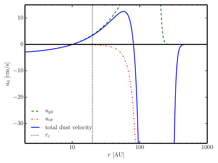
Figure 1.— The early phase radial dust transport velocities for the fiducial model (solid), with the individual contributions from radial drift (dash-dot) and viscous gas drag (dash) shown separately. The initial $r_{\mathrm{c}}$ is marked by a vertical dotted line. Note that inward velocities are negative.

The initial size distribution of the dust incorporated into a disk is thought to resemble the interstellar medium (Mathis et al. 1977, hereafter MRN), perhaps with some growth up to $\mu$m sizes (e.g., Ossenkopf & Henning 1994). A common feature of such size distributions, derived either theoretically (e.g., Tanaka et al. 1996; Birnstiel et al. 2011) or observationally (e.g., MRN), is that most of the mass is contained in the largest grains. Since the transport velocities noted above also increase with grain size, we assume that the effective dust transport velocity is approximately equal to that of the largest grains. Here, we assume an initial size of 1 $\mu$m for the dust particles.

With those assumptions and adopted fiducial parameters, Figure 1 shows the radial velocity distribution of the dust surface density in the early phase, as well as the decomposed contributions from gas drag and radial drift individually, based on Eq. 2 and 3, respectively. In the following sections, we consider in more detail first the effects of drift only (Section 2.1), and then the combined impact of both drift and drag (Section 2.2) on the overall dust dynamics.

2.1. Radial drift only

Youdin & Shu (2002) derived an analytic solution to the advection equation for a case where radial drift is the only transport mechanism, assuming a fixed particle size and a power-law gas surface density profile (of infinite extent). They demonstrated that drift creates an outer boundary in the distribution of mm-sized particles that steepens as it moves in to smaller radii (see also Jacquet et al. 2012). Similarly, Weidenschilling (2003) mentioned the truncation of the dust disk in models which included the growth and radial drift of dust particles.

Here, we extend the work of Youdin & Shu (2002) by recognizing that this mechanism is more general, and applies to much smaller particle sizes if the coupling between the gas and dust is of the right strength. We argue that this is the case in the outer disk, since viscous models have an exponential taper in $\Sigma_{\mathrm{g}}$ rather than a fixed power-law profile that extends indefinitely (see Eq. 7). The corresponding steep decrease in the gas pressure in the outer disk (i.e., the large $\mathrm{d}P/\mathrm{d}r$ in Eq. 2) also enhances the dust/gas coupling (cf., Eq. 6), thereby dramatically boosting the drift velocity of an initial population of small grains.

For small particles with $\mathrm{St}<1$, the drift velocity in Eq. 2 can be approximated as

$$u_{\mathrm{rd}}\simeq-\,\frac{\mathrm{St}_{0}\,c_{\mathrm{c}}^{2}}{V_{\mathrm{c}}}\,\frac{r}{r_{\mathrm{c}}}\left(\frac{r}{r_{\mathrm{c}}}+\frac{11}{4}\right)\,\exp\left(\frac{r}{r_{\mathrm{c}}}\right),$$ (9)

where $\mathrm{St}_{0}$ is the Stokes number for grains of size $a_{0}$ at a surface density $\Sigma_{0}$, and $c_{\mathrm{c}}$ and $V_{\mathrm{c}}$ are the sound speed and Keplerian velocity at $r_{\mathrm{c}}$, respectively. It is immediately clear in Eq. 9 that the inward speed beyond $r_{\mathrm{c}}$ is exponentially rising, becoming much faster than for a power-law $\Sigma_{\mathrm{g}}$ model. This causes even $\mu$m-sized particles to effectively spiral inwards, producing a sharp outer edge in the dust surface density distribution and leaving the very outer disk devoid of dust.

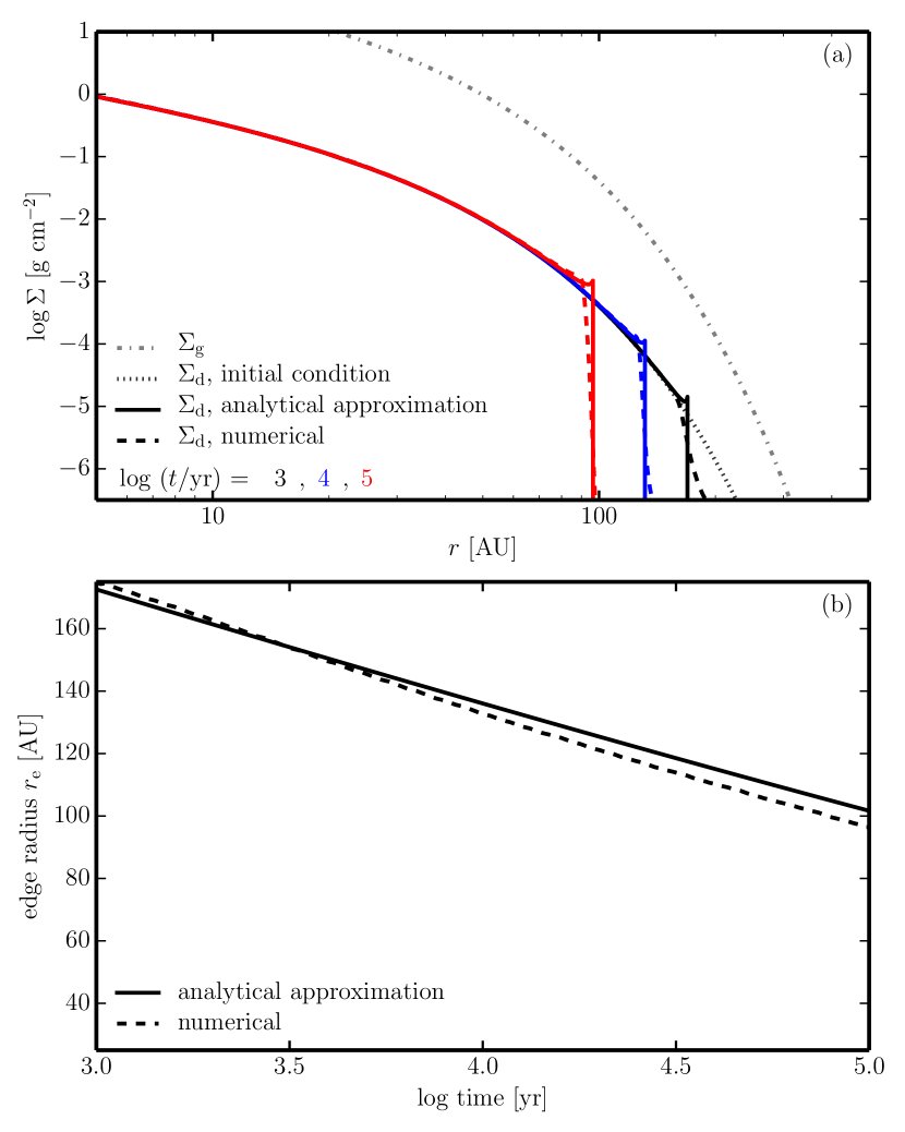
Figure 2.— (a) Analytical (solid) and numerical (dashed) calculations of how radial drift changes the dust surface density profile (cf., Appendix B), leading to the formation of a sharp outer dust edge. The gas surface density profile is shown as a dotted curve. (b) The approximate analytical (solid) and numerical (dashed) evolution of the outer dust edge location, $r_{\mathrm{e}}$ (in units of $r_{\mathrm{c}}$).

After a basic introduction to the relevant dust transport equations (Appendix A), we derive an analytic solution in Appendix B that describes the early evolution of the dust surface densities, $\Sigma_{\mathrm{d}}(r,t)$ (cf., Eq. B7), and the location of this outer dust edge, $r_{\mathrm{e}}(t)$ (cf., Eq. B9). Figure 2 compares these analytic solutions (Eqs. B6, B7, and B9) to a direct, numerical calculation for a single particle size ($a_{0}=1~{}\mu$m). The top panel shows discrete steps in $\Sigma_{\mathrm{d}}(r,t)$, and demonstrates that small dust is quickly removed beyond a sharp outer edge that drifts inward with time. The bottom panel tracks that edge location directly, finding that $r_{\mathrm{e}}(t)$ decreases from $\sim$9 to 5 $r_{\mathrm{c}}$ (in this example, 175 to 100 AU). As a comparison, we evolved the same initial dust distribution for a model with a power-law gas surface density profile, $\Sigma_{\mathrm{g}}=\Sigma_{0}(r/r_{\mathrm{c}})^{-1}$ (not shown in Fig. 2), and confirmed that $\Sigma_{\mathrm{d}}$ does not appreciably change over the $\sim$0.1 Myr timescale on which these calculations are valid. Figure 2 shows slight differences in the edge position between the approximate analytical and numerical solutions: these are entirely due to the approximation used for the dust velocity, which becomes better for smaller $r_{\mathrm{c}}$. Solving Eqns. A6 and A7 using the exact velocity term (as is necessary in the next section) significantly improves their agreement.

It is worth a reminder that these solutions have so far neglected particle size evolution, by assuming a grain size that does not evolve with time. Ultimately, grain growth limits the applicability of our assumptions for this early phase, and effectively bounds the inward motion of the outer dust edge. That limit can be estimated numerically by evaluating Eq. B9 at the growth timescale, $r_{\mathrm{e}}^{\mathrm{min}}\simeq r_{e}(\tau_{\mathrm{g}})$. For our fiducial model, $r_{\mathrm{e}}^{\mathrm{min}}$ is roughly 6 $r_{\mathrm{c}}$, and for reasonable ranges of the key input parameters, we suggest that $r_{\mathrm{e}}^{\mathrm{min}}$ can range between $\sim$3 and 8 $r_{\mathrm{c}}$. At very large distances outside this edge, the gas densities become so low that even small grains have $\mathrm{St}\gg 1$, and therefore the adopted approximations for dust transport in this phase do not apply (at large $\mathrm{St}$, drift velocities are lower than assumed). In our fiducial model, this occurs for $r\gtrsim 14~{}r_{\mathrm{c}}$, although it should be noted that the dust surface densities at such radii are negligibly small. To summarize, the grain growth timescale imposes limits on the applicability of the early phase that can be translated into a specific radial range in the disk; in the case of our fiducial model, that range is $\sim$120–280 AU.

2.2. Radial drift and gas drag

Although we showed in Figure 1 that radial drift dominates the dust motion in the outer disk during the early phase, it is not the only relevant transport mechanism. Dust can also be dragged along with the viscously evolving gas disk. For $\mathrm{St}<1$, this radial motion is approximately equal to Eq. 4. We can get some intuition on how the dust evolves if both radial drift and gas drag are considered together by assuming the same, fixed $\Sigma_{\mathrm{g}}$ as in Eq. 7 and solving for the dust transport equations in Appendix A using the sum of Eq. 2 and Eq. 3 as the effective velocity term. This assumption neglects the effects of evolution in $\Sigma_{\mathrm{g}}$, which would slightly modify the velocity term, but since significant surface density changes occur over the relatively long viscous timescale in the outer disk, these modifications have only a minor effect on the results during the early phase.

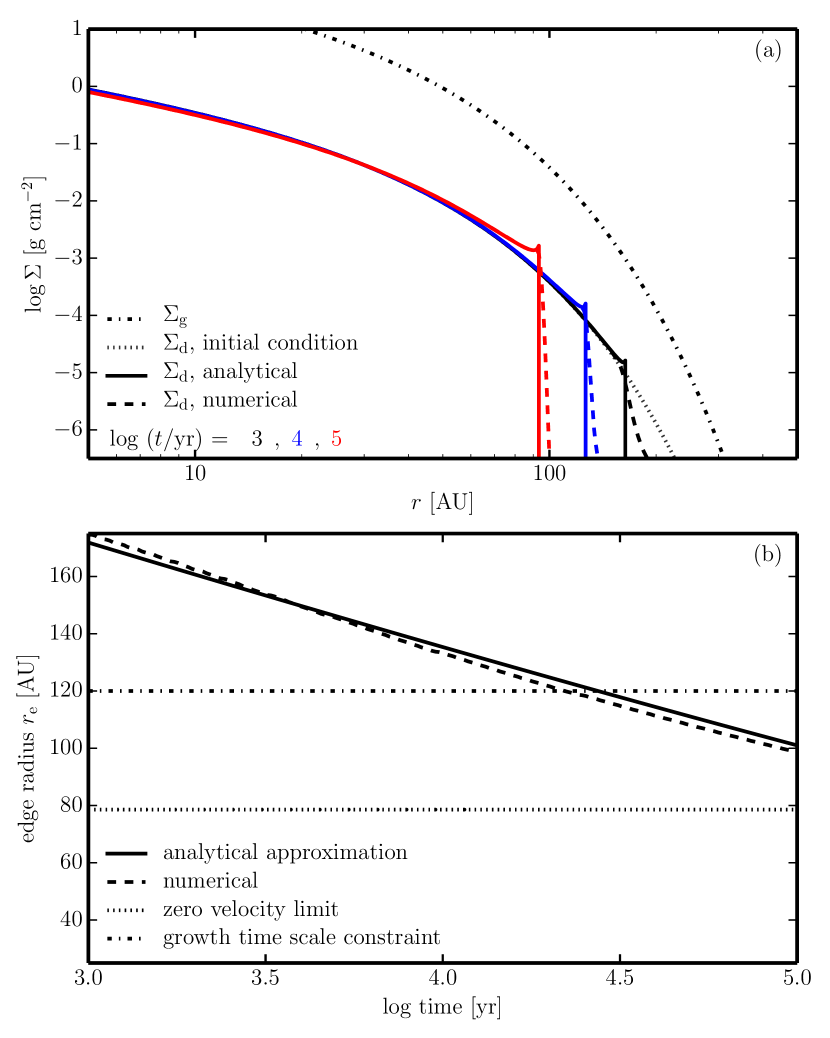
Figure 3.— (a) Analytical (solid) and numerical (dashed) calculations of the dust surface density evolution in the early phase as in Fig. 2, but in this case including gas drag. Note the enhancement of $\Sigma_{\mathrm{d}}$ near the dust edge, produced by the outward motion of dust entrained in the viscous gas flow. (b) The evolution of the outer dust edge including both radial drift and gas drag. In specific cases where the growth timescales (i.e., the duration of the early phase) are long or $\alpha_{\mathrm{t}}$ is high, the inward motion of the dust edge will be halted at a limiting radius where drift and drag are balanced (close to 80 AU in this case, see dotted line). Otherwise, the ultimate location of the dust edge will be set by the grain growth timescale ($\sim$120 AU for our parameters, cf. dash-dotted line).

The impact on $\Sigma_{\mathrm{d}}(r,t)$ and $r_{\mathrm{e}}(t)$ when gas drag and radial drift are incorporated together is described analytically in Appendix C and shown graphically in Figure 3. The outermost regions behave similarly to the drift-only case, since the $u_{\mathrm{rd}}$ term dominates at large $r$. However, just inside the dust edge there is a notable increase in $\Sigma_{\mathrm{d}}$ due to the outward motion of dust entrained in the viscous gas flow. Figure 1 demonstrates that this gas drag effect dominates the dust transport in a relatively narrow radial range. In essence, the outward-directed $u_{\mathrm{gd}}$ from the viscously expanding gas disk and the inward-directed $u_{\mathrm{rd}}$ converge near $r_{\mathrm{e}}$ and lead to a pile-up of dust.

The location of $r_{\mathrm{e}}$ shifts inward with time as in the drift-only case, but at some point the outward gas drag dominates and limits this evolution. This implies that the dust edge asymptotically approaches a minimum radius ($r_{\mathrm{e}}\geq r_{\mathrm{lim}}$) that can be estimated analytically,

$$\frac{r_{\mathrm{lim}}}{r_{\mathrm{c}}}=\mathcal{W}\left[\frac{3\,\alpha_{\mathrm{t}}}{\mathrm{St}_{0}}\,\exp\left(\frac{11}{4}\right)\right]-\frac{11}{4},$$ (10)

where we have used the Lambert $\mathcal{W}[\cdot]$ function (see Appendix C). The location of $r_{\mathrm{lim}}$, roughly 4 $r_{\mathrm{c}}$ (80 AU) in our fiducial model, is marked as a dotted line in the bottom panel of Figure 3. For our fiducial model, $r_{\mathrm{lim}}$ is well inside the limit to the inward motion of the dust edge imposed by the grain growth timescale constraint described above ($r_{\mathrm{e}}^{\mathrm{min}}$). But in principle, this drag-imposed limit on the dust edge location could be relevant in disks that are more turbulent (larger $\alpha_{\mathrm{t}}$) or have intrinsically longer growth timescales (e.g., brown dwarf disks).

To summarize, we have demonstrated analytically and numerically that the observational features noted in Section 1 — a sharp outer dust edge and corresponding decrease in the dust-to-gas ratio — are naturally generated by radial drift and, to a lesser extent gas drag, during an early phase in disk evolution, before substantial particle growth or viscous evolution have developed. In our fiducial example, the dust surface densities have decreased dramatically outside $\sim$5 $r_{\mathrm{c}}$ ($\sim$100 AU) within 0.1 Myr, before the grains have had a chance to grow beyond a few $\mu$m in size.

3. Late Phase

While the “early phase” discussed in the previous section represents a good approximation for dust transport in the outer disk, the dust in the inner disk is evolving very quickly and cannot be treated as if it has a fixed grain size. The particle size distribution and its associated velocities are time-dependent and spatially varying at smaller radii, and therefore the system is best studied with detailed numerical simulations (see Section 4). However, if particle growth has progressed to the point that it is limited by effects like fragmentation or the rapid removal of larger grains due to radial drift, we can define an analogous “late phase,” where particles have reached a maximum equilibrium size that depends on their distance to the host star. The timeframe where this late phase is valid depends intimately on the initial conditions and other parameters involved in the model, but a rough estimate of a few $\times$ $10^{5}$ years is a reasonable approximation.

3.1. Drift limited case

Birnstiel et al. (2012) showed that, if particles are not first subject to a barrier to their growth, the motion induced by radial drift itself imposes a size limit by removing large particles faster than collisional growth can replenish them. That limit is set to the size where the corresponding drift and growth timescales are roughly equal, and has an associated drift velocity

$$u_{\mathrm{rd}}=-f_{\mathrm{d}}\,S\,\epsilon\,V_{\mathrm{k}},$$ (11)

where the order-of-unity constant $f_{\mathrm{d}}$ was taken to be $0.3$. Comparing the drift limited transport velocity of Eq. 11 with the gas drag velocity, it can be shown that $u_{\mathrm{rd}}>u_{\mathrm{gd}}$ so long as $\epsilon\gtrsim 0.01\alpha_{\mathrm{t}}$.

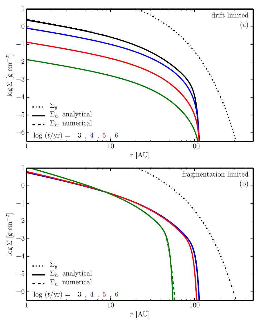
Figure 4.— The subsequent evolution of the dust surface density distribution during the “late phase,” when the maximum particle size is limited either by removal due to radial drift (a) or by grain fragmenting collisions (b). The notation is the same as in Figures 2 and 3.

We derive an analytic solution for $\Sigma_{\mathrm{d}}(r,t)$ in Appendix D, assuming that dust is transported with this drift limited velocity. The resulting behavior is shown in Figure 4(a), along with a comparison to the corresponding direct numerical calculations. Unlike in the early phase described in Section 2, drift according to Eq. 11 will not form a sharp outer edge by itself. Therefore, in this example, we have imposed an initial condition informed by the early phase results, such that the dust-to-gas ratio is constant in the inner disk ($\epsilon=10^{-2}$), but drops steeply beyond $r_{\mathrm{e}}\simeq 5~{}r_{\mathrm{c}}$. Figure 4(a) shows that the dust disk will effectively retain this shape: the location of the edge is fixed, but the drop-off in $\Sigma_{\mathrm{d}}$ gets progressively smoother as the dust mass homologously drains inward. The dust surface density in the inner disk is fed by the inward-drifting dust from the outer regions, and therefore follows the steady-state profile derived by Birnstiel et al. (2012): the radial power-law index of $\Sigma_{\mathrm{d}}$ (where $\Sigma\propto r^{-p}$) is $p_{\mathrm{d}}=(2\,p_{\mathrm{g}}+1)/4$, which for a local gas surface density index of $p_{\mathrm{g}}\simeq 1.2$ gives rise to $p_{\mathrm{d}}\simeq 0.85$, in agreement with the measured slope of 0.90 in Figure 5.

Transport along this radial drift barrier is self-regulating in the sense that the sizes particles can reach, and therefore also their drift speeds, depend on the dust-to-gas ratio, $\epsilon$. Consequently, a high $\epsilon$ produces fast drift motion and a rapid depletion of dust mass in the outer disk. Once $\epsilon$ is reduced as the disk evolves, particles are smaller and the decay of $\Sigma_{\mathrm{d}}$ proceeds more slowly. As can be seen from Eq. 11, the sticking efficiency, $S$, acts in the same way: if $S$ were 0.5 for the relevant grain sizes, then the drift timescales are twice as long, and the maximum sizes are twice as small.

3.2. Fragmentation limited case

A solution to the transport equations for the case where fragmentation limits the maximum grain sizes is derived in Appendix E. As for the drift limited case, no sharp outer edge is formed by this scenario itself. So, again, we impose an outer edge in the same way as the previous section, with an initial condition on $\epsilon(r)$ based on the calculations in Section 2. As long as there is still a significant outer disk that transports dust inwards, the inner regions in this scenario will generate a stationary $\Sigma_{\mathrm{d}}$ profile with a power-law index $p_{\mathrm{d}}\simeq 1.5$, as derived by Birnstiel et al. (2012).

The evolution of $\Sigma_{\mathrm{d}}$ in the fragmentation limited case, shown in Figure 4(b), is not self-regulating: particles drift at a constant rate that can be either fast or slow, depending on their size. Consequently, the outer dust edge moves inward as the disk evolves. If grain growth is limited by fragmentation, the edge can therefore be located substantially closer to the central stellar host.

4. Comparison to detailed simulations

We described above how dust transport processes in the “early” and “late” phases affect the dust surface density evolution in an analytic framework. However, to do this we had to make some important simplifications. In this section, we will compare this framework to a full suite of numerical simulations to test how well it describes the complicated behavior of a more realistic protoplanetary dust disk, where the constituent particles are growing and fragmenting upon collisions, migrating inwards due to radial drift, and at the same time being mixed and dragged along with the turbulent gas reservoir in which they are embedded. These detailed numerical simulations act as a reality check to test how well the adopted analytic simplifications hold, or whether neglected effects (e.g., particle size evolution, turbulent mixing) can cause significant deviations from the analytic results. The code used for these simulations was originally presented by Birnstiel et al. (2010). As initial conditions, we again assume a 0.8 $M_{\odot}$ stellar host, and adopt a $\Sigma_{\mathrm{g}}$ profile following Eq. 7, with an initial $r_{\mathrm{c}}=20$ AU, $\epsilon=0.01$ (at all $r$), $\alpha_{\mathrm{t}}=10^{-3}$, and disk mass of $0.01~{}M_{\odot}$. The initial particle size distribution was assumed to have a MRN-like slope, $n(a)\propto a^{-3.5}$, between 0.1 and 1 $\mu$m.

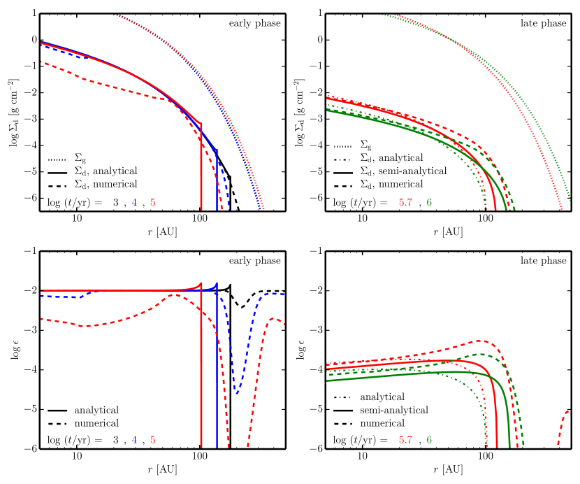
Figure 5.— A comparison between the predictions of the analytic framework (solid and dash-dotted) and the detailed numerical simulations (dashed) for the evolution of $\Sigma_{\mathrm{d}}$ (top) and $\epsilon$ (bottom) during the “early” and “late” phases (left and right, respectively). The snapshots correspond to $10^{3}$, $10^{4}$, and $10^{5}$ years in the early phase and to $5\times 10^{5}$, and $10^{6}$ years in the late phase. The simulations confirm that a sharp outer dust edge is formed quickly in both the analytic approximation and the numerical simulations, with deviations primarily related to the added sophistication of including particle growth and an initial distribution of particle sizes. The late phase in both cases are remarkably similar, considering the simplicity of the analytic approximation.

Figure 5 shows representative discrete steps in the evolutionary behavior of $\Sigma_{\mathrm{d}}(r,t)$ and $\epsilon(r,t)$ for the full numerical simulation, broken down into approximations of the “early” (left; $\lesssim$0.1 Myr) and “late” (right; $\gtrsim$0.1 Myr) phases to facilitate a direct comparison with the analytic prescriptions described in Sections 2 and 3, respectively, for the same initial conditions. Recall the discussion in Section 2.1 that showed how the analytical calculations for the early phase are only strictly valid for the radial range $\sim$120–280 AU. In the numerical simulations of the early phase, the dust-to-gas ratio in the inner disk deviates by about an order of magnitude from the analytic solution due to the onset of grain growth, an effect that was explicitly not treated in the simplified derivations of Section 2 (Appendix C). The numerical simulations also quickly form a sharp outer edge in the dust distribution at a similar location as predicted by the simple analytic solution, albeit with some differences in the details. The simulated edge is less sharp than the analytic prediction, partly due to real diffusion (because turbulent mixing is included in the simulations) but also due to numerical diffusion. Moreover, unlike the analytic solutions, the numerical code does not assume a monodisperse size distribution, but rather uses an MRN-like distribution, as an initial condition. Since each particle size is associated with a distinct outer edge location (cf., Eq. 10), a size distribution naturally produces a smoother edge. In this example, $\mu$m-sized grains have drifted further inward (to $\sim$100 AU) than the 0.1 $\mu$m-sized grains (which extend beyond 150 AU). Beyond $\sim$280 AU, the growth time scales again limit the applicability of the early phase solution (cf., Sect. 2.1), which explains the discrepancies at those distances. Despite these differences, it is clear that the fundamental prediction of the analytic models – that a relatively sharp edge in the dust distribution is formed quickly and maintained on longer timescales – is reproduced with good fidelity by the more sophisticated numerical simulations.

The right-hand panels of Figure 5 show the continued evolution of the disk in the “late” phase, where we have evolved the analytic result according to the drift limited scenario described in Appendix D (cf., dash-dotted curves). There are differences in the outer edge location in this comparison, stemming from the fact that the analytical drift solution does not include the viscous evolution of the gas disk. To remedy that, we included this effect in a semi-analytical way (see Appendix F): the results are shown in the right panels of Figure 5 as solid curves. There is remarkable agreement between the shape and overall absolute values of the surface densities between the numerical simulations and the semi-analytic results, especially considering the amount of simplification used to develop the latter. The semi-analytic results under-predict $\Sigma_{\mathrm{d}}$ in the outermost regions of the disk, partly because we neglected diffusion in that scenario, but mainly because the simple assumption that turbulence drives the collisional (and therefore growth) timescales (i.e., Eq. 1) becomes less accurate in the outer disk: at such low densities, drift-induced relative velocities become comparatively important (Birnstiel et al. 2012). In addition, our (semi-)analytical models used a mass-averaged size of 0.47 $\mu$m instead of the fixed assumption of 1 $\mu$m adopted in Section 2.1. A mass-averaged size is a good approximation in these calculations initially, however at later times the outer disk in the numerical simulation contains mostly smaller grains. This is why the viscous spreading of the outer edge proceeds further than in the analytical curves in Figure 5.

5. Discussion

We have developed an analytic framework that describes the bulk transport of solids embedded in a gas-rich, viscous accretion disk during two simplified evolutionary epochs. During an “early” phase in that evolution, before dust grains in the outer disk have had a chance to grow ($\lesssim$0.1 Myr), we find that the exponential taper in the gas surface densities beyond a characteristic radius ($r_{\mathrm{c}}$) substantially boosts the radial drift velocities for particles of any size. That inward migration naturally produces a sharp edge to the dust density distribution, or equivalently a steep drop in the dust-to-gas mass ratio, in the outer disk, representing a distinct and potentially observable “fingerprint” of the drift process. The location of this edge shifts inward with time, to a limit imposed by the grain growth timescale or viscous drag in the outward-spreading gas disk. While that location depends on detailed model parameters (particularly the grain size, gas surface density, and turbulence parameter), we expect typical edge radii of $\sim$3–8$\times$ the initial $r_{\mathrm{c}}$ (roughly 30–300 AU).

During a “late” phase of this evolution, once solid particles have grown larger (perhaps a few $\times 10^{5}$ yr), we solved the transport equations under the assumption that particle sizes are limited either by the drift or fragmentation barriers (cf., Birnstiel et al. 2012). Although the latter might be relevant initially, the decreasing dust-to-gas ratio will eventually ensure that drift is the barrier that limits particle growth in the outer disk. With this analytic prescription, we showed that the edge formed during the “early” phase is preserved, and its location does not change significantly (if the gas profile is fixed) or moves slightly outward (for a viscously spreading gas disk). A direct comparison to more sophisticated, time-dependent numerical simulations of the growth and transport of disk solids demonstrated that our simplified analytic framework faithfully captures the important features of the dust distribution in both the early and late phases.

That said, we should emphasize that this analysis does nothing to solve the “radial drift problem” (frequently termed the “m-size barrier”, although “mm/cm-size barrier” is more appropriate for the outer disk): there are still fundamental issues with the derived evolution timescales that are generally inconsistent with observations (e.g., Dominik et al. 2007; Brauer et al. 2007). One promising solution relies on pressure traps to stop or slow the radial drift of dust grains in the outer disk, generated either by turbulence or interactions with an embedded companion (e.g., Pinilla et al. 2012b, a). Note that traps of the right strength ($\mathrm{dln}{P}/\mathrm{dln}r\geq 0$) may present an alternative means of creating an outer edge in the dust distribution, for the same physical reasons outlined here.

The most fundamental (and perhaps obvious) conclusion from this study is that dust transport processes in a viscous accretion disk quickly modify the radial distribution of dust-to-gas ratios, $\epsilon(r)$, in the outer disk. Taking these calculations at face value, we must conclude that the typical assumption of $\Sigma_{\mathrm{d}}\propto\Sigma_{\mathrm{g}}$ in a protoplanetary disk is internally inconsistent. Therefore, the common practice of inferring $\Sigma_{\mathrm{d}}$ from observations based on a parametric prescription for a viscous gas disk (like Eq. 7; e.g., Andrews et al. 2009, 2010; Isella et al. 2009; Guilloteau et al. 2011) is not supported by any physical motivation. Instead, examination of the typical dust distributions derived from solving the transport equations suggests that a more reasonable parametric approximation for $\Sigma_{\mathrm{d}}(r)$ would be a multi-stage power-law with indices determined by the dust physics: $p_{\mathrm{d}}\simeq 1.5$ for a fragmentation-limited dust distribution in the inner disk, a smaller $p_{\mathrm{d}}$ for a drift-dominated dust distribution in the outer disk, and then a steep drop (large $p_{\mathrm{d}}$) outside of $r_{\mathrm{e}}$.

The key results from our dust transport calculations regarding the structural distributions of gas and solids in protoplanetary disks find strong, qualitative support from recent observations. A growing sample of disks have exhibited evidence for a size discrepancy in comparisons of their mm-wave emission in the CO line and associated continuum: the gas always appears more spatially extended than the dust (Panić et al. 2009; Andrews et al. 2012; de Gregorio-Monsalvo et al. 2013; Rosenfeld et al. 2013). Radiative transfer models confirm that this discrepancy is not an artifact of limited sensitivity, or optical depth effects. The dust transport calculations described here naturally reproduce this size discrepancy, due to the steep decrease in $\epsilon(r)$ near $r_{\mathrm{e}}$ created during the “early” phase of evolution. It is worth a reminder that, in the “late” phase, gas drag in the outward viscous flow can dominate drift velocities for small ($\mu$m-sized) particles that were originally confined inside $r_{\mathrm{e}}$ (indeed, this effect contributes to the smearing of the edge feature in the full numerical simulations presented in Section 4). This size-sorting offers a potential explanation for the spatial segregation of mm and $\mu$m-sized grains, where the latter appear in scattered light images to be more extended (e.g., compare Weinberger et al. 2002 and Andrews et al. 2012). Finally, very high quality mm-wave continuum emission measurements are starting to show the definitive signature of the sharp outer edge in the dust distribution that we have advocated, in the form of a distinctive oscillation pattern in their interferometric visibilities (Andrews et al. 2012; de Gregorio-Monsalvo et al. 2013).

The emerging consensus between observations and the theoretical framework developed here makes a strong case that dust transport dominated by radial drift plays a significant role in shaping the spatial distribution of disk solids. Ultimately, sensitive, high resolution mm-wave datasets should be able to place more quantitative constraints on this transport process. If observers continue to find sharp dust continuum edges and gas/dust size discrepancies in nearby disks, the combination of such measurements could in principle be linked to the key parameters $r_{\mathrm{e}}$ and $r_{\mathrm{c}}$, and thereby indirectly to $\epsilon(r)$ (which would help guide any revisions to transport simulations). Making a direct link between our simulations and observations is unfortunately complicated by the radial size-sorting that is also naturally imprinted by grain growth. While the total dust mass is confined within $r_{\mathrm{e}}$, the larger grains traced by radio interferometers are expected to be preferentially located at even smaller radii. In practice, some further development of our calculations and a link with radiative transfer models will be required to quantitatively aid the interpretation of mm/cm-wave continuum emission. With the start of science operations with the Atacama Large Millimeter/submillimeter Array (ALMA) and the recent upgrade of the Karl G. Jansky Very Large Array (VLA), the prospects are excellent for continued progress on this topic.

Appendix A A. General Solution

The general equation that describes the advective radial transport of the dust surface density in cylindrical coordinates is

$$\frac{\partial\Sigma_{\mathrm{d}}}{\partial t}+\frac{1}{r}\frac{\partial}{\partial r}\left(r\,u(r)\,\Sigma_{\mathrm{d}}\right)=0.$$ (A1)

Since the prescription we adopt to describe the gas surface densities is written in terms of the radius $r_{\mathrm{c}}$, it is convenient to introduce the dimensionless variable $x=r/r_{\mathrm{c}}$, such that

$$\frac{\partial\Sigma_{\mathrm{d}}}{\partial t}+\frac{1}{x}\frac{\partial}{\partial x}\left(\frac{x\,u(x)}{r_{\mathrm{c}}}\,\Sigma_{\mathrm{d}}\right)=0.$$ (A2)

The characteristic equations for this partial differential equation read

$$\frac{\mathrm{d}t}{\mathrm{d}s} = 1$$ (A3)

$$\frac{\mathrm{d}x}{\mathrm{d}s} = \frac{u(x)}{r_{\mathrm{c}}}$$ (A4)

$$\frac{\mathrm{d}\Sigma(s)}{\mathrm{d}s} = -\frac{\Sigma(s)}{r_{\mathrm{c}}\,x}\,\frac{\partial\left(u(x)\,x\right)}{\partial x}.$$ (A5)

The solution to Eq. A2 then can be written as

$$\Sigma(x,t)=\Sigma(x_{0},0)\,\frac{u(x_{0})\,x_{0}}{u(x)\,x},$$ (A6)

where $x_{0}$ is the position of the characteristic $s$ at dimensionless radius $x$ at time $t=0$, which is indirectly defined as

$$\frac{t}{r_{\mathrm{c}}}=\int_{x_{0}}^{x}\,\frac{1}{u(x^{\prime})}\,\mathrm{d}x^{\prime}.$$ (A7)

If the integral in Eq. A7 can be carried out and solved for $x_{0}$, the result represents the full, analytical solution to the advection equation. But even if this cannot be carried out analytically, a numerical evaluation of Eq. A7 is usually much faster than discretizing Eq. A1 and evolving it iteratively.

Appendix B B. Radial drift for a fixed particle size and $p_{\mathrm{gas}}=1$

In the following, we assume a time-independent gas surface density

$$\Sigma_{\mathrm{g}}(r)=\Sigma_{0}\,\left(\frac{r}{r_{\mathrm{c}}}\right)^{-p_{\mathrm{gas}}}\exp\left[-\left(\frac{r}{r_{\mathrm{c}}}\right)^{2-p_{\mathrm{gas}}}\right],$$ (B1)

where $p_{\mathrm{gas}}=1$ (as in Eq. 7) and a radial temperature dependence of

$$T(r)=T_{\mathrm{c}}\left(\frac{r}{r_{\mathrm{c}}}\right)^{-q},$$ (B2)

as in Eq. 7 and 8, respectively. In this structural parameterization and for a (radially) constant grain size without any growth, the dust drift velocity can be written as

$$u=-A\exp\left(x\right)\,x^{-q+3/2}\,\left(x+\frac{q+5}{2}\right),$$ (B3)

where

$$A=\frac{\mathrm{St}_{0}\,c_{\mathrm{c}}^{2}}{V_{\mathrm{c}}}$$ (B4)

(see Section 3.1 for symbol definitions). The system can be solved by numerically evaluating Eq. A7, however we can find a good approximation for large $x$ (the outer disk) using the velocity

$$u=-A\exp\left(x\right)\,x^{d},$$ (B5)

where $d=\frac{5}{2}-q$. With that approximation, Eq. A7 can be written

$$t(x,x_{0})=-\frac{r_{\mathrm{c}}}{A}\,\left(\Gamma\left[1-d,x_{0}\right]-\Gamma\left[1-d,x\right]\right),$$ (B6)

where $\Gamma(a,z)=\int_{z}^{\infty}t^{a-1}e^{-t}\,\mathrm{d}t$ is the incomplete gamma function. The approximate solution for the dust surface density evolution is therefore

$$\Sigma(x,t)=\Sigma(x_{0},0)\,\exp\left[-\left(x-x_{0}\right)\right]\,\left(\frac{x}{x_{0}}\right)^{-d-1}.$$ (B7)

For $x\gg 1$, we can replace the gamma function in Eq. B6 with $\Gamma(1-d,x)\simeq\exp(-x)\,x^{-d}$ and solve for $x_{0}$ to find

$$x_{0}=d\cdot\mathcal{W}\left[\frac{1}{d}\,\left(\mathrm{e}^{-x}\,x^{-d}-\frac{A\,t}{r_{\mathrm{c}}}\right)^{-1/d}\right],$$ (B8)

where $\mathcal{W}\left[\cdot\right]$ is the Lambert $\mathcal{W}$-function, also known as product logarithm or omega function (note that the $\mathcal{W}$ function is readily available in most mathematical software).

Eq. B7 together with Eq. B8 provides a good approximate solution to the transport equation. There exists a location $x_{\mathrm{e}}$ where $x_{0}$ diverges, meaning that all $x_{0}$ outside $x_{\mathrm{e}}$ have moved inward of this point (i.e., $x_{\mathrm{e}}$ represents the outer edge of the dust disk). This edge location is approximately

$$x_{\mathrm{e}}=\frac{r_{\mathrm{e}}}{r_{\mathrm{c}}}=d\cdot\mathcal{W}\left[\frac{1}{d}\left(\frac{A\,t}{r_{\mathrm{c}}}\right)^{-1/d}\right].$$ (B9)

Appendix C C. Including gas drag

If we include the gas drag velocity, Eq. 3, for $p_{\mathrm{gas}}=1$ and $q=\frac{1}{2}$, we get a velocity of

$$u=B\,\left(x-\frac{1}{2}\right)-A\,x\,\exp(x)\left(x+\frac{11}{4}\right),$$ (C1)

where $B=3\alpha_{\mathrm{t}}\,c_{\mathrm{c}}^{2}/V_{\mathrm{c}}$. The solution to the advection equation is then given by

$$\Sigma_{\mathrm{d}}(x,t)=\Sigma_{\mathrm{d}}(x_{0},0)\frac{x_{0}}{x}\frac{x_{0}-\frac{1}{2}-\mathrm{Pe}_{0}\,x_{0}\,\exp(x_{0})\,\left(x_{0}+11/4\right)}{x-\frac{1}{2}-\mathrm{Pe}_{0}\,x\,\exp(x)\,\left(x+11/4\right)},$$ (C2)

where $\mathrm{Pe}_{0}=\mathrm{\mathrm{St}_{0}}/3\alpha_{\mathrm{t}}$ ($\simeq$ the Péclet number) and $x_{0}$ is defined by

$$t=r_{\mathrm{c}}\int_{x_{0}}^{x}\left(B\,\left(x^{\prime}-\frac{1}{2}\right)-A\,x^{\prime}\,\exp(x^{\prime})\,\left(x^{\prime}+\frac{11}{4}\right)\right)^{-1}\mathrm{d}x^{\prime}.$$ (C3)

Appendix D D. Drift-limited Solution

The velocity of particles in the drift-limited scenario (see Birnstiel et al. 2012) is given by

$$u=-f_{\mathrm{d}}\,S\,\epsilon\,V_{\mathrm{k}},$$ (D1)

where $\epsilon=\Sigma_{\mathrm{d}}/\Sigma_{\mathrm{g}}$, implying that, in contrast to above, the velocity is now a function of both position and $\Sigma_{\mathrm{d}}$. Analogous to the derivation in Appendix A, the characteristic equations become

$$s = f_{\mathrm{d}}\,S\,t$$ (D2)

$$\frac{\mathrm{d}r}{\mathrm{d}s} = -2\,\epsilon\,V_{\mathrm{k}}$$ (D3)

$$\frac{\mathrm{d}\Sigma_{\mathrm{d}}}{\mathrm{d}s} = \frac{\Sigma_{\mathrm{d}}^{2}}{\Sigma_{\mathrm{g}}}\,\Omega_{\mathrm{k}}+\Sigma_{\mathrm{d}}^{2}\,\frac{\mathrm{d}}{\mathrm{d}r}\left(\frac{V_{\mathrm{k}}}{\Sigma_{\mathrm{g}}}\right)$$ (D4)

and yield the solution

$$\Sigma_{\mathrm{d}}(x,t)=\Sigma_{\mathrm{d}}(x_{0},0)\,\left(\frac{x}{x_{0}}\right)^{-1/4}\,\left(\frac{\Sigma_{\mathrm{g}}(x)}{\Sigma_{\mathrm{g}}(x_{0})}\right)^{1/2},$$ (D5)

where $x_{0}$ is again the initial position of a test particle, such that

$$t=-\frac{r_{\mathrm{c}}\,\sqrt{\Sigma_{\mathrm{g}}(x_{0})}}{2f_{\mathrm{d}}\,S\,V_{\mathrm{c}}\,x_{0}^{1/4}\,\Sigma_{\mathrm{d}}(x_{0},0)}\,\int_{x_{0}}^{x}{x^{\prime}}^{3/4}\,\Sigma_{\mathrm{g}}(x^{\prime})^{1/2}\,\mathrm{d}x^{\prime}.$$ (D6)

For the gas surface density profile as in Eq. B1 with $p_{\mathrm{gas}}=1$ or also for a slightly more general case of

$$\Sigma_{\mathrm{g}}(r)=\Sigma_{0}\,\left(\frac{r}{r_{\mathrm{c}}}\right)^{-p_{\mathrm{gas}}}\exp\left[-\frac{r}{r_{\mathrm{c}}}\right],$$ (D7)

and $p_{\mathrm{gas}}<7/2$, $x_{0}$ is the solution to

$$t(x,x_{0})=\frac{\Sigma_{0}\,r_{\mathrm{c}}\,2^{(3-2\,p_{\mathrm{gas}})/4}\,\exp\left[-x_{0}/2\right]}{f_{\mathrm{d}}\,S\,\Sigma_{\mathrm{d}}(x_{0},0)\,V_{\mathrm{c}}\,x_{0}^{(2\,p_{\mathrm{gas}}+1)/4}}\,\left(\Gamma\left[\frac{7-2\,p_{\mathrm{gas}}}{4},\frac{x}{2}\right]-\Gamma\left[\frac{7-2\,p_{\mathrm{gas}}}{4},\frac{x_{0}}{2}\right]\right),$$ (D8)

which needs to be solved numerically. We can find approximate solutions for $x_{0}$ by approximating the gamma function as before. In the case of $x_{0},x\gg 1$, Eq. D8 yields

$$x_{0}=\frac{1}{2}\,\mathcal{W}\left[2\left(f_{\mathrm{d}}\,S\,\epsilon\,\Omega_{\mathrm{c}}\,t\right)^{4}\frac{\exp(x)}{x}\right],$$ (D9)

where $\Omega_{\mathrm{c}}$ is the Keplerian frequency at $r_{\mathrm{c}}$. Eq. D5 also holds for a gas surface density profile

$$\Sigma_{\mathrm{g}}(r)=\Sigma_{\mathrm{c}}\,\left(\frac{r}{r_{\mathrm{c}}}\right)^{-p_{\mathrm{gas}}},$$ (D10)

in which case $r_{0}$ is the solution of

$$t=\frac{2}{7-2\,p_{\mathrm{gas}}}\frac{\Sigma_{\mathrm{c}}\,r_{0}}{f_{\mathrm{d}}\,S\,\Sigma_{\mathrm{d}}(r_{0},0)\,V_{\mathrm{k}}(r_{0})}\,\left(\frac{r_{0}}{r_{\mathrm{c}}}\right)^{-p_{\mathrm{gas}}}\,\left[1-\left(\frac{r}{r_{0}}\right)^{(7-2\,p_{\mathrm{gas}})/4}\right].$$ (D11)

Appendix E E. Fragmentation-limited Solution

The Stokes number in the fragmentation-limited case (i.e., when the maximum impact velocity exceeds the fragmentation velocity, $u_{\mathrm{frag}}\lesssim\sqrt{\alpha_{\mathrm{t}}}\,c_{\mathrm{s}}$) can be approximated as

$$\mathrm{St}\simeq\frac{1}{3\,\alpha_{\mathrm{t}}}\,\frac{u_{\mathrm{frag}}^{2}}{c_{\mathrm{s}}^{2}},$$ (E1)

which gives a drift velocity of

$$u\simeq-B\sqrt{x}\left(x+\frac{q+5}{2}\right),$$ (E2)

with $B=f_{\mathrm{f}}\,u_{\mathrm{frag}}^{2}/3\alpha_{\mathrm{t}}\,V_{\mathrm{c}}$ and $f_{\mathrm{f}}=0.37$ (see Birnstiel et al. 2012). Using this velocity in Eq. A7, we can derive the solution for $x_{0}$ to be

$$x_{0}=\frac{q+5}{2}\,\left\{\tan\left[\frac{B}{2}\sqrt{\frac{q+5}{2}}\frac{t}{r_{\mathrm{c}}}-\arctan\left(\sqrt{\frac{q+5}{2\,x}}\right)\right]\right\}^{-2},$$ (E3)

which, used in Eq. A6, describes the time evolution of $\Sigma_{\mathrm{d}}$ in the fragmentation-limited case.

Appendix F F. Advection of a tracer in a viscously evolving accretion disk

Quite similar to before (cf., Eq. B1 and assuming $p_{\mathrm{gas}}=1$), the time dependent gas surface density can be written as

$$\Sigma_{\mathrm{g}}(r,t)=\Sigma_{0}(t)\,\left(\frac{r}{r_{\mathrm{c}}(t)}\right)^{-1}\exp\left(-\frac{r}{r_{\mathrm{c}}(t)}\right),$$ (F1)

however the characteristic radius and the normalization are now time dependent,

$$\Sigma_{0}(t)=\frac{C}{3\pi\nu_{1}}\,\left(\frac{r_{\mathrm{c}}(t)}{r_{1}}\right)^{-5/2},$$ (F2)

and

$$r_{\mathrm{c}}(t)=r_{1}+\frac{3\,t\,\nu_{1}}{r_{1}},$$ (F3)

as can be derived from Hartmann et al. (1998) or Lynden-Bell & Pringle (1974). $C$ is a constant normalization factor proportional to the initial disk mass. The gas velocity then also becomes time-dependent,

$$u_{\mathrm{gas}}(r,t)=\frac{3\nu_{1}}{r_{1}}\left(\frac{r}{r_{\mathrm{c}}(t)}-\frac{1}{2}\right),$$ (F4)

and we assumed the viscosity to follow $\nu=\nu_{1}\cdot(r/r_{1}$). Small particles with $\mathrm{St}\ll 1$ then move with the gas radial velocity, and the time evolution can be solved for using characteristics as before, yielding

$$\Sigma_{\mathrm{d}}(r,t)=\Sigma_{\mathrm{d}}(r_{i},0)\cdot\left[\left(\frac{r_{\mathrm{c}}(t)}{r_{1}}\right)^{2}\,\left(1+\frac{1}{2}\,\frac{r_{1}}{r_{i}}\log\left(\frac{r_{1}}{r_{\mathrm{c}}(t)}\right)\right)\right]^{-1},$$ (F5)

where the initial position of a characteristic is defined to be

$$r_{i}(r,t)=\frac{r_{1}}{2}\cdot\left[\ln\left(\frac{r_{\mathrm{c}}(t)}{r_{1}}\right)+2\,\frac{r}{r_{\mathrm{c}}(t)}\right].$$ (F6)

To semi-analytically calculate the evolution of $\Sigma_{\mathrm{d}}$ when both radial drift (according to Appendix D) and viscous spreading are taken into account, we iterated between these two analytical solutions:

1. choose a time step $\Delta t$ within which the gas surface density does not change dramatically

2. calculate how the dust is advected along with the gas according Eq. F5 during $\Delta t$

3. use the result from (2) as an initial condition for Eq. D5 using the same time step

4. continue with step 1

The results shown in Fig. 5 were derived using nine logarithmically spaced time steps between $10^{5}$ and $10^{6}$ years.

References

- Allen et al. (2001) Allen, R. L., Bernstein, G. M., & Malhotra, R. 2001, ApJ, 549, L241
- Andrews et al. (2009) Andrews, S. M., Wilner, D. J., Hughes, A. M., Qi, C., & Dullemond, C. P. 2009, ApJ, 700, 1502
- Andrews et al. (2010) Andrews, S. M., Wilner, D. J., Hughes, A. M., Qi, C., & Dullemond, C. P. 2010, ApJ, 723, 1241
- Andrews et al. (2012) Andrews, S. M., Wilner, D. J., Hughes, A. M., et al. 2012, ApJ, 744, 162
- Beckwith & Sargent (1993) Beckwith, S. V. W. & Sargent, A. I. 1993, ApJ, 402, 280
- Beckwith et al. (1990) Beckwith, S. V. W., Sargent, A. I., Chini, R. S., & Guesten, R. 1990, AJ, 99, 924
- Birnstiel et al. (2010) Birnstiel, T., Dullemond, C. P., & Brauer, F. 2010, A&A, 513, 79
- Birnstiel et al. (2012) Birnstiel, T., Klahr, H., & Ercolano, B. 2012, A&A, 539, 148
- Birnstiel et al. (2011) Birnstiel, T., Ormel, C. W., & Dullemond, C. P. 2011, A&A, 525, 11
- Brauer et al. (2008) Brauer, F., Dullemond, C. P., & Henning, T. 2008, A&A, 480, 859
- Brauer et al. (2007) Brauer, F., Dullemond, C. P., Johansen, A., et al. 2007, A&A, 469, 1169
- de Gregorio-Monsalvo et al. (2013) de Gregorio-Monsalvo, I., Ménard, F., Dent, W., et al. 2013, A&A, 557, 133
- Dominik et al. (2007) Dominik, C., Blum, J., Cuzzi, J. N., & Wurm, G. 2007, PP V, 783
- Dutrey et al. (1998) Dutrey, A., Guilloteau, S., Prato, L., et al. 1998, A&A, 338, L63
- Guilloteau & Dutrey (1998) Guilloteau, S. & Dutrey, A. 1998, A&A, 339, 467
- Guilloteau et al. (2011) Guilloteau, S., Dutrey, A., Piétu, V., & Boehler, Y. 2011, A&A, 529, 105
- Hartmann et al. (1998) Hartmann, L., Calvet, N., Gullbring, E., & D’Alessio, P. 1998, ApJ, 495, 385
- Hughes et al. (2008) Hughes, A. M., Wilner, D. J., Qi, C., & Hogerheijde, M. R. 2008, ApJ, 678, 1119
- Isella et al. (2009) Isella, A., Carpenter, J. M., & Sargent, A. I. 2009, ApJ, 701, 260
- Isella et al. (2007) Isella, A., Testi, L., Natta, A., et al. 2007, A&A, 469, 213
- Jacquet et al. (2012) Jacquet, E., Gounelle, M., & Fromang, S. 2012, Icarus, 220, 162
- Jewitt et al. (1998) Jewitt, D., Luu, J., & Trujillo, C. 1998, AJ, 115, 2125
- Kornet et al. (2001) Kornet, K., Stepinski, T. F., & Różyczka, M. 2001, A&A, 378, 180
- Lynden-Bell & Pringle (1974) Lynden-Bell, D. & Pringle, J. E. 1974, MNRAS, 168, 603
- Mathis et al. (1977) Mathis, J. S., Rumpl, W., & Nordsieck, K. H. 1977, ApJ, 217, 425
- Nakagawa et al. (1986) Nakagawa, Y., Sekiya, M., & Hayashi, C. 1986, Icarus, 67, 375
- Ormel & Cuzzi (2007) Ormel, C. W. & Cuzzi, J. N. 2007, A&A, 466, 413
- Ossenkopf & Henning (1994) Ossenkopf, V. & Henning, T. 1994, A&A, 291, 943
- Panić et al. (2009) Panić, O., Hogerheijde, M. R., Wilner, D., & Qi, C. 2009, A&A, 501, 269
- Piétu et al. (2007) Piétu, V., Dutrey, A., & Guilloteau, S. 2007, A&A, 467, 163
- Piétu et al. (2005) Piétu, V., Guilloteau, S., & Dutrey, A. 2005, A&A, 443, 945
- Pinilla et al. (2012a) Pinilla, P., Benisty, M., & Birnstiel, T. 2012a, A&A, 545, 81
- Pinilla et al. (2012b) Pinilla, P., Birnstiel, T., Ricci, L., et al. 2012b, A&A, 538, 114
- Rosenfeld et al. (2013) Rosenfeld, K. A., Andrews, S. M., Hughes, A. M., Wilner, D. J., & Qi, C. 2013, ApJ, 774, 16
- Shakura & Sunyaev (1973) Shakura, N. I. & Sunyaev, R. A. 1973, A&A, 24, 337
- Tanaka et al. (1996) Tanaka, H., Inaba, S., & Nakazawa, K. 1996, Icarus, 123, 450
- Trujillo et al. (2001) Trujillo, C. A., Jewitt, D. C., & Luu, J. X. 2001, AJ, 122, 457
- Weidenschilling (2003) Weidenschilling, S. J. 2003, Lunar Planet. Sci., 34, 1707
- Weinberger et al. (2002) Weinberger, A. J., Becklin, E. E., Schneider, G., et al. 2002, ApJ, 566, 409
- Youdin & Shu (2002) Youdin, A. N. & Shu, F. H. 2002, ApJ, 580, 494