Convergence Tools for Consensus in Multi-Agent Systems with Switching Topologies

Abstract

We present two main theorems along the lines of Lyapunov’s second method that guarantee asymptotic state consensus in multi-agent systems of agents in $\mathbb{R}^{m}$ with switching interconnection topologies. The two theorems complement each other in the sense that the first one is formulated in terms of the states of the agents in the multi-agent system, whereas the second one is formulated in terms of the pairwise states for each pair of agents in the multi-agent system. In the first theorem, under the assumption that the interconnection topology is uniformly strongly connected and that the agents are contained in a compact set, a strong form of attractiveness of the consensus set is assured. In the second theorem, under the weaker assumption that the interconnection topology is uniformly quasi strongly connected, the consensus set is guaranteed to be uniformly asymptotically stable.

,

1 Introduction

The field of networked and multi-agent systems has received growing interest from researchers within robotics and control theory during the last decade [16]. This increased attention to network science is partly due to the recent advancement of communication technologies such as cellular phones, the Internet, GPS, wireless sensor networks etc. The widespread use and ongoing development of such technologies is a testament to the great potential applicability of the work carried out within this research field.

Consensus is a key problem in multi-agent systems theory and it has indeed also been one of the main objects of attention. Early works include [27, 31]. Some of the most well cited publications within the control community are [20, 22, 21, 24]. Due to the vast amount of publications, it is a challenge to provide a complete overview of the subject, and in this introduction we merely provide a selection from the body of knowledge. There are books [16, 26], and surveys [8, 25] covering the subject from different perspectives.

The problem of consensus or state agreement can roughly be explained as follows. Given a multi-agent system where each agent has a state in a common space and where the states are updated to a dynamical equation, design a distributed control law for the system such that the states of the agents converge to the same value. The convergence is mostly defined in the asymptotic sense.

The dynamics for the agents can either be described in discrete time [17, 32] or continuous time [19]. This work considers continuous time dynamics. Furthermore, if the dynamics is linear, much of the work has centered around graph theoretic concepts such as the graph Laplacian matrix, and its importance for the convergence to the consensus manifold [16, 23, 22]. For homogeneous systems of agents with linear dynamics, the question of which properties must hold in order to guarantee consensus has been answered [14].

Here, similar to [13, 20, 29], we consider a broad class of multi-agent systems and provide some criteria in order to guarantee consensus which are common for a class of systems. In those works, consensus is assured by imposing a convexity assumption. Roughly, provided the existence and uniqueness of solution is guaranteed, if the right-hand side of each agent’s dynamics, is inward-pointing [2] relative to the convex hull of the position of itself and the positions of its neighbors (states), asymptotic consensus is guaranteed.

Instead of using a convexity assumption, in this work we provide two classes of functions. Provided certain conditions are fulfilled for the system and the functions, two theorems guarantee consensus or state agreement. The first class of functions are functions of state, and the second class of functions are functions of pairs of states. The two theorems differ in the sense that the first one is formulated for functions in the first class and the second one is formulated for functions in the second class. The theorems can be combined in order to show consensus under the convexity assumptions in [13, 20, 29]. However, as we show, there are examples when the convexity assumptions do not hold but where the proposed theorems can be applied.

The proposed functions can be interpreted as Lyapunov-like functions in order to show consensus for multi-agent systems. If a function is used from the first class, a strong form of attractiveness of the consensus set is shown in the first theorem. On the contrary, if a function from the second class is used, uniform asymptotic stability to the consensus manifold is shown in the second theorem. Even though the second theorem provides stronger conditions for convergence, the first theorem can in general be applied in wider context.

We provide numerous examples of the usefulness of the theorems. One such example regards nonlinear scaling in a well known consensus control law for agents with single integrator dynamics. This control law consists of a weighted sum of the pairwise differences between neighboring agents. In the modified nonlinear scaled version, either the states have been scaled, or the differences between the states have been scaled. If the differences have been scaled, the control law falls into the frameworks of [13, 20, 29]. However, if the states are scaled, this situation is not captured by the convexity assumption, but the first theorem we present is still applicable.

Connectivity is key to achieving collective behavior in a multi-agent system. In fact, the topologies for the practical multi-agent networks may change over time. In the study of variable topologies, a well-known connectivity assumption, called (uniform) joint connection without requiring connectedness of the graph at every moment, was employed to guarantee multi-agent consensus for first-order or second-order linear or nonlinear systems [5, 10, 11, 29].

Under these mild switching conditions we allow the right-hand side of the system dynamics to switch between a finite set of functions that are piecewise continuous in the time and uniformly Lipschitz in the state on some compact region containing the origin. Similar to earlier works we assume a positive lower bound on the dwell time between two consecutive time instances where the right-hand side switches between two functions in the set. Also we require in general an upper bound on the dwell time (in the case of time invariant functions we do not require such an upper bound).

The time dependence in the right-hand side of the system dynamics is restricted in the sense that it only depends on the time since the last switch between two functions. This type of time dependence can be used in a wide range of applications, for example one can show that for a system switching between a finite set of time invariant functions, one can define continuous in time transitions between the functions instead of discontinuous switches, so that the right-hand side of the system dynamics is continuous and the system reaches consensus with the same rate of convergence as for the switching system.

2 Preliminaries

2.1 Dynamics

Let us introduce the following finite set of functions

$$\mathcal{F}=\{\tilde{f}_{1}(t,x),\ldots,\tilde{f}_{|\mathcal{F}|}(t,x)\},$$

where

$$\tilde{f}_{k}:\mathbb{R}\times\mathbb{R}^{mn}\rightarrow\mathbb{R}^{mn},\text{ for all }k=\{1,\ldots,|\mathcal{F}|\},$$

is continuous in $t$ and Lipschitz in $x$, uniformly with respect to $t$, on some open connected set containing the compact region $\mathcal{D}\in\mathbb{R}^{mn}$. We assume that $\mathcal{D}$ contains the origin as an interior point. The symbol $|\mathcal{F}|$ is the number of functions in $\mathcal{F}$. Each function $\tilde{f}_{k}\in\mathcal{F}$ can be written as $\tilde{f}_{k}=(\tilde{f}_{k,1},\ldots,\tilde{f}_{k,n})^{T}$, where

$$\tilde{f}_{k,l}:\mathbb{R}\times\mathbb{R}^{mn}\rightarrow\mathbb{R}^{m}\quad\text{ for all }\>l.$$

By following [5], we define switching signal functions which will be used in the definition of the system dynamics. We will assume that a switching signal function $\sigma$ satisfies either Assumption 2.1 (1,2) or Assumption 2.1 (1,2,3) below (what we mean by e.g., (1,2) is that the conditions 1 and 2 are satisfied).

Assumption .

1. The function $\sigma(t):\mathbb{R}\rightarrow\{1,\ldots,|\mathcal{F}|\}$ is piecewise right-continuous.
   

2. There is a monotonically increasing sequence $\{\tau_{k}\}$, such that $\tau_{k}\rightarrow\infty$ as $k\rightarrow\infty$ and $\tau_{k}\rightarrow-\infty$ as $k\rightarrow-\infty$, where each $\tau_{k}\in\mathbb{R}$ is such that for any $k\in\mathbb{Z}$ the function $\sigma$ is constant on $[\tau_{k},\tau_{k+1})$ for all $k$, and there is a $\tau_{D}>0$ such that

   $$\inf_{k}(\tau_{k+1}-\tau_{k})\geq\tau_{D}\text{ and }$$

3. there is an upper bound $\tau_{U}>0$, such that for any

   $$\sup_{k}(\tau_{k+1}-\tau_{k})\leq\tau_{U}.\quad$$

We define the set of all functions $\sigma$ that fulfills Assumption 2.1 (1,2) as $\mathcal{S}_{|\mathcal{F}|,D}$ and fulfills Assumption 2.1 (1,2,3) as $\mathcal{S}_{|\mathcal{F}|,D,U}$. The constants $\tau_{D}$ and $\tau_{U}$ might be different for different $\sigma$, so condition 2 and 3 in Assumption 2.1 can also be formulated as

$$\inf_{k}(\tau_{k+1}-\tau_{k})>0\quad\text{ and }\quad\sup_{k}(\tau_{k+1}-\tau_{k})<\infty$$

respectively. For each $\sigma$, the sequence $\{\tau_{k}\}$ is referred to as the switching times of $\sigma$, since it is only at those times $\sigma(t)$ changes value. If we compare the upper and lower bounds for two switching signal functions $\sigma_{1}$ and $\sigma_{2}$, we denote the upper and lower bound for $\sigma_{1}$ as $\tau_{U}^{\sigma_{1}}$ and $\tau_{D}^{\sigma_{1}}$ respectively and the upper and lower bound for $\sigma_{2}$ as $\tau_{U}^{\sigma_{2}}$ and $\tau_{D}^{\sigma_{2}}$ respectively.

For a given $\sigma\in\mathcal{S}_{|\mathcal{F}|,D}$ with switching times $\{\tau_{k}\}$ we define (for finite times)

$$\gamma_{\sigma}(t)=\max\{\tau_{k}:\tau_{k}\leq t,k\in\mathbb{Z}\},$$

where $\gamma_{\sigma}(t)$ is the largest switching time less than or equal to $t$.

Let us now consider a system of $n$ agents. The state of agent $i$ at time $t$ is defined as $x_{i}(t)\in\mathbb{R}^{m}$. The dynamics for the system of agents that we consider is given by

$$\dot{x}_{1}= ~{}f_{1}(t,x)=\tilde{f}_{\sigma(t),1}(t-\gamma_{\sigma}(t),x),$$

$$\vdots\>$$

$$\dot{x}_{n}= ~{}f_{n}(t,x)=\tilde{f}_{\sigma(t),n}(t-\gamma_{\sigma}(t),x),$$

where $\sigma\in\mathcal{S}_{|\mathcal{F}|,D}$ and

$$(\tilde{f}_{\sigma(t),1},\ldots,\tilde{f}_{\sigma(t),n})^{T}=\tilde{f}_{\sigma(t)}\in\mathcal{F}.$$

Note that $f_{i}(t,x)\in\mathbb{R}^{m}$ for $i\in\{1,\ldots,n\}$, whereas $\tilde{f}_{i}(t,x)\in\mathbb{R}^{mn}$ for $i\in\{1,\ldots,|\mathcal{F}|\}$. The main results in this work regard the restricted case when $\sigma\in\mathcal{S}_{|\mathcal{F}|,D,U}$, however there are cases when we assume the general case when $\sigma\in\mathcal{S}_{|\mathcal{F}|,D}$. The system dynamics can be written as

$$\dot{x}=f(t,x)=\tilde{f}_{\sigma(t)}(t-\gamma_{\sigma}(t),x),$$ (1)

where, $f(t,x)=\>(f_{1}(t,x),\ldots,f_{n}(t,x))^{T}.$ For a given $\sigma$, the function $f(t,x)$ is piecewise continuous in $t$. It is Lipschitz in $x$ on $\mathcal{D}$, uniformly with respect to $t$. The initial state and the initial time for (1) is $x_{0}\in\mathcal{D}$ and $t_{0}$ respectively. Sometimes we write $x(t_{0})$ instead of $x_{0}$.

The switching signal functions are used in order to indicate which system we are referring to. For a given $\mathcal{F}$, the switching behavior of the system is captured by $\sigma$. In order to emphasize this, instead of writing $x$ we can write

$$x^{\sigma}=(x^{\sigma}_{1},\ldots,x^{\sigma}_{n})^{T}.$$

In general we omit the parametrization by $\sigma$ and write $x$ instead of $x^{\sigma}$, but the latter notation is useful when we study solutions of (1) for different choices of $\sigma$. The solution for the system (1) is sometimes also written as $x(t,t_{0},x_{0})$ or $x^{\sigma}(t,t_{0},x_{0})$, where the explicit dependence on the initial time $t_{0}$ and the initial state $x_{0}$ is emphasized.

Lemma .

If all the functions in $\mathcal{F}$ are time-invariant, the dynamics (1) is given by

$$\dot{x}=\tilde{f}_{\sigma(t)}(x),$$

and if $\sigma\in\mathcal{S}_{|\mathcal{F}|,D}$ but $\sigma\not\in\mathcal{S}_{|\mathcal{F}|,D,U}$, it holds that there is a corresponding $\sigma^{\prime}\in\mathcal{S}_{|\mathcal{F}|,D,U}$ for which the dynamics is the same. i.e.,

$$\dot{x}=\tilde{f}_{\sigma^{\prime}(t)}(x)=\tilde{f}_{\sigma(t)}(x)$$

for all $t\geq 0$.

Lemma .

For $\sigma\in\mathcal{S}_{|\mathcal{F}|,D,U}$ with lower bound $\tau_{D}^{\sigma}$ and upper bound $\tau_{U}^{\sigma}$ on the dwell time between two consecutive switches, there is a finite set of functions (continuous in $t$ and Lipschitz in $x$ on $\mathcal{D}$, uniformly with respect to $t$)

$$\mathcal{F}^{\prime}=\{\tilde{f}_{1}^{\prime},\ldots,\tilde{f}_{|\mathcal{F}^{\prime}|}^{\prime}\}\supset\mathcal{F}$$

and $\sigma^{\prime}\in\mathcal{S}_{|\mathcal{F}^{\prime}|,D,U}$ with a lower bound $\tau_{D}^{\sigma^{\prime}}=\tau_{D}^{\sigma}$ and an upper bound $\tau_{U}^{\sigma^{\prime}}=2\tau_{D}^{\sigma}$ on the dwell time between two consecutive switches, such that

$$\tilde{f}^{\prime}_{\sigma^{\prime}(t)}(t-\gamma_{\sigma^{\prime}}(t),x)=\tilde{f}_{\sigma(t)}(t-\gamma_{\sigma}(t),x).$$

The proofs of these lemmas as well as all other proofs that are not given directly are contained in Section 5. Due to Lemma 2.1, we will often consider the case when $\tau_{U}=2\tau_{D}$ since we can replace $\mathcal{F}$ with $\mathcal{F}^{\prime}$ and $\sigma$ with $\sigma^{\prime}$. Note that $\tau_{D}^{\sigma}$ and $\tau_{U}^{\sigma}$ do not need to be the greatest lower bound and the least upper bound respectively for the dwell time between two consecutive switches of $\sigma$.

2.2 Connectivity

In a multi-agent system the dynamical behavior in general depends on the connectivity between the agents. The connectivity is described by a graph.

Definition .

A directed graph (or digraph) $\mathcal{G}=(\mathcal{V},\mathcal{E})$ consists of a set of nodes, $\mathcal{V}=\{1,...,n\}$ and a set of edges $\mathcal{E}\subset\mathcal{V}\times\mathcal{V}$.

In our setting, each node in the graph corresponds to a unique agent. Thus $\mathcal{V}$ is henceforth defined as $\mathcal{V}=\{1,...,n\}$. We also define neighbor sets or neighborhoods. Let $\mathcal{N}_{i}\in\mathcal{V}$ comprise the neighbor set (sometimes referred to simply as neighbors) of agent $i$, where $j\in\mathcal{N}_{i}$ if and only if $(j,i)\in\mathcal{E}$. We assume throughout the thesis that $i\in\mathcal{N}_{i}$ i.e., we restrict the collection of graphs to those for which $(i,i)\in\mathcal{E}$ for all $i\in\mathcal{V}$.

A directed path of $\mathcal{G}$ is an ordered sequence of distinct nodes in $\mathcal{V}$ such that any consecutive pair of nodes in the sequence corresponds to an edge in the graph. An agent $i$ is connected to an agent $j$ if there is a directed path starting in $j$ and ending in $i$.

Definition .

A digraph is strongly connected if each node $i$ is connected to all other nodes.

Definition .

A digraph is quasi-strongly connected if there exists a rooted spanning tree or a center, i.e., at least one node such that all the other nodes are connected to it.

We are now ready to address time-varying graphs. From Definition 2.2 we see that there are $2^{n^{2}}$ possible directed graphs with $n$ nodes. For $k\in\{1,\ldots,|\mathcal{F}|\}$ we associate a corresponding graph $\mathcal{G}_{k}=(\mathcal{V},\mathcal{E}_{k})$. Note that the graphs $\mathcal{G}_{k}$ and $\mathcal{G}_{l}$ might be the same for $k\neq l$ (i.e., the set of edges is equal for the two graphs $\mathcal{G}_{k}$ and $\mathcal{G}_{l}$).

For $\sigma\in\mathcal{S}_{|\mathcal{F}|,D}$ we define the time-varying graph corresponding to $\sigma$ as $\mathcal{G}_{\sigma(t)}$ and the time-varying neighborhoods as $\mathcal{N}_{i}(t)$ for all $i$. If we want to emphasize explicitly which switching signal function is used, we write $\mathcal{N}_{i}^{\sigma}(t)$ or $\mathcal{N}_{i}^{\sigma(t)}$.

Definition .

For $\sigma\in\mathcal{S}_{|\mathcal{F}|,D}$, the union graph of $\mathcal{G}_{\sigma(t)}$ during the time interval $[t_{1},t_{2})$ is defined as

$$\mathcal{G}([t_{1},t_{2}))=\textstyle\bigcup_{t\in[t_{1},t_{2})}\mathcal{G}_{\sigma(t)}=(\mathcal{V},\textstyle\bigcup\nolimits_{t\in[t_{1},t_{2})}\mathcal{E}_{\sigma(t)}),$$

where $t_{1}<t_{2}\leq+\infty$.

Definition .

The graph $\mathcal{G}_{\sigma(t)}$ is uniformly (quasi-) strongly connected if $\sigma\in\mathcal{S}_{|\mathcal{F}|,D}$ and there exists a constant $T^{\sigma}>0$ such that the union graph $\mathcal{G}([t,t+T^{\sigma}))$ is (quasi-) strongly connected for all $t$.

2.3 Some special functions, sets and operators

Definition .

For $V:\mathbb{R}^{m}\rightarrow\mathbb{R}$ we define $f_{V,m}:\mathbb{R}^{mn}\rightarrow\mathbb{R}$ as

$$f_{V,m}(x)=\max_{j\in\mathcal{V}}V(x_{j}).$$

Definition .

For $W:\mathbb{R}^{m}\times\mathbb{R}^{m}\rightarrow\mathbb{R}$ we define ${f}_{W,m,m}:\mathbb{R}^{mn}\rightarrow\mathbb{R}$ as

$${f}_{W,m,m}(x)=\max_{(i,j)\in\mathcal{W}\times\mathcal{V}}V(x_{i},x_{j}).$$

Definition .

Suppose for $\sigma\in\mathcal{S}_{|\mathcal{F}|,D}$ that $x^{\sigma}$ is a solution to (1) and $x^{\sigma}(t)$ is contained in $\mathcal{D}$ on an interval $[t_{0},t_{0}+\tilde{t})$ where $\tilde{t}>0$. Suppose also that $V:\mathbb{R}^{m}\rightarrow\mathbb{R}$ and $W:\mathbb{R}^{m}\times\mathbb{R}^{m}\rightarrow\mathbb{R}$ are continuously differentiable. On $[t_{0},t_{0}+\tilde{t})$, let

$$\mathcal{I}_{V}(t_{1},t_{2}) =\left\{i:V(x_{i}(t_{2}))=f_{V,m}(x(t_{1}))\right\},$$

$$\mathcal{J}_{W}(t_{1},t_{2}) =\left\{(i,j):W(x_{i}(t_{2}),x_{j}(t_{2}))=f_{W,m,m}(x(t_{1}))\right\},$$

$$\mathcal{I}^{*}_{V}(t) =\mathcal{I}_{V}(t,t)\cap\left\{i:\frac{d}{dt}{V}(x_{i}(t))<0,i\in\mathcal{V}\right\},$$

$$\mathcal{J}^{*}_{W}(t) =\mathcal{J}_{W}(t,t)\cap\left\{(i,j):\frac{d}{dt}{W}(x_{i}(t),x_{j}(t))<0,(i,j)\in\mathcal{V}\times\mathcal{V}\right\}.$$

These sets, except for being functions of the times $t_{1},t_{2}$ or $t$, also depend on the initial conditions $x_{0}$, $t_{0}$ and the switching signal function. In order to simplify the notation, we do not parameterize these sets by $\sigma$, $t_{0}$ and $x_{0}$.

The upper Dini derivative of a function $V(t,x(t))$ with respect to $t$ is defined as

$$D^{+}V(t,x(t))=\limsup_{\epsilon\downarrow 0}\frac{V(t+\epsilon,x(t+\epsilon))-V(t,x(t))}{\epsilon}.$$

Given this definition we now proceed with a useful lemma, [29, 13].

Lemma .

• If $V:\mathbb{R}^{m}\rightarrow\mathbb{R}$ is continuously differentiable, then

  $$D^{+}f_{V,m}(x(t))=\max_{i\in\mathcal{I}_{V}(t,t)}\frac{d}{dt}{V}(x_{i}(t)).\quad\quad\quad\>\>\>$$

• If $V:\mathbb{R}^{m}\times\mathbb{R}^{m}\rightarrow\mathbb{R}$ is continuously differentiable, then

  $$D^{+}f_{V,m,m}(x(t))=\max_{(i,j)\in\mathcal{J}_{V}(t,t)}\frac{d}{dt}{V}(x_{i}(t),x_{j}(t)).$$

2.4 Stability

Let us introduce two equivalent definitions of uniform stability for the origin of (1). The first one is similar to the classic version [12], whereas the second one is a multi-agent systems version. In the definitions of stability here, we consider the stability for a set or a family of systems, where the systems in the set differ in the choice of switching signal function $\sigma$. Thus, the stability holds for all choices of switching signal functions in $\mathcal{S}_{|\mathcal{F}|,D}$, where the right-hand side of (1) switches between functions in $\mathcal{F}$.

We assume that all the balls in the following definition are contained in $\mathcal{D}$. The existence of such regions is assured by the assumption that $0$ is in the interior of $\mathcal{D}$.

Definition .

1. The point $0\in\mathbb{R}^{mn}$ is uniformly stable for (1) if for $\varepsilon>0$, there is $\delta(\epsilon)>0$ such that

   $$x^{\sigma}(t_{0})\in\bar{B}_{\delta,mn}\Rightarrow x^{\sigma}(t)\in\bar{B}_{\epsilon,mn},\quad\text{for all }t\geq t_{0},\sigma\in\mathcal{S}_{|\mathcal{F}|,D}.$$

2. The point $0\in\mathbb{R}^{m}$ is uniformly stable for (1) if for $\varepsilon>0$, there is $\delta(\epsilon)>0$ such that

   $$x^{\sigma}_{i}(t_{0})\in\bar{B}_{\delta,m}\Rightarrow x^{\sigma}_{i}(t)\in\bar{B}_{\epsilon,m},\quad\text{for all }i,t\geq t_{0},\sigma\in\mathcal{S}_{|\mathcal{F}|,D}.$$

In the multi-agent systems setting it feels often more intuitive to define the region of stability in the space where the agents reside, using 2, since then each agent only needs to check that its state is inside the region of stability.

For a set $\mathcal{A}\subset\mathbb{R}^{mn}$, let

$$\text{dist}(x,\mathcal{A})=\inf_{y\in\mathcal{A}}\|x-y\|.$$

We say that $x(t)$ approaches $\mathcal{A}$ or $x(t)\rightarrow\mathcal{A}$ as $t\rightarrow\infty$, on a subset of $\mathcal{D}$ if for all $\epsilon>0$ and $x_{0}$ in the subset, there exists $T(\epsilon,x_{0},t_{0})$ such that $\text{dist}(x(t),\mathcal{A})<\epsilon$ for all $t\geq T(\epsilon,x_{0},t_{0})+t_{0}$. Let us proceed with the definition of invariance of a set for the system (1). We start with the standard definition of invariance, and proceed with the multi-agent systems definition which is similar to the one in e.g., [13].

Definition .

1. A set $\mathcal{A}\in\mathbb{R}^{mn}$ is (positively) invariant for the system (1) if for all $t_{0}$, it holds that

   $$x_{0}\in\mathcal{A}\Longrightarrow x^{\sigma}(t,t_{0},x_{0})\in\mathcal{A}$$

   for all $t>t_{0}$ and $\sigma\in\mathcal{S}_{|\mathcal{F}|,D}$.
   

2. A set $\mathcal{A}\in\mathbb{R}^{m}$ is (positively) invariant for the system (1) if for all $i,t_{0}$, it holds that

   $$x^{\sigma}_{i}(t_{0})\in\mathcal{A}\Longrightarrow x^{\sigma}_{i}(t,t_{0},x_{0})\in\mathcal{A}$$

   for all $i$, $t>t_{0}$ and $\sigma\in\mathcal{S}_{|\mathcal{F}|,D}$.

When we use either one of these definitions, the choice should be apparent by the context. We define

$$\mathcal{D}^{*}(\tilde{t})= \{x_{0}\in\mathbb{R}^{mn}:x^{\sigma}(t,t_{0},x_{0})\in\mathcal{D}\>\>\text{ for all }t_{0},t\in[t_{0},t_{0}+\tilde{t})\text{ and }\sigma\in\mathcal{S}_{|\mathcal{F}|,D}\}$$

and formulate the following lemma.

Lemma .

For any $\tilde{t}\in[0,\infty]$, the set $\mathcal{D}^{*}(\tilde{t})$ is compact and the set $\mathcal{D}^{*}(\infty)$ is also invariant.

In the definitions of stability of the origin and the definitions of invariance, we assumed that $\sigma\in\mathcal{S}_{|\mathcal{F}|,D}$ is arbitrary, i.e., the statements must hold for any $\sigma\in\mathcal{S}_{|\mathcal{F}|,D}$. However, in the definitions of stability of a set which we now are to formulate, we only consider the case when $\sigma$ is fixed. Thus, in the following definitions we write $x$ instead of $x^{\sigma}$. We restrict the state to be contained in the invariant compact set $\mathcal{D}^{*}(\infty)$. Hence, the stability of the set is only defined in the relative sense, relative to $\mathcal{D}^{*}(\infty)$. In these definitions we assume that $\mathcal{D}^{*}(\infty)$ is nonempty, and we will later show how to assure this.

Definition .

For (1) where $\sigma\in\mathcal{S}_{|\mathcal{F}|,D}$, the set $\mathcal{A}$ is

1. stable relative to $\mathcal{D}^{*}(\infty)$ if for all $t_{0}$ and for all $\epsilon>0$, there is $\delta(t_{0},\epsilon)>0$ such that for $x_{0}\in\mathcal{D}^{*}(\infty)$ it holds that

   $$\textnormal{dist}(x_{0},\mathcal{A})\leq\delta\Longrightarrow\textnormal{dist}(x(t),\mathcal{A})\leq\epsilon\quad\textnormal{for all }t\geq t_{0}.$$

2. uniformly stable relative to $\mathcal{D}^{*}(\infty)$ if it fulfills 1 and $\delta$ as a function of $t_{0}$ is constant.

3. attractive relative to $\mathcal{D}^{*}(\infty)$ if there is $c(t_{0})$ such that $x(t)\rightarrow\mathcal{A}$ as $t\rightarrow\infty$ for all $x_{0}\in\mathcal{D}^{*}(\infty)$ such that $\textnormal{dist}(x_{0},\mathcal{A})\leq c$.

4. uniformly attractive relative to $\mathcal{D}^{*}(\infty)$ if it fulfills 3 and $c$ as a function of $t_{0}$ is constant. Furthermore, if $\text{dist}(x_{0},\mathcal{A})\leq c$, for $\eta>0$ there is $T(\eta)$ such that

   $$t\geq t_{0}+T(\eta)\Longrightarrow\textnormal{dist}(x(t),\mathcal{A})<\eta.$$

5. asymptotically stable relative to $\mathcal{D}^{*}(\infty)$ if it fulfills 1 and 3.

6. uniformly asymptotically stable relative to $\mathcal{D}^{*}(\infty)$ if it fulfills 2 and 4.

7. globally uniformly asymptotically stable relative to $\mathcal{D}^{*}(\infty)$, if it fulfills 6 and

   $$c=\sup_{y\in\mathcal{D}^{*}(\infty)}\text{dist}(y,\mathcal{A}).$$

8. globally quasi-uniformly attractive relative to $\mathcal{D}^{*}(\infty)$ if $x(t)\rightarrow\mathcal{A}$ as $t\rightarrow\infty$ for all $x_{0}\in\mathcal{D}^{*}(\infty)$ and all $t_{0}$. Furthermore, for all $\eta>0$ there is $T(\eta)$ such that

   $$\min_{t\in[t_{0},t_{0}+T(\eta)]}\textnormal{dist}(x(t),\mathcal{A})<\eta$$

   for all $x_{0}\in\mathcal{D}^{*}(\infty)$ and $t_{0}$.

Let us in the following choose the set $\mathcal{A}$ as the consensus set, i.e.,

$$\mathcal{A}=\{x=(x_{1},\ldots,x_{n})^{T}\in\mathbb{R}^{mn}:x_{i}=x_{j}\>\textnormal{for all }i,j\}.$$

We now formulate an assumption that creates a relationship between the functions in $\mathcal{F}$ and the neighborhoods of the agents.

Assumption .

For any given $t$ and $\sigma\in\mathcal{S}_{|\mathcal{F}|,D}$, it holds that $\tilde{f}_{\sigma(t),i}(s,x)$ is, except for being a function of $s$, only a function of $\{x_{j}\}_{j\in\mathcal{N}^{\sigma(t)}_{i}}$ for all $s$, $i\in\mathcal{V}$, and $x\in\mathcal{D}$.
Or equivalently. $\tilde{f}_{k,i}(s,x)$ is, except for being a function of $s$, only a function of $\{x_{j}\}_{j\in\mathcal{N}^{k}_{i}}$ for all $s$, $i\in\mathcal{V}$, $x\in\mathcal{D}$ and $k\in\{1,\ldots,|\mathcal{F}|\}$.

We continue with two central assumptions.

Assumption .

Let $V:\mathbb{R}^{m}\rightarrow\mathbb{R}$ be a continuously differentiable function on $\mathcal{D}$. The function $V$ fulfills the following.

1. V is positive definite.
   

2. For any initial time $t_{0}$, initial state $x_{0}\in\mathcal{D}$ and $\sigma\in\mathcal{S}_{|\mathcal{F}|,D}$, if there is $\epsilon>0$ such that the solution to (1) exists and is contained in $\mathcal{D}$ during $[t_{0},t_{0}+\epsilon)$, then for $t\in[t_{0},t_{0}+\epsilon)$ it holds that

   $$D^{+}f_{V,m}(x^{\sigma}(t))\leq 0\quad\text{ and }$$

3. for each agent $i\in\mathcal{I}_{V}(t,t)$ it holds that $i\in\mathcal{I}_{V}^{*}(t)$ if there is $j\in\mathcal{N}^{\sigma}_{i}(t)$ such that $x^{\sigma}_{i}(t)\neq x^{\sigma}_{j}(t)$. Furthermore, if $i\in\mathcal{I}_{V}(t,t)$ and $i\not\in\mathcal{I}_{V}^{*}(t)$ it holds that $\tilde{f}_{\sigma(t),i}(s,x)=0$ for all $s$.

Assumption .

Let $V:\mathbb{R}^{m}\times\mathbb{R}^{m}\rightarrow\mathbb{R}^{+},$ be a continuously differentiable on $\mathcal{D}$. The function $V$ fulfills the following.

1. $V(x,y)=0$ if and only if $x=y$,
   

2. For any initial time $t_{0}$, initial point $x_{0}\in\mathcal{D}$ and $\sigma\in\mathcal{S}_{|\mathcal{F}|,D}$, if there is an $\epsilon>0$ such that the solution to (1) exists and is contained in $\mathcal{D}$ during $[t_{0},t_{0}+\epsilon)$, then for $t\in[t_{0},t_{0}+\epsilon)$

   $$D^{+}f_{V,m,m}(x^{\sigma}(t))\leq 0\quad\text{and }$$

3. for each pair of agents $(i,j)\in\mathcal{J}_{V}(t,t)$ it holds that $(i,j)\in\mathcal{J}_{V}^{*}(t)$ if there is $k\in\mathcal{N}^{\sigma}_{i}(t)$ such that $x^{\sigma}_{i}(t)\neq x^{\sigma}_{k}(t)$, or there is $l\in\mathcal{N}^{\sigma}_{j}(t)$ such that $x^{\sigma}_{j}(t)\neq x^{\sigma}_{l}(t)$. Furthermore, if $(i,j)\in\mathcal{J}_{V}(t,t)$ and $(i,j)\not\in\mathcal{J}_{V}^{*}(t)$ it holds that $\tilde{f}_{\sigma(t),i}(s,x)=0$ and $\tilde{f}_{\sigma(t),j}(s,x)=0$ for all $s$, and

4. for each pair of agents $(i,j)\in\mathcal{J}_{V}(t,t)$ it holds that $(i,j)\in\mathcal{J}_{V}^{*}(t)$ only if there is $k\in\mathcal{N}^{\sigma}_{i}(t)$ such that $x^{\sigma}_{i}(t)\neq x^{\sigma}_{k}(t)$, or there is $l\in\mathcal{N}^{\sigma}_{j}(t)$ such that $x^{\sigma}_{j}(t)\neq x^{\sigma}_{l}(t)$.

The easiest way to verify that 2-3 are fulfilled in Assumption 2.4 and 2-4 are fulfilled in Assumption 2.4, is to use Lemma 2.3. For example the condition 2 in Assumption 2.4 can be verified as follows. If $x\in\mathcal{D}$ and

$$i=\arg\max_{k\in\mathcal{V}}(V(x_{k})),$$

where $x=(x_{1},\ldots,x_{n})^{T}$, then if $\nabla V(x_{i})\tilde{f}_{j}(t,x)\leq 0$ for all $j\in\{1,\ldots,|\mathcal{F}_{i}|\}$, 2 is fulfilled. Condition 2 in Assumption 2.4 is verified in the analogous way.

3 Main results

Theorem .

Suppose Assumption 2.4 (1,2) holds, then $0$ is uniformly stable for (1). Furthermore, suppose that $\widehat{\beta}_{1}$ and $\widehat{\beta}_{2}$ are class $\mathcal{K}$ functions such that

$$\widehat{\beta}_{1}(\|y\|)\leq V(y)\leq\widehat{\beta}_{2}(\|y\|),$$

then for $\epsilon$ such that $(\bar{B}_{\epsilon,m})^{n}\subset\mathcal{D}$, it holds that

$$x_{0}\in\bar{B}_{\delta,m}\Longrightarrow x_{i}^{\sigma}(t,t_{0},x_{0})\in\bar{B}_{\epsilon,m},\quad\text{ for all }i,t\geq t_{0},\sigma\in\mathcal{S}_{|\mathcal{F}|,D},$$

where $\delta=\widehat{\beta}_{2}^{-1}(\widehat{\beta}_{1}(\epsilon))$.

Theorem .

Suppose assumptions 2.4 and 2.4 (2,3) hold and $\sigma\in\mathcal{S}_{|\mathcal{F}|,D,U}$ is such that $\mathcal{G}_{\sigma(t)}$ is uniformly strongly connected, then the consensus set $\mathcal{A}$ is globally quasi-uniformly attractive relative to $\mathcal{D}^{*}(\infty)$.

Theorem .

Suppose assumptions 2.4 and 2.4 hold, and $\sigma\in\mathcal{S}_{|\mathcal{F}|,D,U}$. It follows that the consensus set $\mathcal{A}$ is globally uniformly asymptotically stable relative to $\mathcal{D}^{*}(\infty)$ if and only if $\mathcal{G}_{\sigma(t)}$ is uniformly quasi-strongly connected.

Remark .

What we mean when we say that Assumption 2.4 (2,3) hold, is that everything in Assumption 2.4 holds except possibly (1). This notation will be used throughout the chapter.

Remark .

If Assumption 2.4 holds and Assumption 2.4 (1,2,3) holds, Theorem 3 holds provided that the phrase ”if and only if $\mathcal{G}_{\sigma(t)}$ is uniformly quasi-strongly connected” is replaced with ”if $\mathcal{G}_{\sigma(t)}$ is uniformly quasi-strongly connected”.

Remark .

Provided Assumption 2.4 (1,2) hold, we can show that $\mathcal{D}^{*}(\infty)$ is nonempty, and an easy way of guaranteeing that $x_{0}\in\mathcal{D}^{*}(\infty)$ is to use Theorem 3 and let $x_{0}\in(\bar{B}_{\delta,m})^{n}\subset\mathcal{D}^{*}(\infty)$. When we know that $\mathcal{D}^{*}(\infty)$ is nonempty and $x_{0}\in\mathcal{D}^{*}(\infty)$, we do not require $V$ to be positive definite in Theorem 3, i.e., it is sufficient that only conditions 2 and 3 hold for $V$ in Assumption 2.4. This means that we can use one positive definite function $V_{1}$ in Theorem 3 in order to construct a set that is contained in $\mathcal{D}^{*}(\infty)$, and another not necessarily positive definite function $V_{2}$, in order to show that $\mathcal{A}$ is attractive in Theorem 3.

We proceed with two corollaries. These corollaries follow as a consequence of the fact that if the functions in $\mathcal{F}$ are time-invariant and $\sigma\in\mathcal{S}_{|\mathcal{F}|,D}$, then there is $\sigma^{\prime}$ in $\mathcal{S}_{|\mathcal{F}|,D,U}$ such that $f_{\sigma(t)}(x)=f_{\sigma^{\prime}(t)}(x)$ for all $t\geq 0$, see Lemma 2.1.

Corollary .

If the functions in $\mathcal{F}$ are time-invariant, Assumption 2.4 and 2.4 (2,3) hold and $\sigma\in\mathcal{S}_{|\mathcal{F}|,D}$ is such that $\mathcal{G}_{\sigma(t)}$ is uniformly strongly connected, then the consensus set $\mathcal{A}$ is globally quasi-uniformly attractive relative to $\mathcal{D}^{*}(\infty)$.

Corollary .

If the functions in $\mathcal{F}$ are time-invariant, Assumption 2.4 and 2.4 hold, and $\sigma\in\mathcal{S}_{|\mathcal{F}|,D}$ it follows that the consensus set $\mathcal{A}$ is globally uniformly asymptotically stable relative to $\mathcal{D}^{*}(\infty)$ if and only if $\mathcal{G}_{\sigma(t)}$ is uniformly quasi-strongly connected

4 Examples and interpretations

In this section we provide some examples of systems on the form (1) for which the theorems are applicable.

4.1 Non-convexity

Suppose Assumption 2.4 is fulfilled and there is a function $V$ such that Assumption 2.4 is fulfilled for this $V$. In general the set $\{y\in\mathbb{R}^{m}:V(y)\leq\alpha\}$ does not need to be convex, it depends on the function $V$. This is illustrated in Figure 1, in which the two solid curves comprise the boundary of the set $\{y\in\mathbb{R}^{m}:V(y)\leq\alpha\}$ for some $\alpha>0$. If all the agents are contained in this set at some time $t$ and there is an agent $i$ on the boundary which has a neighbor $j$ such that $x_{i}\neq x_{j}$, then $x_{i}$ must move away from the boundary into the interior of the set $\{y\in\mathbb{R}^{m}:V(y)\leq\alpha\}$. This is illustrated in Figure 1, where the arrows indicate that the agent move into the interior of the set $\{y\in\mathbb{R}^{m}:V(y)\leq\alpha\}$.

The dashed curve defines the boundary of the set $\mathcal{D}^{*}(\infty)$. Since the agents are contained in $\mathcal{D}^{*}(\infty)$ and $V$ fulfills Assumption 2.4, provided $\mathcal{G}_{\sigma(t)}$ is uniformly strongly connected, the system will reach consensus.

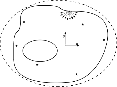
Figure 1: Here we consider the case when $m=2$ and $n=7$. The positions of the agents at a time $t$ are denoted by stars. The solid curves is the set $\{y\in\mathbb{R}^{m}:V(y)=\alpha\}$. The dashed curve is the boundary of $\mathcal{D}^{*}(\infty)$.

Another example where the theorems can be used is when the agents are contained in a geodesic convex and closed subset of a sphere. In this case we can choose $f_{W,m,m}(x_{i},x_{j})$ as the geodesic distance squared between $x_{i}$ and $x_{j}$. If $f_{i}(t,x)$ corresponds to a tangent vector that is inward-pointing [2] relative to the convex hull on the sphere (not to mix up with a convex hull in a Euclidean space) of the positions of the neighbors of agent $i$ at time $t$ (provided it is nonempty otherwise $f_{i}(t,x)=0$), then one can show that Assumption 2.4 is fulfilled.

4.2 Convexity

We continue with a less general case where the decreasing functions are chosen as the Euclidean norm squared of the states and the relative states respectively. Under certain conditions, these choices of functions can be used to show a well known convexity result that, provided the right-hand side of each agent’s dynamics as an element of the tangent space $T_{x_{i}}\mathbb{R}^{m}$ is inward-pointing [2] relative to the convex hull of its neighbors, the system reaches consensus asymptotically [13, 29]. We define the tangent cone to a convex set $S\in\mathbb{R}^{m}$ at the point $y$ as

$$\mathcal{T}(y,S)=\bigg{\{}z\in\mathbb{R}^{m}:\liminf_{\lambda\rightarrow 0}\frac{\text{dist}(y+\lambda z,S)}{\lambda}=0\bigg{\}}.$$

This definition can be found in [13], and $\xi$ is inward-pointing relative to $S$, where $0\neq\xi\in T_{y}\mathbb{R}^{m}$ ($T_{y}\mathbb{R}^{m}$ is the tangent space of $\mathbb{R}^{m}$ at the point $y$), if $\xi$ belongs to the relative interior of $\mathcal{T}(y,S)$. We use the term relative interior, since the dimension of $S$ might be smaller than $m$. Let us denote the convex hull for $\{x_{i}\}_{i=1}^{n}$ by $\text{conv}(\{x_{i}\}_{i=1}^{n})$. Similarly, we can denote the convex hull for the positions of the neighbors of agent $i$ as $\text{conv}(\{x_{j}\}_{j\in\mathcal{N}_{i}})$.

Suppose Assumption 2.4 is fulfilled. We consider the case when

$$V(x_{i})=x_{i}^{T}x_{i}\quad\text{and}\quad W(x_{i},x_{j})=(x_{j}-x_{i})^{T}(x_{j}-x_{i}),$$

where $V$ and $W$ generate the functions $f_{V,m}$ and $f_{W,m,m}$ respectively.

Suppose the functions in $\mathcal{F}$ are Lipschitz in $x$ on $\mathbb{R}^{mn}$, uniformly with respect to $t$, and continuous in $t$. Furthermore, suppose $V$ fulfills Assumption 2.4, then in Theorem 3 we can choose $\widehat{\beta}_{1}(\|x_{i}\|)=\widehat{\beta}_{2}(\|x_{i}\|)=\|x_{i}\|^{2}$, and obtain the result that any closed ball $\bar{B}_{r}$ in $\mathbb{R}^{m}$ is invariant and can be chosen as $\mathcal{D}=\mathcal{D}^{*}(\infty)=\bar{B}_{r}$, and the point $x=0$ is uniformly stable. Thus, by Theorem 3 we obtain the result that if $\mathcal{G}_{\sigma(t)}$ is uniformly strongly connected, then $\mathcal{A}$ is globally quasi-uniformly attractive relative to $\mathcal{D}^{*}(\infty)$. Unless $x_{i}=x_{j}$ for all $j\in\mathcal{N}_{i}$, for any agent $i$ that is furthest away from the origin, $f_{i}(t,x)$ as an element of the tangent space $T_{x_{i}}\mathbb{R}^{m}$ is inward-pointing on the boundary of the closed ball with radius equal to the norm of agent $i$. This is illustrated in Figure 2. An example of this situation is provided in Section 4.5 in the application of reaching consensus for a system of rotation matrices.

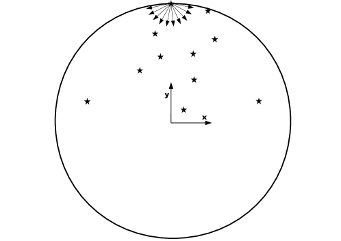
Figure 2: In this case $m=2$. The positions of the agents at a time $t$ are denoted by stars. When at least one of the neighbors of an agent $i$ on the boundary of the ball $\bar{B}_{\max\limits_{k\in\mathcal{V}}\|x_{k}(t)\|,2}$ is located in the interior of the ball, $f_{i}(t,x)\in T_{x_{i}}\mathbb{R}^{2}$ is inward-pointing (relative to the ball).

Suppose not only that $V$ fulfills Assumption 2.4, but also that $W$ fulfills Assumption 2.4. In this case, any closed ball in $\mathbb{R}^{m}$ is invariant and can be chosen as $\mathcal{D}^{*}(\infty)$, but also the largest Euclidean distance between any pair of agents is decreasing. This is illustrated in Figure 3. Now Theorem 3 holds and $\mathcal{A}$ is globally uniformly asymptomatically stable relative to $\mathcal{D}^{*}(\infty)$ if and only if $\mathcal{G}_{\sigma(t)}$ is uniformly quasi-strongly connected. For agent $i$, if $f_{i}(t,x)$ is inward-pointing relative to the convex hull of its neighbors [13, 29], then these conditions are fulfilled.

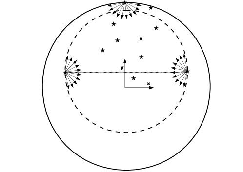
Figure 3: In this case $m=2$. The positions of the agents at some time $t$ are denoted by stars. The solid circle denotes the boundary of the ball with radius $\sqrt{f_{V,m}(x(t))}$ and the dashed circle denotes the boundary of the ball with radius $\sqrt{f_{W,m,m}(x(t))}$. The dashed line denotes the distance between the two agents that are furthest away from each other.

As a special case let

$$f_{i}(t,x)=\sum_{j\in\mathcal{N}_{i}(t)}a_{ij}(t-\gamma_{\sigma}(t))(x_{j}-x_{i}),$$

where $\alpha_{ij}(t)>0$ is continuous, positive and bounded for all $t$. Let us construct the set of functions $\mathcal{F}$ in the following way. There are $2^{n^{2}}$ graphs. For each graph $\mathcal{G}_{k}$ we define a corresponding function

$$\tilde{f}_{k}(x)=\left(\sum_{j\in\mathcal{N}_{1}}\alpha_{ij}(t)(x_{j}-x_{1}),\ldots,\sum_{j\in\mathcal{N}_{n}}\alpha_{ij}(t)(x_{j}-x_{n})\right)^{T}$$

where $\mathcal{N}_{i}$ in this case is the neighborhood of agent $i$ in the graph $\mathcal{G}_{k}$. Now we let

$$\mathcal{F}=\{\tilde{f}_{k}\}_{k=1}^{2^{n^{2}}},$$

and $\sigma\in\mathcal{S}_{|\mathcal{F}|,D,U}$. In the following examples, if $\mathcal{F}$ is not explicitly defined, we assume that $\mathcal{F}$ is the set of functions that has been constructed in the way analogous to this construction, i.e. all the possible right-hand sides.

Now, using the functions

$$V(x_{i})=x_{i}^{T}x_{i}\quad\text{and}\quad W(x_{i},x_{j})=(x_{j}-x_{i})^{T}(x_{j}-x_{i}),$$

with the corresponding functions $f_{V,m}$ and $f_{W,m,m}$ respectively, one can show global uniform asymptotic consensus relative to $\mathcal{D}^{*}(\infty)$.

4.3 Nonlinear scaling

Here we show how the theorems 3 and 3 can be used to assure consensus when the states and the relative states for pairs of agents have been scaled with a nonlinear scale function.

In this context, let us define a nonlinear scale function as follows. The function $g$ is strictly increasing on $[0,\eta)$ where $\eta>0$ and the map

$$h:x_{i}\mapsto\frac{g(\|x_{i}\|)}{\>\>\|x_{i}\|}x_{i}$$

restricted to $B_{\eta,m}$ is a diffeomorphism between $B_{\eta,m}$ and $B_{\eta^{\prime},m}$, where $\eta^{\prime}~{}>~{}0$.

The interesting observation here regards the order of application of $h$. Suppose that

$$f_{i}(t,x)=\sum_{j\in\mathcal{N}_{i}(t)}a_{ij}(t-\gamma_{\sigma}(t))(x_{j}-x_{i}).$$

Within this context, if we define the following map

$${d}(x_{i},x_{j})=x_{j}-x_{i},$$

we can write the function $f_{i}$ as follows

$$f_{i}(t,x)=\sum_{j\in\mathcal{N}_{i}(t)}a_{ij}(t-\gamma_{\sigma}(t)){d}(x_{i},x_{j}),$$

and we know that $f_{i}$, as an element of the tangent space $T_{x_{i}}\mathbb{R}^{m}$, is inward-pointing relative to the convex hull of the neighbors of agent $i$. Consequently, on $B_{\eta,m}$, we can use Theorem 3 together with Theorem 3 in order to show consensus when the graph $\mathcal{G}(t)$ is uniformly quasi-strongly connected. Now, for each pair of agents, if we modify $f_{i}$ into the following form

$$f_{i}^{\prime}(t,x)=\sum_{j\in\mathcal{N}_{i}(t)}a_{ij}(t-\gamma_{\sigma}(t))h({d}(x_{i},x_{j})),$$

this new function still fulfills the same convexity assumption. However, if we reverse the order of application of the functions $h$ and ${d}$ we get the following modified version of $f_{i}$

$$f_{i}^{\prime\prime}(t,x)=\sum_{j\in\mathcal{N}_{i}(t)}a_{ij}(t-\gamma_{\sigma}(t)){d}(h(x_{i}),h(x_{j})),$$

and in this case it is not necessarily true that $f_{i}^{\prime\prime}(t,x)$ as an element of $T_{x_{i}}\mathbb{R}^{m}$ is inward-pointing relative to the convex hull of the neighbors of agent $i$. However, consensus can be guaranteed on $B_{\eta,m}$ by Theorem 3 when the graph $\mathcal{G}(t)$ is uniformly strongly connected by using the function $V(x_{i})=x_{i}^{T}x_{i}$ in Theorem 3.

4.4 Avoiding discontinuities

Suppose that $\mathcal{F}$ contains only time-invariant functions, $\sigma\in\mathcal{S}_{|\mathcal{F}|,D,U}$ and Assumption 2.4 holds. We show how it is possible to modify the system defined by $\mathcal{F}$ and $\sigma$ into a system where the right-hand side is no longer discontinuous in $t$. Close to each switching time we can modify the system so that there is a continuous in time transition between the two time-invariant functions that are being switched between. For the modified system where there are no longer any discontinuities in $t$, Assumption 2.4 still holds and if there is a $V$ such that Assumption 2.4 holds for this $V$ for the discontinuous system (or a $W$ such that Assumption 2.4 holds for this $W$ for the discontinuous system), then Assumption 2.4 holds for $V$ (or Assumption 2.4 holds for $W$) for the modified continuous system.

We start by extending $\mathcal{F}$ with time varying functions to a finite set of functions $\mathcal{F}^{\prime}$ (Lipschitz in $x$ on $\mathcal{D}$, uniformly with respect to $t$), where $\mathcal{F}^{\prime}$ contains functions that serve as continuous in time transitions between functions in $\mathcal{F}$. For $\sigma\in\mathcal{S}_{|\mathcal{F}^{\prime}|,D,U}$ we create a $\sigma^{\prime}\in\mathcal{S}_{|\mathcal{F}^{\prime}|,D,U}$ in the following way. Let $\tau_{D}^{\sigma^{\prime}}<\tau_{D}^{\sigma}$. At each switching time $\tau_{k}$ of $\sigma$, we squeeze in an extra interval of length $\tau_{D}^{\sigma^{\prime}}$ during which the neighbor set $\mathcal{N}^{\sigma^{\prime}}_{i}$ of each agent $i$ is equal to $\mathcal{N}^{\sigma}_{i}(\tau_{k-1})\cup\mathcal{N}^{\sigma}_{i}(\tau_{k})$. These added time intervals can be seen as transition periods, during which there is a continuous in time transition between two functions in $\mathcal{F}$.

We extend $\mathcal{F}$ to $\mathcal{F}^{\prime}$ in the following way. First we define a continuous function

$$\alpha:(-\infty,\infty)\rightarrow[0,1],$$

such that $\alpha(0)=1$ and $\alpha(\tau_{D}^{\sigma^{\prime}})=0$. Secondly, for each pair of functions $(\tilde{f}_{i},\tilde{f}_{j})$ where $\tilde{f}_{i}$ and $\tilde{f}_{j}$ belong to $\mathcal{F}$, we define a function

$$\tilde{f}_{(i,j)}(t,x)=\alpha(t)\tilde{f}_{i}(x)+(1-\alpha(t))\tilde{f}_{j}(x).$$

The set of functions $\mathcal{F}^{\prime}$ is the set of all functions $\tilde{f}_{i}$ and $\tilde{f}_{(i,j)}$. At each switching time of the original system, between the right-hand side $\tilde{f}_{i}$ and $\tilde{f}_{j}$, we now squeeze in the function $\tilde{f}_{(i,j)}$ during a time period of length $\tau_{D}^{\sigma^{\prime}}$ in the new system. Note that we can make $\tau_{D}^{\sigma^{\prime}}$ much smaller than $\tau_{D}^{\sigma}$.

If all functions in $\mathcal{F}$ are time-invariant $\mathcal{C}^{1}$ functions in $x$, and we want the new continuous right-hand side to be $\mathcal{C}^{1}$ in $t$ when $x$ is regarded as a function of $t$, we impose the additional requirement that $\dot{\alpha}(0)=0$ and $\dot{\alpha}(\tau_{D}^{\sigma^{\prime}})=0$. A function fulfilling these requirements is

$$\alpha(t)=\frac{1}{2}+\frac{1}{2}\cos\left(\frac{t\pi}{\tau_{D}^{\sigma^{\prime}}}\right).$$

We now proceed with some other application oriented examples.

4.5 Consensus on $SO(3)$ using the Axis-Angle Representation

Here we have a system of $n$ rotation matrices in $SO(3)$ (controlled on a kinematic level) shall asymptotically reach consensus in the rotation matrices. For a rotation matrix $R_{i}$ there is a corresponding vector $x_{i}$, referred to as the Axis-Angle Representation of $R_{i}$. Locally around the identity matrix, in terms of kinematics we have that

$$\dot{R}_{i}=R_{i}\widehat{\omega}_{i}\quad\quad\text{or}\quad\quad\dot{x}_{i}={L}_{x_{i}}\omega_{i},$$

where

$${L}_{{x}_{i}}=I_{3}+\frac{\widehat{{x}}_{i}}{2}+\frac{1}{\|{x}_{i}\|^{2}}\bigg{(}1-\frac{\text{sinc}(\|{x}_{i}\|)}{\text{sinc}^{2}(\frac{\|{x}_{i}\|}{2})}\bigg{)}\widehat{x}_{i}^{2},$$

and $\widehat{\omega}_{i}$, $\widehat{x}_{i}$ are the skew-symmetric matrices generated by $\omega_{i},x_{i}\in\mathbb{R}^{3}$ respectively, and we require that $x_{i}(t_{0})\in B_{\pi,3}$ for all $i$. Now we consider the case when

$$\omega_{i}=\sum_{j\in\mathcal{N}_{i}(t)}\alpha_{ij}(t-\gamma_{\sigma}(t))(x_{j}-x_{i}),$$

where the continuous function $\alpha_{ij}(t)$ is positive and bounded, and $\sigma\in\mathcal{S}_{|\mathcal{F}|,D,U}$. The symmetric part of the matrix ${L}_{x_{i}}$ is positive definite on $B_{\pi,3}$, and the system is at an equilibrium if and only if $x=(x_{1},\ldots,x_{n})^{T}\in\mathcal{A}$.

Let $V(x_{i})=x_{i}^{T}x_{i}$. By observing that $x_{i}^{T}{L}_{x_{i}}=x_{i}^{T}$, it is easy to show that Assumption 2.4 holds for $V$. We can apply Theorem 3 with $\widehat{\beta}_{1}(\|x_{i}\|)=\widehat{\beta}_{2}(\|x_{i}\|)=\|x_{i}\|^{2}$, and show that any ball $\bar{B}_{r,3}$ is invariant for $r<\pi$ and may serve as $\mathcal{D}=\mathcal{D}^{*}(\infty)$. Also, by Theorem 3, if the graph $\mathcal{G}_{\sigma(t)}$ is uniformly strongly connected, then $\mathcal{A}$ is globally quasi-uniformly attractive.

4.6 Consensus on $SO(3)$ for networks of cameras using the epipoles

This example is based on the work in [18, montijano2011multi], where a more detailed description can be obtained. Undefined terminology that is used in this example can be found in any standard text book on computer vision such as [15]. This example also regards consensus for rotation matrices, but the setting is a bit different and the rotations are restricted to be only around one common axis. We consider a system of $n$ robots positioned in the two-dimensional plane. Each robot is equipped with a camera and is at each time observing a subset of the other robots. Since the rotational axes are fixed and equal, we only need the scalar $\theta_{i}$ in order to represent the rotation of each agent $i$, where $\theta_{i}$ is the angle of rotation. In the context of this example, instead of letting $\theta_{i}\in[0,\pi)$, we let $\theta_{i}\in(-\pi,\pi)$. We assume that all the cameras have the same intrinsic parameters.

The robots are not moving and are only rotating. The position of each robot $i$ in the world coordinate frame is given by $x_{i}\in\mathbb{R}^{2}$. The position of agent $j$ in the body frame of agent $i$ is given by

$$x_{ij}(\theta_{i})=R(\theta_{i})(x_{j}-x_{i}),$$

where

$$R(\theta_{i})=\begin{bmatrix}\cos(\theta_{i})&-\sin(\theta_{i})\\ \sin(\theta_{i})&\cos(\theta_{i})\end{bmatrix}.$$

Let

$$\psi_{ij}(\theta_{i})=\text{arctan}\left(\frac{x_{ijx}}{x_{ijy}}\right),$$

where $x_{ijx}$ and $x_{ijy}$ are the two components of $x_{ij}$.

Now, instead of measuring the rotation directly, using stereo vision one retrieves the epipoles as certain nullspace vectors of the so called fundamental matrix. The fundamental matrix defines the (epipolar) geometric relationship between two images [15], and should not be mixed up with the fundamental matrix in the solution of a linear time-invariant dynamical system. We will only consider the $x$-component (the first component) of these two-dimensional epipole vectors, which are defined as

$$e_{ij}=\alpha\tan(\psi_{ij}),\quad e_{ji}=\alpha\tan(\psi_{ij}-\theta_{ij}),$$

where $\theta_{ij}=\theta_{j}-\theta_{i}$ and $\alpha=1$ if the cameras are calibrated, i.e., the focal length is known (we assume that the position of the principal point is known in the image plane), otherwise $\alpha>0$ is unknown.

Let us define

$$\omega_{ij}=\arctan\left(\frac{e_{ij}}{\beta}\right)-\arctan\left(\frac{e_{ji}}{\beta}\right)$$

where $\beta>0$ is a constant to choose.

We define $\theta(t)=(\theta_{1}(t),\ldots,\theta_{n}(t))^{T}$ and the region

$$\mathcal{D}=\{\theta:-\theta_{M}\leq\theta_{i}\leq\theta_{M}\text{ for }i=1,\ldots,n\},$$

where $0<\theta_{M}\ll\pi/2$. The set $\mathcal{D}$ could be seen as being a function of $\theta_{M}$. Furthermore, we assume ${x_{ijx}(0)}/{x_{ijy}(0)}=1$ for all $i,j$, in which case the robots or the cameras are standing on a line and are oriented in the same direction that forms an angle of $\pi/4$ to the direction of the line. This means that $\psi_{ij}\in\{-\pi/4,3\pi/4\}$ for all $i,j$.

Let us choose the dynamics for the system as

$$\dot{\theta}_{1}= \sum_{j\in\mathcal{N}_{1}(t)}\alpha_{1j}(t-\gamma_{\sigma}(t))\omega_{1j},$$

$$\vdots$$

$$\dot{\theta}_{n}= \sum_{j\in\mathcal{N}_{n}(t)}\alpha_{nj}(t-\gamma_{\sigma}(t))\omega_{nj}.$$

We assume that $\alpha_{ij}(t)$ is continuous, positive and bounded, and $\sigma\in\mathcal{S}_{|\mathcal{F}|,D,U}$. Provided $\theta_{M}$ is sufficiently small, on $\mathcal{D}$ it can be shown that $\omega_{ij}$ is Lipschitz for all $(i,j)\in\mathcal{V}\times\mathcal{V}$. It is obvious that Assumption 2.4 holds. We choose $\theta_{M}$ small enough so that $|\omega_{ij}|<\pi/2$ on $\mathcal{D}$. According to [18], it is true that

$$\theta_{ij}(t)\neq 0\Longrightarrow\theta_{ij}(t)\omega_{ij}(t)>0.$$ (2)

Let us now consider the function $V(\theta_{i})=\theta_{i}^{2}$, where

$$\frac{d}{dt}{V}(\theta_{i})=2\theta_{i}\sum_{j\in\mathcal{N}_{i}(t)}\alpha_{ij}(t)\omega_{ij}.$$

Suppose $i\in\mathcal{I}_{V}(t,t)$, and $\theta_{j}(t)=\theta_{i}(t)$ for all $j\in\mathcal{N}_{i}(t)$, then it follows that $\dot{V}(\theta_{i}(t))=0$. Now, consider the situation where $i\in\mathcal{I}_{V}(t,t)$ and there is at least one $j$ such that $\theta_{j}(t)\neq\theta_{i}(t)$ when $j\in\mathcal{N}_{i}(t)$. Since $i\in\mathcal{I}_{V}(t,t)$, if $\theta_{i}\neq\theta_{j}$, using (2) we get that

$$\theta_{i}\omega_{ij}<0.$$

Hence, Assumption 2.4 also holds.

In Theorem 3 we can now choose $\widehat{\beta}_{1}(|\theta_{i}|)=\widehat{\beta}_{2}(|\theta_{i}|)=|\theta_{i}|^{2}$ and reach the conclusion that $\mathcal{D}$ is positively invariant and $\mathcal{D}^{*}(\infty)=\mathcal{D}$. The point $0$ is uniformly stable. Furthermore, according to Theorem 3, $\mathcal{A}$ is globally quasi-uniformly attractive relative to $\mathcal{D}^{*}(\infty)$ if $\mathcal{G}_{\sigma(t)}$ is uniformly strongly connected. But we can actually weaken the assumptions on the graph $\mathcal{G}_{\sigma(t)}$.

Let us consider the function $W(\theta_{i},\theta_{j})=(\theta_{j}-\theta_{i})^{2}$, where

$$\frac{d}{dt}{W}(\theta_{i},\theta_{j})$$

$$=2(\theta_{j}-\theta_{i})\left(\sum_{k\in\mathcal{N}_{j}(t)}\alpha_{jk}(t-\gamma_{\sigma}(t))\omega_{jk}-\sum_{l\in\mathcal{N}_{l}(t)}\alpha_{il}(t-\gamma_{\sigma}(t))\omega_{il}\right).$$

If $(i,j)\in\mathcal{J}_{V}(t,t)$, we can without loss of generality assume that $\theta_{j}\geq\theta_{k}$ and that $\theta_{i}\leq\theta_{k}$ for all $k\in\mathcal{V}$. This implies that $\text{sign}(\theta_{ij})=\text{sign}(\theta_{kj})=\text{sign}(\theta_{il})=1$ for all $k,l\in\mathcal{V}$, so from (2) we get that $\text{sign}(\theta_{ij})\text{sign}(\omega_{jk})=-1$ and $\text{sign}(\theta_{ij})\text{sign}(\omega_{il})=1$. Thus Assumption 2.4 holds for $f_{W,m,m}$ and Theorem 3 can be used. Thus, when $x(t)\in\mathcal{D}^{*}(\infty)$ it follows that $\mathcal{A}$ is globally uniformly asymptotically stable relative to $\mathcal{D}^{*}(\infty)$ if and only if $\mathcal{G}_{\sigma(t)}$ is uniformly quasi-strongly connected.

4.7 Stabilization

Let us now, as a special case of the consensus problem, consider the stabilization problem, where we use our consensus results in order to provide known conditions for when $\{0\}$ is asymptotically stable for a system

$$\dot{y}=g(t,y),$$ (3)

where $y\in\mathbb{R}^{m}$.

We show that this problem is a special case of a consensus problem with two agents in $\mathbb{R}^{m}$, so that we can use Theorem 3 in order to show that $\{0\}$ is globally uniformly asymptotically stable relative to some compact invariant set in $\mathbb{R}^{m}$.

Proposition .

Suppose there is an invariant compact set $\mathcal{D}^{\prime}\subset\mathbb{R}^{m}$ containing the point $0$ and a finite set $\mathcal{F}^{\prime}=\{\tilde{f}_{1}^{\prime},\ldots,\tilde{f}_{|\mathcal{F}^{\prime}|}^{\prime}\}$ of functions that are piecewise continuous in $t$ and Lipschitz in $y$ on $\mathcal{D}^{\prime}$, uniformly with respect to $t$. For each function $\tilde{f}_{k}^{\prime}$ it holds that $\tilde{f}_{k}^{\prime}(t,0)=0$ for all $k$ and all $t$. Furthermore, $\sigma\in\mathcal{S}_{|\mathcal{F}^{\prime}|,D,U}$ and the right-hand side of (3) is

$$g(t,y)=\tilde{f}_{\sigma(t)}^{\prime}(t-\gamma_{\sigma}(t),y).$$

If there is a positive definite function $V(y)$, which is continuously differentiable on an open set containing $\mathcal{D}^{\prime}$ such that

$$\nabla V(y)\tilde{f}_{i}^{\prime}(t,y)<0$$

for all $i\in\{1,\ldots,|\mathcal{F}^{\prime}|\}$, all $t$ and nonzero $y$ in $\mathcal{D}^{\prime}$, then $\{0\}$ is globally uniformly asymptotically stable relative to $\mathcal{D}^{\prime}$.

 Proof: The set $\mathcal{D}^{\prime}$ is assumed to be invariant for any choices of switching signal functions in $\mathcal{S}_{|\mathcal{F}^{\prime}|,D}$. Let us define a system of two agents, agent 1 and agent 2. Based on the set $\mathcal{F}^{\prime}$ we create a new set $\mathcal{F}^{\prime\prime}$ of functions with range $\mathbb{R}^{2m}$ in the following way

$$\mathcal{F}^{\prime\prime}=\{(\tilde{f}^{\prime}_{1}(t,y_{2}-y_{1}),0)^{T},\ldots,(\tilde{f}^{\prime}_{|\mathcal{F}^{\prime}|}(t,y_{2}-y_{1}),0)^{T}\}.$$

Now, for all $t\geq 0$ and for all $\sigma\in\mathcal{S}_{|\mathcal{F}^{\prime\prime}|,D}$ we define

$$\mathcal{N}_{1}^{\sigma}(t)=\{1,2\}\quad\text{ and }\quad\mathcal{N}_{2}^{\sigma}(t)=\{2\}.$$

The system dynamics for this extended system is given as

$$\dot{y}_{1} =\tilde{f}^{\prime}_{1}(t-\gamma_{\sigma}(t),y_{2}-y_{1}),$$

$$\dot{y}_{2} =0.$$

This system fulfills Assumption 2.4 and we define a function $W$ as

$$W(y_{1},y_{2})=V(y_{2}-y_{1}).$$

The function $W$ fulfills Assumption 2.4. Now, if the initial positions of $y_{1}(t)$ and $y_{2}(t)$ are $y_{1}^{0}\in\mathcal{D}^{\prime}$ and $y_{2}^{0}=0\in\mathcal{D}^{\prime}$ respectively, we see that the dynamics for the extended system is equivalent to the original system (1). For the extended system, the set $\mathcal{D}^{\prime}\times\{0\}\subset((\mathcal{D}^{\prime})^{2})^{*}(\infty)$. Since $\mathcal{G}_{\sigma(t)}$ is uniformly quasi-strongly connected, $\mathcal{A}$ is globally uniformly asymptotically stable relative to $((\mathcal{D}^{\prime})^{2})^{*}(\infty)$. Since $y_{2}(t)=0$ for all $t$, we see that the state will converge to the point $(0,0)^{T}\in\mathbb{R}^{2m}$ in the extended system. $\blacksquare$

5 Proofs

In this section we provide the proofs. Theorem 3 is proven directly, whereas for the two other theorems, in order to make the proofs more comprehensible, we first introduce some lemmas, used as building blocks for the final proof.

Proof of Lemma 2.1: We can construct the $\sigma^{\prime}$ as follows. Let us first choose $\tau_{D}^{\sigma^{\prime}}=\tau_{D}^{\sigma}$ and $\tau_{U}^{\sigma^{\prime}}\geq 2\tau_{D}^{\sigma}$. For any $k$ such that $\tau_{k+1}-\tau_{k}>\tau_{U}^{\sigma^{\prime}}$, we split $[\tau_{k},\tau_{k+1})$ into a partition of smaller half-open intervals each with equal length smaller than $\tau_{U}^{\sigma^{\prime}}$ but larger than $\tau_{D}^{\sigma^{\prime}}$. On these half-open intervals $\sigma^{\prime}(t)=\sigma(t)$. For all $k$ such that $\tau_{k+1}-\tau_{k}\leq\tau_{U}^{\sigma^{\prime}}$ we let $\sigma^{\prime}(t)=\sigma(t)$ for $t\in[\tau_{k},\tau_{k+1})$. $\blacksquare$

Proof of Lemma 2.1: Let $\tau_{U}=\tau_{U}^{\sigma}$ and $\tau_{D}=\tau_{D}^{\sigma}$. The function $\sigma^{\prime}$ is constructed in a way similar to the procedure in the proof of Lemma 2.1, but here the number of half-open intervals that $[\tau_{k},\tau_{k+1})$ is split into is bounded from above by $\lfloor\tau_{U}/\tau_{D}\rfloor$.

We define the partition of intervals as follows

$$[\tau_{k},\tau_{k+1})= \left(\bigcup_{i=1}^{\lfloor(\tau_{k+1}-\tau_{k})/\tau_{D}\rfloor-1}[\tau_{k}+(i-1)\tau_{D},\tau_{k}+i\tau_{D})\right)$$

$$\>\>\>\quad\cup[\tau_{k}+(\lfloor(\tau_{k+1}-\tau_{k})/\tau_{D}\rfloor-1)\tau_{D},\tau_{k+1}).$$

We define $\mathcal{F}^{\prime}$ as follows

$$\mathcal{F}^{\prime}=\{ \tilde{f}_{1}^{\prime}=\tilde{f}_{1}(t,x),$$

$$\tilde{f}_{2}^{\prime}=\tilde{f}_{1}(t+\tau_{D},x),\ldots,$$

$$\tilde{f}_{\lfloor\tau_{U}/\tau_{D}\rfloor}^{\prime}=\tilde{f}_{1}(t+(\lfloor\tau_{U}/\tau_{D}\rfloor-1)\tau_{D},x),\ldots,$$

$$\tilde{f}_{\lfloor\tau_{U}/\tau_{D}\rfloor(N-1)+1}^{\prime}=\tilde{f}_{N}(t+\tau_{D},x),\ldots,$$

$$\tilde{f}_{\lfloor\tau_{U}/\tau_{D}\rfloor N}^{\prime}=\tilde{f}_{N}(t+(\lfloor\tau_{U}/\tau_{D}\rfloor-1)\tau_{D},x)\},$$

where $N=|\mathcal{F}|$. The set $\mathcal{F}^{\prime}$ is constructed by creating $\lfloor\tau_{U}/\tau_{D}\rfloor-1$ number of new time-shifted functions from each function $\tilde{f}_{i}\in\mathcal{F}$.

Now $\sigma^{\prime}$ is constructed by choosing a function in $\mathcal{F}^{\prime}$ on each half-open interval in each partition so that

$$\tilde{f}_{\sigma(t)}(t,x)=\tilde{f}_{\sigma^{\prime}(t)}^{\prime}(t,x)$$

for all $t$ and $x\in\mathcal{D}$. $\blacksquare$

Proof of Lemma 2.3: We only prove the first statement for $f_{{V},m}$, the procedure in order to prove the second statement for $f_{{V},m,m}$ is similar and hence omitted.

Since $V$ is Lipschitz in $x$ on $\mathcal{D}$ it follows that $f_{V,m}$ is Lipschitz in $x$ on $\mathcal{D}$. Since $f_{V,m}$ is Lipschitz in $x$, it follows that

$$D^{+}(f_{V,m}(x(t)))=D^{+}_{f_{V,m}}(f_{V,m}(x^{*})),$$

where

$$D^{+}_{f_{V,m}}(f_{V,m}(x^{*}))=\lim_{\epsilon\downarrow 0}\sup\frac{f_{f_{V,m}}(t+\epsilon,x_{0}+\epsilon f_{V,m}(t,x^{*}))}{\epsilon}$$

and $x^{*}=x(t)$. This result can be obtained from Chapter 1 in [33]. In [28] it is formulated as a Theorem (Theorem 4.1 in Appendix I).

The next step is to prove that

$$D^{+}_{f_{V,m}}(f_{V,m}(t,x^{*}))=\max_{i\in\mathcal{I}_{V}(t,t)}\frac{d}{dt}{V}(x_{i}(t)).$$

This result can for example be obtained from Theorem 2.1. in [6]. $\blacksquare$

Proof of Lemma 2.4: Since $\mathcal{D}$ is compact, we only need to verify that $\mathcal{D}^{*}(\tilde{t})$ is closed in order to show that $\mathcal{D}^{*}(\tilde{t})$ is compact. Suppose there is $x_{0}\notin\mathcal{D}^{*}(\tilde{t})$, such that there is a sequence $\{x_{0}^{i}\}_{i=1}^{\infty}$ that converges to $x_{0}$, where each element in the sequence is in $\mathcal{D}^{*}(\tilde{t})$. We would like to obtain a contradiction by showing that the solution $x^{\sigma}(t,t_{0},x_{0})$ does exist in $\mathcal{D}$ on the interval $[t_{0},t_{0}+\tilde{t})$ for any $t_{0}$, and $\sigma\in\mathcal{S}_{|\mathcal{F}|,D}$.

By using the fact that $\mathcal{D}$ is compact and that the right-right side of (1) is uniformly Lipschitz in $x$ on $\mathcal{D}$ and piecewise continuous in $t$, we can use the Continuous Dependency Theorem of initial conditions in order to guarantee that $\{x^{\sigma}(t,t_{0},x_{0}^{i})\}_{i=1}^{\infty}$ is a Cauchy sequence for arbitrary $t\in[t_{0},t_{0}+\tilde{t})$. Now we know, since $\mathcal{D}$ is compact, that

$$x^{*}(t)=\lim_{i\rightarrow\infty}x^{\sigma}(t,t_{0},x_{0}^{i})$$

exists and $x^{*}(t)\in\mathcal{D}$. We want to prove that $x^{*}(t)$ is the solution for (1) on $[t_{0},t_{0}+\tilde{t})$ for the given $\sigma$, $t_{0}$ and $x_{0}$.

$$x^{*}(t) =\lim_{i\rightarrow\infty}x^{\sigma}(t,t_{0},x_{0}^{i})$$

$$=\lim_{i\rightarrow\infty}\int_{t_{0}}^{t}f(s,x^{\sigma}(s,t_{0},x_{0}^{i}))ds$$

$$=\int_{t_{0}}^{t}\lim_{i\rightarrow\infty}f(s,x^{\sigma}(s,t_{0},x_{0}^{i}))ds$$

$$=\int_{t_{0}}^{t}f(s,x^{*}(s)).$$

Hence, $x^{*}(t)$ is contained $\mathcal{D}$ for all $t$, but since $\sigma$ and $t_{0}$ were arbitrary, it follows that $x_{0}\in\mathcal{D}^{*}(\tilde{t})$ which is a contradiction.

Now we prove the statement that $\mathcal{D}^{*}(\infty)$ is invariant. Suppose $x_{0}\in\mathcal{D}^{*}(\infty)$ is arbitrary and let

$$y=x^{\sigma_{1}}(t_{1},t_{0},x_{0})$$

for $\sigma_{1}\in\mathcal{S}_{|\mathcal{F}|,D}$ and $t_{1}\geq t_{0}$. Consider $x^{\sigma_{2}}(t,t_{1}^{\prime},y)$ for some arbitrary $\sigma_{2}\in\mathcal{S}_{|\mathcal{F}|,D}$ and $t_{1}^{\prime}$. We need to show that $x^{\sigma_{2}}(t,t_{1}^{\prime},y)$ is contained in $\mathcal{D}$ for all $t\geq t_{1}^{\prime}$.

We define

$$\sigma(t)=\begin{cases}\sigma_{1}(t-(t_{1}^{\prime}-t_{1}))&\text{if }t<t_{1}^{\prime},\\ \sigma_{2}(t)&\text{if }t\geq t_{1}^{\prime}.\end{cases}$$

which is contained in $\mathcal{S}_{|\mathcal{F}|,D}$. Thus

$$x^{\sigma_{2}}(t,t_{1}^{\prime},y)=x^{\sigma}(t,t_{0}+(t_{1}^{\prime}-t_{1}),x_{0})$$

which is contained in $\mathcal{D}$ for all $t\geq t_{0}$ since $x_{0}\in\mathcal{D}^{*}(\infty)$. Thus $y\in\mathcal{D}^{*}(\infty)$. $\blacksquare$

Proof of Theorem 3: Since the origin is an interior point of $\mathcal{D}$, there is a ball ${B}_{\epsilon,m}$ such that $({B}_{\epsilon,m})^{n}\subset\mathcal{D}$ and $\epsilon>0$. Suppose $x_{0}\in({B}_{\epsilon,m})^{n}$, then there is a closed ball

$$\bar{B}_{\epsilon^{\prime},mn}(x_{0})\subset({B}_{\epsilon,m})^{n}$$

with $\epsilon^{\prime}>0$. Now according to Theorem 3.1. in [12], there is a $\delta^{\prime}>0$ such that the system has a unique solution ${x}(t,t_{0},x_{0})$ on $[t_{0},t_{0}+\delta^{\prime}]$. We choose $[t_{0},t_{0}+{T^{\prime}})$ as the maximal half-open interval of existence of the unique solution. We know there are class $\mathcal{K}$ functions $\beta_{1}$ and $\beta_{2}$ such that

$$\beta_{1}(\|y\|)\leq V(y)\leq\beta_{2}(\|y\|)$$

for $y\in\mathbb{R}^{m}$.

Now, using property (2) of Assumption 2.4 we get from the Comparison Lemma (Lemma 3.4 in [12]), that

$$f_{V,m}({x}(t))\leq f_{V,m}({x}_{0})$$

for $t\in[t_{0},t_{0}+{T}^{\prime}).$ Now let $\delta=\beta_{2}^{-1}(\beta_{1}(\epsilon))$. We suppose that $x_{0}$ was chosen such that

$$x_{i}(t_{0})\in\bar{B}_{\delta,m}\subset\bar{B}_{\epsilon,m}\text{ for all }i.$$

It follows that for $t\in[t_{0},t_{0}+T^{\prime})$,

$$\max_{i\in\{1,\ldots,n\}}\|x_{i}(t)\|=\beta_{1}^{-1}(\beta_{1}(\max_{i\in\{1,\ldots,n\}}\|x_{i}(t)\|))$$

$$=\beta_{1}^{-1}(\max_{i\in\{1,\ldots,n\}}\beta_{1}(\|x_{i}(t)\|))\leq\beta_{1}^{-1}(f_{V,m}(x(t)))$$

$$\leq\beta_{1}^{-1}(f_{V,m}(x(t_{0})))\leq\beta_{1}^{-1}(\max_{i\in\{1,\ldots,n\}}\beta_{2}(\|x_{i}(t_{0})\|))$$

$$\leq\beta_{1}^{-1}(\beta_{2}(\max_{i\in\{1,\ldots,n\}}(\|x_{i}(t_{0})\|)))\leq\beta_{1}^{-1}(\beta_{2}(\delta))=\epsilon.$$

Now it follows by using Theorem 3.3 in [12], that the solution will stay in $(\bar{B}_{\epsilon,m})^{n}$ for arbitrary times larger than $t_{0}$, i.e., $T^{\prime}=\infty$. $\blacksquare$

In the following lemma we use the positive limit set $L^{+}(x_{0},t_{0})$ of the solution
$x(t,t_{0},x_{0})$ when $x_{0}\in\mathcal{D}^{*}(\infty)$ (we assume that $\sigma\in\mathcal{S}_{|\mathcal{F}|,D}$ is fixed here). This limit set exists and is compact, and $x(t)$ approaches it as the time goes to infinity, however it is not guaranteed to be invariant which is the case for an autonomous system. Now, in the case that $x_{0}\in\mathcal{D}^{*}(\infty)$, the set $L^{+}(x_{0},t_{0})$ is contained in $\mathcal{D}^{*}(\infty)$, so any alternative solution of (1) that starts in $L^{+}(x_{0},t_{0})$ will remain in $\mathcal{D}^{*}(\infty)$.

Lemma .

Suppose that $x_{0}\in\mathcal{A}^{c}\cap\mathcal{D}^{*}(\infty)$ and that Assumption 2.4 (2) holds. Suppose that there is a non-negative function $\beta(y,\tilde{t})$ that is increasing in $\tilde{t}$ for $y\in\mathcal{A}^{c}\cap\mathcal{D}^{*}(\infty)$. Furthermore, suppose that for $y\in\mathcal{A}^{c}\cap\mathcal{D}^{*}(\infty)$, there is $\tilde{t}^{\prime}(y)>0$ such that for $\tilde{t}\geq\tilde{t}^{\prime}(y)$ it holds that $\beta(y,\tilde{t})>0$.

If

$$f_{V,m}(x(t_{0}+\tilde{t},t_{0},x_{0}))-f_{V,m}(x_{0})\leq-\beta(x_{0},\tilde{t}),$$

then $x(t)\rightarrow\mathcal{A}$ as $t\rightarrow\infty$ for all $t_{0}$.

Furthermore, if $\beta$ is lower semi-continuous in $y$, and $\tilde{t}^{\prime}$ is independent of $y$, then $\mathcal{A}$ is globally quasi-uniformly attractive relative to $\mathcal{D}^{*}(\infty)$.

Proof: Let us consider an arbitrary $x_{0}\in\mathcal{A}^{c}\cap\mathcal{D}^{*}(\infty)$ and $t_{0}$ for which the solution $x(t,t_{0},x_{0})$ generates the limit set $L^{+}(x_{0},t_{0})\subset\mathcal{D}^{*}(\infty)$. From the fact that $f_{V,m}(x(t))$ is continuous in $t$, the fact that $f_{V,m}(x(t))$ is decreasing and the fact that $x(t)$ is contained in the compact set $\mathcal{D}^{*}(\infty)$, it follows that $f_{V,m}(x(t,t_{0},x_{0}))$ converges to a lower bound $\alpha(x_{0},t_{0})\geq 0$ as $t\rightarrow\infty$. Suppose $L^{+}(x_{0},t_{0})\not\subset\mathcal{A}$. We want to prove the lemma by showing that this assumption leads to a contradiction. Let $t_{1}\geq t_{0}$ be arbitrary and $y_{1}$ be an arbitrary point in $L^{+}(x_{0},t_{0})\cap\mathcal{A}^{c}$. Since $y_{1}\in\mathcal{D}^{*}(\infty)$, we know that $x(t,t_{1},y_{1})$ exists and is contained in $\mathcal{D}^{*}(\infty)$ for any time $t>t_{1}$.

Since each function in $\mathcal{F}$ is uniformly Lipschitz continuous in $x$ with respect to $t$ on the compact set $\mathcal{D}^{*}(\infty)$ and the number of functions in $\mathcal{F}$ is finite, we can use the Continuous Dependency Theorem of initial conditions (e.g., Theorem 3.4 in [12]). For $\epsilon>0$ and $\tilde{t}\geq 0$ there is $\delta(\epsilon,\tilde{t})>0$ such that

$$\|y_{1}-y_{1}^{\prime}\|\leq\delta\Longrightarrow\|f_{V,m}(x(t_{2},t_{1},y_{1}))-f_{V,m}(x(t_{2},t_{1},y_{1}^{\prime}))\|\leq\epsilon,$$

where $t_{2}=t_{1}+\tilde{t}$. Let us now choose $\tilde{t}\geq\tilde{t}^{\prime}(y_{1})$ and $\epsilon=\beta(y_{1},\tilde{t})/2,$ from which it follows that $\epsilon$ is guaranteed to be positive. Since $y_{1}\in L^{+}(x_{0},t_{0})$, there is $t^{\prime}>t_{0}$ such that $\|y_{1}-x(t^{\prime},t_{0},x_{0})\|\leq\delta$. We choose $t_{1}=t^{\prime}$ and $y_{1}^{\prime}=x(t^{\prime},t_{0},x_{0})$. But then since $f_{V,m}(x(t_{2},t_{1},y_{1}))\leq\alpha-\beta(y_{1},\tilde{t})$ it follows that $f_{V,m}(x(t_{2},t_{0},x_{0}))\leq\alpha-\beta(y_{1},\tilde{t})/2=\alpha-\epsilon$. Since $\epsilon>0$, this contradicts the fact that $\alpha$ is a lower bound for $f_{V,m}$.

Now we shall prove the second part of the statement. We prove this by a contradiction argument. Suppose there is $\eta>0$ such that there is no $T(\eta)\in\mathbb{R}^{+}$ such that

$$\min_{t\in[t_{0},t_{0}+T(\eta)]}\text{dist}(x(t,t_{0},x_{0}),\mathcal{A})<\eta$$

for all $x_{0}\in\mathcal{D}^{*}(\infty)$ and all $t_{0}$. Let

$$\beta_{\min}=\min_{z\in\mathcal{D}^{*}(\infty)\cap\{y:\text{dist}(y,\mathcal{A})\geq\eta\}}\beta(z,\tilde{t}^{\prime})>0.$$

Now, for each positive integer $N$ there is $t_{0}(N)\geq 0$ and $x_{0}(N)\in\mathcal{D}^{*}(\infty)$ such that

$$\min_{t\in[t_{0}(N),t_{0}(N)+N\tilde{t}^{\prime}]}\text{dist}(x(t,t_{0}(N),x_{0}(N)),\mathcal{A})\geq\eta,$$

otherwise we can choose $T(\eta)=N\tilde{t}$, but we assumed that there is no such $T(\eta)$. We have that

$$f_{V,m}(x(t,t_{0}(N)+N\tilde{t}^{\prime},x_{0}(N)))-f_{V,m}(x(t,t_{0}(N),x_{0}(N)))\leq-N\beta_{\min}.$$

Now,

$$f_{V,m}(x(t,t_{0}(N)+N\tilde{t}^{\prime},x_{0}(N)))-f_{V,m}(x(t,t_{0}(N),x_{0}(N)))\rightarrow-\infty\quad\text{ as }N\rightarrow\infty,$$

which is a contradiction since $f_{V,m}$ is bounded on $\mathcal{D}^{*}(\infty)$. $\blacksquare$

Remark .

Note that the special structure of $\mathcal{A}$ being the consensus set is not used in this proof. Also the special structure of $f_{V,m}$ is not used in the proof.

Lemma .

Suppose Assumption 2.4 and 2.4 (2,3) hold, $\sigma\in\mathcal{S}_{|\mathcal{F}|,D,U}$, $x^{\sigma}(t_{0})\in\mathcal{D}^{*}(\infty)\cap\mathcal{A}^{c}$ and $\mathcal{G}_{\sigma(t)}$ is uniformly strongly connected. If $t_{0}$ is a switching time of $\sigma$, it follows that $f_{V,m}(x^{\sigma}(t))<f_{V,m}(x^{\sigma}(t_{0}))$ for any any $t\geq n(T^{\sigma}+2\tau_{D})$, where $T^{\sigma}$ is given in Definition 2.2.

Proof: We assume without loss of generality, that the longest time between two consecutive switches of $\sigma(t)$ is bounded from above by $2\tau_{D}$. This assumption is justified by Lemma 2.1. Let us consider the solution at an arbitrary switching time $\tau_{k}$, and prove that $f_{V,m}(x(n(T^{\sigma}+2\tau_{D})+\tau_{k}))<f_{V,m}(x(\tau_{k}))$.

Part 1:  We show that if $i\notin\mathcal{I}_{V}(\tau_{k},s)$, then $i\notin\mathcal{I}_{V}(\tau_{k},t)$ for $t>s\geq\tau_{k}$. Suppose that $i\not\in\mathcal{I}_{V}(\tau_{k},s)$ and that there is a $t^{\prime}>s$ such that $i\in\mathcal{I}_{V}(\tau_{k},t^{\prime})$. Then since $V(x_{i}(t))$ is continuous, there is a $t_{1}>s$ such that $i\in\mathcal{I}_{V}(\tau_{k},t_{1})$ and $i\notin\mathcal{I}_{V}(\tau_{k},t)$ for $t\in[s,t_{1})$. Since $\sigma\in\mathcal{S}_{|\mathcal{F}|,D}$ we know that there is $\epsilon>0$ such that $\sigma(t)$ is constant and $f_{i}(t,x(t))$ is continuous during $[t_{1}-\epsilon,t_{1})$, where $t_{1}-\epsilon>s$.

We define the following constant

$$\dot{V}_{i}^{*}=\lim_{t\uparrow t_{1}}\dot{V}(x_{i}(t)).$$

Now we claim that $\dot{V}_{i}^{*}\leq 0$, which we justify as follows. If $t_{1}$ is not equal to a switching time, it is immediate that this claim is true since $i\in\mathcal{I}_{V}(\tau_{k},t_{1})$, see Assumption 2.4 (2) and Lemma 2.3. On the other hand, if $t_{1}$ is equal to a switching time, the claim is also true and can be shown as follows. If $\sigma$ is the switching signal function for our solution, we can create another switching signal function $\sigma^{\prime}\in\mathcal{S}_{|\mathcal{F}|,D}$ which satisfies

$$\sigma^{\prime}(t)=\sigma(t)\>\>\>0\leq t<t_{1}\quad\text{ and }\quad\sigma^{\prime}(t_{1})=\sigma(t_{1}-\epsilon).$$

So,

$$\dot{V}_{i}^{*} =\lim_{t\uparrow t_{1}}\dot{V}(x_{i}(t))=\dot{V}(x_{i}^{\sigma^{\prime}}(t))\leq 0,$$

where the last inequality follows from Assumption 2.4 (2) and Lemma 2.3.

We now know that $\dot{V}_{i}^{*}\leq 0$. Thus there are two options for $\dot{V}^{*}$; either it is (1) strictly negative or (2) zero. In case (1), since $\sigma(t)$ is piecewise right-continuous there is a positive $\epsilon^{\prime}<\epsilon$ such that $\dot{V}(x_{i}(t))$ is continuous and strictly negative on $[t_{1}-\epsilon^{\prime},t_{1})$. We also know, since $V(x_{i}(t_{1}))=f_{V,m}(x(\tau_{k}))$, that $V(x_{i}(t))\leq V(x_{i}(t_{1}))$ for all $t\geq\tau_{k}$. Using these two facts, we get that

$$V(x_{i}(t_{1}))=V(x_{i}(t_{1}-\epsilon^{\prime}))+\int_{t_{1}-\epsilon^{\prime}}^{t_{1}}\dot{V}(x_{i}(t))dt<V(x_{i}(t_{1}))$$

which is a contradiction.

Now we consider case (2). By using Assumption 2.4 (3) we can show that

$$x(t_{1})=\lim_{t\uparrow t_{1}}x(t)$$

satisfies $x_{i}(t_{1})=x_{j}(t_{1})$ and $\lim_{t\uparrow t_{1}}\dot{V}(x_{j}(t))=0$ for all $j\in\mathcal{N}_{i}(t_{1}-\epsilon)$ (note that $\sigma(t)$ is constant on $[t_{1}-\epsilon,t_{1})$, so $\mathcal{N}_{i}(t)=\mathcal{N}_{i}(t_{1}-\epsilon)$ on this half-open interval), otherwise $V(x_{j}(t_{1}))=f_{V,m}(x(\tau_{k}))$ and

$$\lim_{t\uparrow t_{1}}\dot{V}(x_{j}(t))<0,$$

which we just showed is a contradiction. For any $j$ such that $j\in\mathcal{N}_{i}(t_{1}-\epsilon)$ it holds that $x_{k}(t_{1})=x_{j}(t_{1})$ and $\lim_{t\uparrow t_{1}}\dot{V}(x_{k}(t))=0,$ for all $k\in\mathcal{N}_{j}(t_{1}-\epsilon)$. By using the same argument for the neighbors of the neighbors of agents in $\mathcal{N}_{i}(t_{1}-\epsilon)$ and so on, we get that $x_{i}(t_{1})=x_{j}(t_{1})$ for all $j$ that belongs to the connected component of node $i$ in $\mathcal{G}_{\sigma(t_{1}-\epsilon)}$. Let us denote the state in this connected component by $x_{c_{i}}(t)$, where $c_{i}\subset\mathcal{V}$ are all neighbors in this connected component. It holds that

$$\lim_{t\uparrow t_{1}}\dot{V}(x_{j}(t))=0,$$

for all $j\in c_{i}$. During $[t_{1}-\epsilon,t_{1})$ the dynamics for $x_{c_{i}}$ is

$$\dot{x}_{c_{i}}=f^{c_{i}}(t,x_{c_{i}}).$$

The function $f^{c_{i}}$ is the part of ${f}$ corresponding to the connected component $c_{i}$. By using Assumption 2.4 (3) we get that

$$\lim_{t\uparrow t_{1}}f^{c_{i}}(t,x_{c_{i}}(t))=0,$$

which is a contradiction, since $x_{c_{i}}$ cannot reach such an equilibrium point in finite time without violating the uniqueness of the solution property (the functions in $\mathcal{F}$ are continuous in $t$ and Lipschitz in $x$).

Part 2:   Using part 1 we show that $\mathcal{I}_{V}(\tau_{k},t)$ is empty for $t\geq n(T^{\sigma}+2\tau_{D})+\tau_{k}$. Suppose that $\mathcal{I}(\tau_{k},\tau_{k})\subset\mathcal{I}(\tau_{k},\tau_{k^{\prime}})$, where $\tau_{k^{\prime}}$ is the first switching time after $\tau_{k}+T^{\sigma}$. We know from part 1 that $\mathcal{I}(\tau_{k},\tau_{k})^{c}\subset\mathcal{I}(\tau_{k},\tau_{k^{\prime}})^{c}$ (where complements are taken with respect to the set $\mathcal{V}$) which implies that $\mathcal{I}(\tau_{k},\tau_{k^{\prime}})\subset\mathcal{I}(\tau_{k},\tau_{k})$, so our assumption has the consequence that $\mathcal{I}(\tau_{k},\tau_{k})=\mathcal{I}(\tau_{k},\tau_{k^{\prime}})$. Now, since $\mathcal{G}_{\sigma(t)}$ is uniformly strongly connected, there is a switching time $\tau_{k^{\prime\prime}}$ such that $\tau_{k}\leq\tau_{k^{\prime\prime}}\leq\tau_{k}+T^{\sigma}$ for which there are $i,j$ that satisfy $i\in\mathcal{I}(\tau_{k},\tau_{k})$, $j\in\mathcal{I}(\tau_{k},\tau_{k})^{c}$ and $j\in\mathcal{N}_{i}(\tau_{k^{\prime\prime}})$. But then $j\in\mathcal{N}_{i}(s)$ for $s\in[\tau_{k^{\prime\prime}},\tau_{k^{\prime\prime}}+\tau_{D})$. Thus, $i\in\mathcal{I}^{*}_{V}(s)$ for $s\in[\tau_{k^{\prime\prime}},\tau_{k^{\prime\prime}}+\tau_{D})$, which means that $\dot{V}(x_{i}(s))<0$ on $[\tau_{k^{\prime\prime}},\tau_{k^{\prime\prime}}+\tau_{D})$. But since $i\in\mathcal{I}_{V}(\tau_{k},s)$ for $s\in[\tau_{k^{\prime\prime}},\tau_{k^{\prime\prime}}+\tau_{D})$, the function ${V}(x_{i}(s))$ is constant on $[\tau_{k^{\prime\prime}},\tau_{k^{\prime\prime}}+\tau_{D})$, which is a contradiction. Our hypothesis that $\mathcal{I}(\tau_{k},\tau_{k})\subset\mathcal{I}(\tau_{k},\tau_{k^{\prime}})$ leads to a contradiction. Thus, $\mathcal{I}(\tau_{k},\tau_{k^{\prime}})$ is a strict subset of $\mathcal{I}(\tau_{k},\tau_{k})$.

Now, there are two cases for $\mathcal{I}_{V}(\tau_{k},\tau_{k^{\prime}})$. It is either (1) empty, or (2) nonempty. In case (1) we are done. In case (2) we have that $\mathcal{I}_{V}(\tau_{k},\tau_{k^{\prime}})=\mathcal{I}_{V}(\tau_{k^{\prime}},\tau_{k^{\prime}})$. We know that $\tau_{k^{\prime}}\leq\tau_{k}+T^{\sigma}+2\tau_{D}$ by the assumption that $\tau_{U}=2\tau_{D}$. Now we can apply the same procedure for the set $\mathcal{I}_{V}(\tau_{k^{\prime}},\tau_{k^{\prime}})$. By repeating the procedure $n$ times, we know that $\mathcal{I}_{V}(\tau_{k},t)=\emptyset$ for $t\geq n(T^{\sigma}+2\tau_{D})+\tau_{k}$. $\blacksquare$

Proof of Theorem 3: We prove this theorem by showing that there is a function $\beta$ with the properties given in Lemma 5. For each $\sigma\in\mathcal{S}_{|\mathcal{F}|,D,U}$, there is a corresponding $\beta$.

Initially we assume that $t_{0}$ is a switching time. This assumption will be relaxed towards the end of the proof, so that we consider arbitrary times. We assume once again without loss of generality that $\tau_{U}=2\tau_{D}$, and from Lemma 5 it follows that for a switching time $t_{0}$, it holds that $f_{V,m}(x(t_{0}+\tilde{t}))<f_{V,m}(x(t_{0}))$ where $\tilde{t}\geq n(T^{\sigma}+2\tau_{D})$. In the following, let us choose $\tilde{t}\geq\tilde{t}^{\prime}=n(2T^{\sigma}+2\tau_{D})$. Obviously, since $f_{V,m}(x(t))$ is decreasing, $f_{V,m}(x(t_{0}+\tilde{t}))<f_{V,m}(x(t_{0}))$ for $\tilde{t}\geq\tilde{t}^{\prime}$, and this particular choice of $\tilde{t}^{\prime}$ will have its explanation towards the end of the proof.

During the time interval $[t_{0},t_{0}+\tilde{t}]$ there is an upper bound $M_{u}$ and a lower bound $M_{d}$ on the number of switches of $\sigma(t)$. Now we create something which we call scenarios. A scenario $s$ is defined as follows,

$$s=({f}_{0}^{\prime},{f}^{\prime}_{1},\ldots{f}_{k}^{\prime}).$$

The function ${f}_{i}^{\prime}\in\mathcal{F}$ for $i\in\{1,\ldots,k\}$, where $k\in\{M_{d},M_{d}+1,\ldots,M_{u}\}$. What this illustrates is that during the time period between $t_{0}$ and the first switching time $\tau_{1}$ after $t_{0}$, the function $f^{\prime}_{0}$ is the right-hand side of (1), during the second time period between $\tau_{1}$ and $\tau_{2}$, $f^{\prime}_{1}$ is the right-hand side of (1) and so on. By a slight abuse of notation, $\tau_{1}$ is the first switching time after $t_{0}$ and $\tau_{i}$ is the first switching time after $\tau_{i-1}$ for $i\in\{2,\ldots,k\}$. The number of possible scenarios is finite and do not dependent on where the actual switches occur in time.

Now, for a specific scenario $s$ with $k$ switching times, and where the switching times are the elements in the vector $\tau=(\tau_{1},\ldots,\tau_{k})^{T}$, we write the solution to (1) as

$$x^{(s,\tau)}(t_{0}+\tilde{t})=x^{(s,\tau)}(t_{0})+\int_{t_{0}}^{\tau_{1}}f^{\prime}_{0}(t-t_{0},x^{(s,\tau)}(t))dt+\ldots$$

$$+\int_{\tau_{k-1}}^{\tau_{k}}f^{\prime}_{k-1}(t-\tau_{k-1},x^{(s,\tau)}(t))dt+\int_{\tau_{k}}^{t_{0}+\tilde{t}}f^{\prime}_{k}(t-\tau_{k},x^{(s,\tau)}(t)).$$

Thus, instead of parameterizing $x$ by the switching signals, we here on the interval $[t_{0},t_{0}+\tilde{t}]$ parameterize $x$ by the scenarios and the switching times vector $\tau$.

The function $x^{(s,\tau)}(t_{0}+\tilde{t})$ is continuous in $\tau$ on the set

$$\mathcal{C}_{s}=\{\tau:\; {t}_{0}\leq\tau_{i}\leq t_{0}+\tilde{t}\text{ for }i=1,\ldots,k,$$

$$\tau_{1}\geq t_{0}+\tau_{D},$$

$$\tau_{1}\leq t_{0}+2\tau_{D},$$

$${\tau}_{i+1}\geq\tau_{i}+\tau_{D}\text{ for }i=1,\ldots,k-1,$$

$${\tau}_{i+1}\leq\tau_{i}+2\tau_{D}\text{ for }i=1,\ldots,k-1$$

$$t_{0}+\tilde{t}\leq\tau_{k}+2\tau_{D}\}.$$

This is a consequence of the Continuous Dependency Theorem of initial conditions and is shown by the following argument. For a specific $\tau$, suppose $\tau_{i}$ is changed to $\tau_{i}^{\prime}$, where $|\tau_{i}^{\prime}-\tau_{i}|$ is small and $i\in\{1,\ldots,k\}$. Then we define $\tau^{\prime}=(\tau_{1},\ldots,\tau_{i-1},\tau_{i}^{\prime},\tau_{i+1},\ldots,\tau_{k})^{T}$.

$${x}^{(s,\tau^{\prime})}(t_{0}+\tilde{t})=x^{(s,\tau^{\prime})}(t_{0})+\int_{t_{0}}^{\tau_{1}}f^{\prime}_{0}(t-t_{0},x^{(s,\tau^{\prime})}(t))dt+$$

$$\ldots+\int_{\tau_{i-1}}^{\tau_{i}^{\prime}}f^{\prime}_{i-1}(t-\tau_{i-1},x^{(s,\tau^{\prime})}(t))dt+\int_{\tau_{i}^{\prime}}^{\tau_{i+1}}f^{\prime}_{i}(t-\tau_{i}^{\prime},x^{(s,\tau^{\prime})}(t))dt+$$

$$\ldots+\int_{\tau_{k}}^{t_{0}+\tilde{t}}f^{\prime}_{k}(t-\tau_{k},x^{(s,\tau^{\prime})}(t)),$$

so ${x}^{(s,\tau^{\prime})}$ is an alternative solution where $\tau_{i}$ is replaced by $\tau_{i}^{\prime}$. We know that all such alternative solutions exist and $x^{(s,\tau^{\prime})}(t)\in\mathcal{D}^{*}(\infty)$ for $t\in[t_{0},t_{0}+\tilde{t}]$.

Now,

$$x^{(s,\tau)}(t_{0}+\tilde{t}) =x^{(s,\tau)}(\tau_{i})+\int_{\tau_{i}}^{\tau_{i+1}}f^{\prime}_{i}(t-\tau_{i},x^{(s,\tau)}(t))dt+$$

$$\ldots+\int_{\tau_{k}}^{t_{0}+\tilde{t}}f^{\prime}_{k}(t-\tau_{k},x^{(s,\tau)}(t)),$$

$${x}^{(s,\tau^{\prime})}(t_{0}+\tilde{t}) =x^{(s,\tau^{\prime})}(\tau_{i}^{\prime})+\int_{\tau_{i}^{\prime}}^{\tau_{i+1}}f^{\prime}_{i}(t-\tau_{i}^{\prime},x^{(s,\tau^{\prime})}(t))dt+$$

$$\ldots+\int_{\tau_{k}}^{t_{0}+\tilde{t}}f^{\prime}_{k}(t-\tau_{k},x^{(s,\tau^{\prime})}(t)).$$

As $|\tau_{i}-\tau_{i}^{\prime}|\rightarrow 0$ it holds that

$$\|x^{(s,\tau)}(\tau_{i+1},\tau_{i},x^{(s,\tau)}(\tau_{i}))-x^{(s,\tau^{\prime})}(\tau_{i+1},\tau_{i}^{\prime},x^{(s,\tau^{\prime})}(\tau_{i}^{\prime}))\|\rightarrow 0,$$

which implies that

$$\|x^{(s,\tau)}(t_{0}+\tilde{t},\tau_{i+1},x^{(s,\tau)}(\tau_{i+1},\tau_{i},x^{(s,\tau)}(\tau_{i})))$$

$$-x^{(s,\tau^{\prime})}(t_{0}+\tilde{t},\tau_{i+1},x^{(s,\tau^{\prime})}(\tau_{i+1},\tau_{i}^{\prime},x^{(s,\tau^{\prime})}(\tau_{i}^{\prime})))\|\rightarrow 0.$$

The function $f_{V,m}(x^{(s,\tau)}(t_{0}+\tilde{t},t_{0},x_{0}))$ is also continuous in $\tau$ on $\mathcal{C}_{s}$.

Only a subset of all scenarios are feasible. We say that a scenario is feasible if there is $\tau^{\prime}\in\mathcal{C}_{s}$ and a switching signal function $\sigma^{\prime}$ such that $T^{\sigma^{\prime}}=T^{\sigma}$ and where $x^{\sigma^{\prime}}(t)=x^{(s,\tau^{\prime})}(t)$ for $t\in[t_{0},t_{0}+\tilde{t}^{\prime}]$. According to Lemma 5, this means that $f_{V,m}(x(t_{0}))-f_{V,m}(x^{(s,\tau)}(t_{0}+\tilde{t}^{\prime},t_{0},x_{0}))>0$ for the $\tau^{\prime}\in\mathcal{C}_{s}$. Now, suppose the scenario $s$ is feasible, the question is if it is true that

$$f_{V,m}(x(t_{0}))-f_{V,m}(x^{(s,\tau)}(t_{0}+\tilde{t}^{\prime},t_{0},x_{0}))>0$$

for all $\tau\in\mathcal{C}_{s}$. By the subsequent argument we show that this is true.

Suppose $s$ is feasible, then there is $\tau\in\mathcal{C}_{s}$ such that there is a switching signal function $\sigma^{\prime}$ (not necessarily $\sigma$) which has switching times equal to the elements in $\tau$ during $[t_{0},t_{0}+\tilde{t}^{\prime}]$ and $x^{\sigma^{\prime}}(t)=x^{(s,\tau)}(t)$ for $t\in[t_{0},t_{0}+\tilde{t}^{\prime}]$. The graph $\mathcal{G}_{\sigma^{\prime}(t)}$ is uniformly strongly connected and $T^{\sigma}=T^{\sigma^{\prime}}$. Now, if the elements in $\tau$ are changed by means of a continuous transformation to an arbitrary $\tau^{\prime\prime}\in\mathcal{C}_{s}$, then there is a $\sigma^{\prime\prime}\in\mathcal{S}_{|\mathcal{F}|,D,U}$ for which $\mathcal{G}_{\sigma^{\prime\prime}(t)}$ is uniformly strongly connected. The switching times of $\sigma^{\prime\prime}$ are given by the elements in $\tau^{\prime\prime}$ during $[t_{0},t_{0}+\tilde{t}^{\prime}]$, and an upper bound on the length of an half-open interval in time such that the union graph $\mathcal{G}_{\sigma^{\prime\prime}(t)}$ is strongly connected during that interval is $T^{\sigma^{\prime\prime}}=2T^{\sigma}$. This is true since we know that the lower bound between two switching times is $\tau_{D}$ and the upper bound is $2\tau_{D}$. Thus, by changing $\tau$ to $\tau^{\prime\prime}$, the length of any interval between two consecutive switching times can at most be changed to be twice as long. Now, according to Lemma 5, since $\mathcal{G}_{\sigma^{\prime\prime}(t)}$ is uniformly strongly connected (with an upper bound of $2T^{\sigma}$ on the length of the interval such that the union graph is strongly connected) we know that since $\tilde{t}^{\prime}=n(2T^{\sigma^{\prime}}+2\tau_{D})=n(T^{\sigma^{\prime\prime}}+2\tau_{D})$,

$$f_{V,m}(x(t_{0}))-f_{V,m}(x^{(s,\tau^{\prime\prime})}(t_{0}+\tilde{t}^{\prime},t_{0},x_{0}))>0.$$

Because $\tau^{\prime\prime}$ is arbitrary in $\mathcal{C}_{s}$, if $s$ is feasible it holds that

$$f_{V,m}(x(t_{0}))-f_{V,m}(x^{(s,\tau)}(t_{0}+\tilde{t}^{\prime},t_{0},x_{0}))>0$$

for all $\tau\in\mathcal{C}_{s}$.

By choosing $\tilde{t}\geq\tilde{t}^{\prime}$, we now know that for feasible $s$ it holds that

$$f_{V,m}(x^{(s,\tau)}(t_{0}+\tilde{t},t_{0},x_{0}))-f_{V,m}(x_{0})<0$$

for all $\tau$ in $\mathcal{C}_{s}$. By Weierstrass Extreme Value Theorem there exists $\tau^{*}\in\mathcal{C}_{s}$ such that

$$\delta_{s}(x_{0},\tilde{t}) =\min_{\tau\in\mathcal{C}_{s}}f_{V,m}(x_{0})-f_{V,m}(x^{(s,\tau)}(t_{0}+\tilde{t},t_{0},x_{0}))$$

$$=f_{V,m}(x(t_{0}))-f_{V,m}(x^{(s,\tau^{*})}(t_{0}+\tilde{t},t_{0},x_{0}))>0.$$

Note that this $\delta_{s}$ is not a function of $t_{0}$, since all possible switching signal functions are accounted for during $[t_{0},t_{0}+\tilde{t}]$ for the specific scenario. Thus, $t_{0}$ could be any switching time of $\sigma$.

Now,

$$\inf_{t_{0}\in\{\tau_{k}\}}f_{V,m}(x_{0})-f_{V,m}(x^{\sigma}(t_{0}+\tilde{t},t_{0},x_{0}))\geq$$

$$\min_{s}\min_{\tau\in\mathcal{C}_{s}}f_{V,m}(x_{0})-f_{V,m}(x^{(s,\tau)}(t_{0}+\tilde{t},t_{0},x_{0}))=$$

$$\min_{s}\delta_{s}(x_{0},\tilde{t})> 0,$$

where $\{\tau_{k}\}$ is the set of all switching times of $\sigma$. The set of scenarios that we minimize over are only feasible scenarios. Now we define

$$\beta(x_{0},\tilde{t})=\min_{s}\delta_{s}(x_{0},\tilde{t}-2\tau_{D}),$$

where $\delta_{s}$ is defined as zero for negative second arguments. The subtraction by $2\tau_{D}$ is due to the fact that $t_{0}$ was assumed to be a switching time, hence we subtract this term in order to be sure that $-\beta(x_{0},\tilde{t})$ does not overestimate the decrease of $f_{V,m}(x(t))$.

Now we need to prove that $\beta(x_{0},\tilde{t})$ is lower semi-continuous in $x_{0}$. We show that $\delta_{s}(x_{0},\tilde{t})$ is continuous in $x_{0}$ for all $s$. From this fact it follows that $\beta(x_{0},\tilde{t})$ is continuous in $x_{0}$. The function

$$g_{s}(\tau,\tilde{t},x_{0})=f_{V,m}(x_{0})-f_{V,m}(x^{(s,\tau)}(t_{0}+\tilde{t},t_{0},x_{0}))$$

is continuous in $\tau$ and $x_{0}$. It follows directly that $\delta_{s}$ is continuous in $x_{0}$, since

$$\delta_{s}(x_{0},\tilde{t})=\min_{\tau\in\mathcal{C}_{s}}g_{s}(\tau,\tilde{t},x_{0})$$ (4)

and $\mathcal{C}_{s}$ is compact. $\blacksquare$

Now we turn to the proof of Theorem 3, but first we formulate some lemmas necessary in order to prove this theorem. Before we proceed, let us define

$$\bar{B}_{r,mn}(\mathcal{A})=\{x\in\mathbb{R}^{mn}:\textnormal{dist}(x,\mathcal{A})\leq r\}.$$

Lemma .

Suppose $V$ fulfills Assumption 2.4 (1), then for $x\in\bar{B}_{r,mn}(\mathcal{A})\cap\mathcal{D}$ there are class $\mathcal{K}$ functions $\beta_{1}$ and $\beta_{2}$ on $[0,r]$ such that

$$\beta_{1}(\textnormal{dist}(x,\mathcal{A}))\leq f_{V,m,m}(x)\leq\beta_{2}(\textnormal{dist}(x,\mathcal{A})).$$

Proof: We follow the procedure in the proof of Lemma 4.3 in [12] and define

$$\psi(s)=\inf_{\{s\leq\textnormal{dist}(x,\mathcal{A})\leq r\}\cap\mathcal{D}}f_{V,m,m}(x)\quad\text{for }0\leq s\leq r$$

from which we have that $\psi(\textnormal{dist}(x,\mathcal{A}))\leq f_{V,m,m}(x)$ on $B_{r,mn}(\mathcal{A})\cap\mathcal{D}$. We also define

$$\phi(s)=\sup_{\{\textnormal{dist}(x,\mathcal{A})\leq s\}\cap\mathcal{D}}f_{V,m,m}(x)\quad\text{for }0\leq s\leq r$$

from which we have that $f_{V,m,m}(x)\leq\phi(\textnormal{dist}(x,\mathcal{A}))$ on $B_{r,mn}(\mathcal{A})\cap\mathcal{D}$. The functions $\psi$ and $\phi$ are continuous, positive definite and increasing, however not necessarily strictly increasing. The positive definiteness of $\psi$ is guaranteed by the fact that $\inf$ is taken over compact sets, and since $f_{V,m,m}(x)$ is positive and continuous on the sets the result follows by using Weierstrass Extreme Value Theorem.

Now there exist class $\mathcal{K}$ functions $\beta_{1}$ and $\beta_{2}$ such that $\beta_{1}(s)\leq k\psi(s)$ for some $k\in(0,1)$, and $\beta_{2}(s)\geq k\phi(s)$ for some $k>1$ where $s\in[0,r]$. It follows that

$$\beta_{1}(\textnormal{dist}(x,\mathcal{A}))\leq f_{V,m,m}(x)\leq\beta_{2}(\textnormal{dist}(x,\mathcal{A}))$$

on $\bar{B}_{r,mn}(\mathcal{A})\cap\mathcal{D}$. $\blacksquare$

Lemma .

Suppose $x(t)\in\mathcal{D}$ for all $t\geq t_{0}$ and Assumption 2.4 (1,2) holds, then the set $\mathcal{A}$ is uniformly stable for (1).

Proof: Compared to the proof of Theorem 3 we do not have to address the issue of existence of the solution, since by assumption it exists in $\mathcal{D}$. Using Assumption 2.4 (2) we get from the Comparison Lemma (e.g., Lemma 3.4 in [12]), that

$$f_{V,m,m}({x}(t))\leq f_{V,m,m}(x_{0}).$$

From Lemma 5 we know that there exist class $\mathcal{K}$ functions $\beta_{1}$ and $\beta_{2}$ defined on $[0,r]$ such that

$$\beta_{1}(\textnormal{dist}(x,\mathcal{A}))\leq f_{V,m,m}(x)\leq\beta_{2}(\textnormal{dist}(x,\mathcal{A})).$$

Now let $\epsilon\in(0,r)$ and $\delta=\beta_{2}^{-1}(\beta_{1}(\epsilon))$. Then if $x(t_{0})\in B_{\delta,mn}(\mathcal{A})$, it follows that

$$\textnormal{dist}(x,\mathcal{A}) \leq\beta_{1}^{-1}(f_{V,m,m}(x(t)))\leq\beta_{1}^{-1}(f_{V,m,m}(x_{0}))$$

$$\leq\beta_{1}^{-1}(\beta_{2}(\textnormal{dist}(x(t_{0}),\mathcal{A}))\leq\beta_{1}^{-1}(\beta_{2}(\delta))=\epsilon.$$

$\blacksquare$

If $x_{0}\in\mathcal{D}^{*}(\infty)$, the set $\mathcal{A}$ is uniformly stable for any $\sigma\in\mathcal{S}_{|\mathcal{F}|,D}$.

Lemma .

Suppose $x_{0}\in\mathcal{A}^{c}\cap\mathcal{D}^{*}(\infty)$ and $t_{0}$ are arbitrary and Assumption 2.4 (1,2) holds. Suppose there is a non-negative function

$$\beta(y,\tilde{t}):\mathbb{R}^{+}\times\mathbb{R}^{+}\rightarrow\mathbb{R}^{+}$$

that is increasing in $\tilde{t}$ and lower semi-continuous in $y$. Furthermore, suppose there is $\tilde{t}^{\prime}>0$, such that for $\tilde{t}\geq\tilde{t}^{\prime}$, it holds that $\beta(y,\tilde{t})>0$ for all $y\in\mathbb{R}^{++}$.

If

$$f_{V,m,m}(x(t,t_{0},x_{0}))-f_{V,m,m}(x_{0})\leq-\beta(\textnormal{dist}(x_{0},\mathcal{A}),t-t_{0}),$$

$\mathcal{A}$ is globally uniformly asymptotically stable relative to $\mathcal{D}^{*}(\infty)$.

Proof: We already know from Lemma 5 that $\mathcal{A}$ is uniformly stable relative to $\mathcal{D}^{*}(\infty)$. What is left to prove is that $\mathcal{A}$ is globally uniformly attractive relative to $\mathcal{D}^{*}(\infty)$. In order to show this, the procedure is analogous to the procedure in Lemma 5, where we use the positive limit set $L^{+}(x_{0},t_{0})$ for the solution $x(t,t_{0},x_{0})$.

Let us consider arbitrary $t_{0}$ and $x_{0}\in\mathcal{D}^{*}(\infty)\cap\mathcal{A}^{c}$. By using the fact that $f_{V,m,m}(x(t))$ is continuous and $\mathcal{D}^{*}(\infty)$ is compact and invariant, it follows that $f_{V,m,m}(x(t))$ converges to a lower bound $\alpha(x_{0},t_{0})\geq 0$ as $t\rightarrow\infty$. Suppose that $L^{+}(x_{0},t_{0})\not\subset\mathcal{A}$. We want to prove that $\mathcal{A}$ is attractive by showing that this assumption leads to a contradiction. Let $t_{1}=t_{0}+\tilde{t}^{\prime}$ and let $y_{1}$ be an arbitrary point in $L^{+}(x_{0},t_{0})\cap\mathcal{A}^{c}\subset\mathcal{D}^{*}(\infty)$. By using the Continuous Dependency Theorem of initial conditions (e.g. Theorem 3.4 in [12]), for any $\epsilon>0$ there is $\delta(\epsilon,\tilde{t}^{\prime})>0$ such that

$$\|y_{1}-y_{1}^{\prime}\|\leq\delta\Longrightarrow\|f_{V,m,m}(x(t_{2},t_{1},y_{1}))-f_{V,m,m}(x(t_{2},t_{1},y_{1}^{\prime}))\|\leq\epsilon,$$

where $t_{2}=t_{1}+\tilde{t}^{\prime}$. Let us choose $\epsilon=\beta(\textnormal{dist}(y_{1},\mathcal{A}),\tilde{t}^{\prime})/2$. Since $y_{1}\in L^{+}(x_{0},t_{0})$, there is a $t^{\prime}$ such that $\|y_{1}-x(t^{\prime},t_{0},x_{0})\|\leq\delta$, thus we choose $t_{1}=t^{\prime}$ and $y_{1}^{\prime}=x(t^{\prime},t_{0},x_{0})$. But then

$$f_{V,m,m}(x(t_{2},t_{0},x_{0}))\leq\alpha-\beta(\textnormal{dist}(y_{1},\mathcal{A}),\tilde{t}^{\prime})/2<\alpha,$$

which contradicts the fact that $\alpha$ is a lower bound for $V$. Hence, $x(t,t_{0},x_{0})\rightarrow\mathcal{A}$ as $t\rightarrow\infty$ for all $t_{0}$ and $x_{0}\in\mathcal{D}^{*}(\infty)$.

What is left to prove is that for all $\eta>0$ and $x_{0}\in\mathcal{D}^{*}(\infty)$, there is $T(\eta)$ such that

$$t\geq t_{0}+T(\eta)\Longrightarrow\text{dist}(x(t,t_{0},x_{0}),\mathcal{A})<\eta.$$

We use a contradiction argument. Suppose there is an $\eta>0$ such that there is no such $T(\eta)$. We know, since $\mathcal{A}$ is uniformly stable relative to $\mathcal{D}^{*}(\infty)$, that there is a $\delta^{\prime}(\eta)>0$ such that for $x_{0}\in\mathcal{D}^{*}(\infty)$ it holds that

$$\textnormal{dist}(x_{0},\mathcal{A})\leq\delta^{\prime}\Longrightarrow\textnormal{dist}(x(t),\mathcal{A})\leq\eta$$

for all $t\geq t_{0}$. Let

$$d_{\max}=\max\limits_{y\in\mathcal{D}^{*}(\infty)}\textnormal{dist}(y,\mathcal{A})$$

and

$$\beta^{\prime}=\min\limits_{d\in[\delta^{\prime}(\eta),d_{\max}]}\beta(d,\tilde{t}^{\prime})>0.$$

For any (positive integer) $N$ there are $t_{0}(N)$ and $x_{0}(N)$ in $\mathcal{D}^{*}(\infty)$ such that

$$\textnormal{dist}(x(t,t_{0}(N),x_{0}(N)),\mathcal{A})>\delta^{\prime}$$

when $t_{0}\leq t\leq t_{0}+N\tilde{t}^{\prime}$, otherwise $T(\eta)$ would exist which we assume it does not. From this it follows that

$$f_{V,m,m}(x(t_{0}(N)+N\tilde{t}^{\prime},t_{0}(N),x_{0}(N)))-f_{V,m,m}(x_{0}(N))\leq-N\beta^{\prime}.$$

Since $\beta^{\prime}$ is a constant, it follows that

$$\lim_{N\rightarrow\infty}(f_{V,m,m}(x(t_{0}(N)+N\tilde{t}^{\prime},t_{0}(N),x_{0}(N)))-f_{V,m,m}(x_{0}(N)))-\infty.$$

This is a contradiction since $f_{V,m,m}$ is bounded on $\mathcal{D}^{*}(\infty)$. $\blacksquare$

Lemma .

Suppose Assumption 2.4 and 2.4 (1,2,3) hold, $x_{0}\in\mathcal{D}^{*}(\infty)\cap\mathcal{A}^{c}$ and $\sigma\in\mathcal{S}_{|\mathcal{F}|,D,U}$. Furthermore, suppose $\mathcal{G}_{\sigma(t)}$ is uniformly quasi-strongly connected, then

$$f_{V,m,m}(x^{\sigma}(t))<f_{V,m,m}(x_{0})$$

if $t_{0}$ is a switching time and $t\geq n(T^{\sigma}+2\tau_{D})+t_{0}$, where $T^{\sigma}$ is given in Definition 2.2.

Proof: The proof of this lemma is to a large extent similar to the proof of Lemma 5 and hence omitted. In part 1, instead of one connected component $c_{i}$, there are two connected components, where the states in the connected components reach an equilibrium in finite time which cannot be reached since the right-hand side of the dynamics is Lipschitz in $x$. Thus, one obtains the desired contradiction. In part 2, the main difference is that now

$$\mathcal{J}_{V}(\tau_{k},\tau_{k}+T^{\sigma}+2\tau_{D})$$

is a strict subset of $\mathcal{J}_{V}(\tau_{k},\tau_{k})$ and the graph is uniformly quasi-strongly connected instead of uniformly strongly connected. The reason for not letting the graph be uniformly quasi-strongly connected in Lemma 5, is that if it is uniformly quasi-strongly connected, we might have the situation that the union graph during $[\tau_{k},\tau_{k}+T^{\sigma})$ is a rooted spanning tree, with the root corresponding to an agent in $\mathcal{I}_{V}(\tau_{k},\tau_{k})$ and in that case $\mathcal{I}_{V}(\tau_{k},\tau_{k})=\mathcal{I}_{V}(\tau_{k},\tau_{k}+T^{\sigma}+2\tau_{D})$ might hold. $\blacksquare$

Proof of Theorem 3: Only if: Assume $\mathcal{G}_{\sigma(t)}$ is not uniformly quasi-strongly connected. Then for any $T^{\prime}>0$ there is $t_{0}(T^{\prime})$ such that the union graph $\mathcal{G}([t_{0},t_{0}+T^{\prime}))$ is not quasi strongly connected. During $[t_{0},t_{0}+T^{\prime})$ the set of nodes $\mathcal{V}$ can be divided into two disjoint sets of nodes $\mathcal{V}_{1}$ and $\mathcal{V}_{1}$ (see proof of Theorem 3.8 in [13]) where there are no edges $(i,j)$ or $(j,i)$ in $\mathcal{G}([t_{0},t_{0}+T^{\prime}))$ such that $i\in\mathcal{V}_{1}$ and $j\in\mathcal{V}_{2}$ or $j\in\mathcal{V}_{1}$ and $i\in\mathcal{V}_{2}$ respectively.

We introduce $y_{1}^{*},y_{2}^{*}\in\mathcal{D}^{*}(\infty)$, where $y_{1}^{*}\neq y_{2}^{*}$ and let $x_{i}(t_{0})=y_{1}^{*}$ and $x_{j}(t_{0})=y_{2}^{*}$ for all $i\in\mathcal{V}_{1}$, $j\in\mathcal{V}_{2}$. Let $\eta=\text{dist}(x_{0},\mathcal{A})/2$. Suppose now that $\mathcal{A}$ is globally uniformly asymptotically stable relative to $\mathcal{D}^{*}(\infty)$, then there is a $T(\eta)$ such that

$$t\geq t_{0}+T(\eta)\Longrightarrow\text{dist}(x(t),\mathcal{A})<\eta.$$

We choose $T^{\prime}>T(\eta)$. Due to Assumption 2.4 (3) we have that $x_{i}(t)=y_{1}^{*}$ and $x_{j}(t)=y_{2}^{*}$ when $i\in\mathcal{V}_{1}$ and $j\in\mathcal{V}_{2}$ for $t\in[t_{0}(T^{\prime}),t_{0}(T^{\prime})+T^{\prime})$. Thus, $\text{dist}(x(t),\mathcal{A})>\eta$ for some $t\geq t_{0}(T^{\prime})+T(\eta)$ which is a contradiction.

If: Once again we assume without loss of generality that $\tau_{U}=2\tau_{D}$. We prove this part of the proof by constructing a function $\beta$ according to Lemma 5. The proof is to a large extent similar to the proof of Theorem 3 and hence only the important part is addressed. Along the lines of the proof of Theorem 3, we define $\delta_{s}(x_{0},\tilde{t})$, where we use Lemma 5 which assures that if $t_{0}$ is a switching time of $\sigma$ and $\tilde{t}^{\prime}=n(2T^{\sigma}+2\tau_{D})$, it holds that

$$f_{V,m,m}(x(t_{0}+\tilde{t}^{\prime}))<f_{V,m,m}(x(t_{0}))$$

for $x_{0}\in\mathcal{A}^{c}\cap\mathcal{D}^{*}(\infty).$

Now we define

$$\beta(v,\tilde{t})= \min_{s}\min_{\mathcal{D}^{*}(\infty)\cap\{x_{0}:\text{dist}(x_{0},\mathcal{A})=v\}}(\delta_{s}(x_{0},\tilde{t}-2\tau_{D})),$$

where the minimization is over feasible scenarios only. Feasible scenarios are defined in the analogous way as in the proof of Theorem 3. Since $\mathcal{D}^{*}(\infty)\cap\{x_{0}:\text{dist}(x_{0},\mathcal{A})=v\}$ is compact and $\delta_{s}(x_{0},\tilde{t})$ is positive and continuous on this set for $\tilde{t}\geq\tilde{t}^{\prime}$, it holds that $\beta(v,\tilde{t})$ is positive for positive $v$. Also $\beta(v,\tilde{t})$ is actually not only lower semi-continuous, but continuous in $v$. $\blacksquare$

Note, that in the only if part of the proof of Theorem 3 we have not shown that $x(t)\not\rightarrow\mathcal{A}$ when $t\rightarrow\infty$ if $\mathcal{G}_{\sigma(t)}$ is not uniformly quasi-strongly connected. But we can guarantee that if convergence would occur, it cannot be uniform if $\mathcal{G}_{\sigma(t)}$ is not uniformly quasi-strongly connected

References

- [1] D. Aeyels. Asymptotic stability of nonautonomous systems by liapunov’s direct method. Systems & Control Letters, 25(4):273–280, 1995.
- [2] B. Afsari. Riemannian l p center of mass: Existence, uniqueness and convexity. In Proc. Amer. Math. Soc, volume 139, pages 655–673, 2011.
- [3] A. Bacciotti and F. Ceragioli. Stability and stabilization of discontinuous systems and nonsmooth lyapunov functions. Control Optimisation and Calculus of Variations, 4:361–376, 1999.
- [4] A. Bacciotti and L. Mazzi. An invariance principle for nonlinear switched systems. Systems & Control Letters, 54(11):1109–1119, 2005.
- [5] D. Cheng, J. Wang, and X. Hu. An extension of lasalle’s invariance principle and its application to multi-agent consensus. IEEE Transactions on Automatic Control, 53(7):1765–1770, 2008.
- [6] F. H. Clarke. Generalized gradients and applications. Transactions of the American Mathematical Society, 205:247–262, 1975.
- [7] F.H. Clarke. Optimization and nonsmooth analysis, volume 5. Siam, 1990.
- [8] F. Garin and L. Schenato. A survey on distributed estimation and control applications using linear consensus algorithms. In Networked Control Systems, pages 75–107. Springer, 2010.
- [9] J. Hartley, R. Trumpf and Y. Da. Rotation averaging and weak convexity. In Proceedings of the 19th International Symposium on Mathematical Theory of Networks and Systems (MTNS), pages 2435–2442, 2010.
- [10] Y. Hong, L. Gao, D. Cheng, and J. Hu. Lyapunov-based approach to multiagent systems with switching jointly connected interconnection. IEEE Transactions on Automatic Control, 52(5):943–948, 2007.
- [11] A. Jadbabaie, J. Lin, and A. S. Morse. Coordination of groups of mobile autonomous agents using nearest neighbor rules. IEEE Transactions on Automatic Control, 48(6):988–1001, 2003.
- [12] H. K. Khalil. Nonlinear systems, volume Third Edition. Prentice hall, 2002.
- [13] Francis B. Lin, Z. and M. Maggiore. State agreement for continuous-time coupled nonlinear systems. SIAM Journal on Control and Optimization, 46(1):288–307, 2007.
- [14] C-Q. Ma and J-F. Zhang. Necessary and sufficient conditions for consensusability of linear multi-agent systems. Automatic Control, IEEE Transactions on, 55(5):1263–1268, 2010.
- [15] Y. Ma, S. Soatto, J. Kosecka, and S. Sastry. An invitation to 3-D vision. Springer, 2004.
- [16] M. Mesbahi and M. Egerstedt. Graph theoretic methods in multiagent networks. Princeton University Press, 2010.
- [17] E. Montijano, J. I. Montijano, and C. Sagues. Fast distributed consensus with chebyshev polynomials. In American Control Conference (ACC), 2011, pages 5450–5455. IEEE, 2011.
- [18] Eduardo Montijano, Johan Thunberg, Xiaoming Hu, and C Sagues. Epipolar visual servoing for multirobot distributed consensus. IEEE Transactions on Robotics, pages 1–14.
- [19] L. Moreau. Stability of continuous-time distributed consensus algorithms. In Decision and Control, 2004. CDC. 43rd IEEE Conference on, volume 4, pages 3998–4003. IEEE, 2004.
- [20] L. Moreau. Stability of multiagent systems with time-dependent communication links. IEEE Transactions on Automatic Control, 50(2):169–182, 2005.
- [21] R. Olfati-Saber, J.A. Fax, and R.M. Murray. Consensus and cooperation in networked multi-agent systems. Proceedings of the IEEE, 95(1):215–233, 2007.
- [22] R. Olfati-Saber and R. M. Murray. Consensus problems in networks of agents with switching topology and time-delays. Automatic Control, IEEE Transactions on, 49(9):1520–1533, 2004.
- [23] R. Olfati Saber and R.M. Murray. Consensus protocols for networks of dynamic agents. In Proceedings of the 2003 American Controls Conference, 2003.
- [24] W. Ren and R. W. Beard. Consensus seeking in multiagent systems under dynamically changing interaction topologies. Automatic Control, IEEE Transactions on, 50(5):655–661, 2005.
- [25] W. Ren, R. W. Beard, and E.M. Atkins. A survey of consensus problems in multi-agent coordination. In American Control Conference, 2005. Proceedings of the 2005, pages 1859–1864. IEEE, 2005.
- [26] W Ren and R.W. Beard. Distributed consensus in multi-vehicle cooperative control: theory and applications. Springer, 2008.
- [27] C. W. Reynolds. Flocks, herds and schools: A distributed behavioral model. In ACM SIGGRAPH Computer Graphics, volume 21, pages 25–34. ACM, 1987.
- [28] N. Rouche, P. Habets, M. Laloy, and A-M. L. Stability theory by Liapunov’s direct method. Springer-Verlag New York, 1977.
- [29] G. Shi and Y. Hong. Global target aggregation and state agreement of nonlinear multi-agent systems with switching topologies. Automatica, 45(5):1165–1175, 2009.
- [30] J. Thunberg, E. Montijano, and X. Hu. Distributed attitude synchronization control. In 50th IEEE Conference on Decision and Control and European Control Conference, pages 1962–1967. IEEE, 2011.
- [31] T. Vicsek, A. Czirók, B-J. Eshel, I. Cohen, and O. Shochet. Novel type of phase transition in a system of self-driven particles. Physical Review Letters, 75(6):1226, 1995.
- [32] L. Xiao, S. Boyd, and S-J. Kim. Distributed average consensus with least-mean-square deviation. Journal of Parallel and Distributed Computing, 67(1):33–46, 2007.
- [33] T. Yoshizawa. Stability theory by Liapunov’s second method. Mathematical Society of Japan (Tokyo), 1966.