Analysis of the quark sector in the 2HDM with a four-zero Yukawa texture using the most recent data on the CKM matrix

Abstract

In this letter we analyse, in the context of the general 2-Higgs Doublet Model, the structure of the Yukawa matrices, $\widetilde{\bf Y}_{{}_{1,2}}^{q}$, by assuming a four-zero texture ansatz for their definition. In this framework, we obtain compact expressions for $\widetilde{\bf Y}_{{}_{1,2}}^{q}$, which are reduced to the Cheng and Sher ansatz with the difference that they are obtained naturally as a direct consequence of the invariants of the fermion mass matrices. Furthermore, in order to avoid large flavour violating effects coming from charged Higgs exchange, we consider the main flavour constraints on the off-diagonal terms of Yukawa texture $\left(\widetilde{\chi}_{j}^{q}\right)_{kl}$ ($k\neq l$). We perform a $\chi^{2}$-fit based on current experimental data on the quark masses and the Cabibbo-Kobayashi-Maskawa mixing matrix ${\bf V}_{\rm CKM}$. Hence, we obtain the allowed ranges for the parameters $\widetilde{\bf Y}_{{}_{1,2}}^{q}$ at 1$\sigma$ for several values of $\tan\beta$. The results are in complete agreement with the bounds obtained taking into account constraints on Flavour Changing Neutral Currents reported in the literature.

1 Introduction

Now that a Higgs particle has been discovered at the Large Hadron Collider (LHC) [1, 2, 3], with properties in very good accordance with the minimal version of Standard Model (SM) [4, 5, 6], it becomes important to look for extensions of the Higgs sector beyond the SM structure that contain a neutral Higgs boson similar to the one found at the CERN machine. One of the most restrictive experimental results on extensions of the SM is that Flavour Changing Neutral Currents (FCNCs) must be controlled. The highly experimental suppression for FCNCs should be a test for models with more than one Higgs multiplet. In particular, in the 2-Higgs Doublet Model (2HDM) [7, 8, 9], FCNCs could be avoided through a discrete symmetry $Z_{2}$. It is well known that there are several versions of this model, known as Type I, II, X and Y (2HDM-I [10, 11], 2HDM-II [12], 2HDM-X and 2HDM-Y [13, 14, 15, 16, 17, 18]) or inert [19, 20, 21, 22]. The most general version of the 2HDM contains non-diagonal fermionic couplings in the scalar sector implying the generation of unwanted FCNCs. Different ways to suppress FCNCs have been developed, giving rise to a variety of specific implementations of the 2HDM [23, 24, 25, 26, 27]. In particular, as it is done in Ref. [28], it is possible to analyse the Yukawa matrices through the quark sector phenomenology. The Cheng and Sher ansatz [29] has been successfully used to describe the Yukawa couplings. Several Yukawa textures proposed in literature [30, 31] have yielded the right description of the Yukawa couplings depending on fermion masses.

In this paper, we are interested in the Yukawa sector in the context of the general version of the 2HDM considering a four-zero texture fermionic mass matrix [30, 31]. This Yukawa texture has been studied in Refs. [32, 33, 34, 35, 36], which obtained interesting phenomenological results in both charged and neutral Higgs sectors. In this framework, we propose an alternative way to determine the allowed range in the parameter space for the Yukawa matrix elements, taking into account the main flavour physics constraints. Besides, considering the current experimental data on the quarks masses and the elements of the Cabibbo-Kobayashi-Maskawa (CKM) matrix, we compute the Yukawa matrices through a $\chi^{2}$-fit over the $\left(\widetilde{\bf\chi}_{j}^{q}\right)_{kl}$ parameters. We extract the allowed ranges for $\left(\widetilde{\chi}_{j}^{q}\right)_{kl}$ as a function of $\tan\beta$ for each like-2HDM (i.e., each of the aforementioned types). The Cheng and Sher structure of the Yukawa couplings is obtained as a natural feature of our fermion mass matrices invariant. Finally, the allowed ranges for the parameters $\left(\widetilde{\chi}_{j}^{q}\right)_{kl}$ are in accordance with those given in Refs. [37, 38, 39].

2 The Yukawa sector in the 2HDM-III with a four-zero Yukawa texture

The Yukawa Lagrangian for the quark fields is given by:

$$\mathcal{L}_{Y}=\sum_{j=1}^{2}\left(\mathbf{Y}_{j}^{u}\bar{Q}_{L}\tilde{\Phi}_{j}u_{R}+\textbf{Y}_{j}^{d}\bar{Q}_{L}\Phi_{j}d_{R}\right)+\textrm{h.c.},$$ (1)

where $\Phi_{j}=(\phi^{+}_{j},\phi^{0}_{j})^{T}$, denoting the Higgs doublets as $\tilde{\Phi}_{j}=i\sigma_{2}\Phi_{j}^{*}$, and $\textbf{Y}^{q}_{j}$ with $q=u,d$ are the $3\times 3$ complex Yukawa matrices [40]. The Yukawa Lagrangian in eq. (1) has a great deal of free parameters associated with the Yukawa interactions and five Higgs bosons, two of them charged ($H^{\pm}$), two neutral CP-even (scalar) ones ($h^{0}$ and $H^{0}$, in increasing order of mass) and one neutral CP-odd (pseudoscalar) state ($A^{0}$). The mechanism through which the FCNCs are controlled defines the version of the model and the specific emerging phenomenology that can be contrasted with experiments. Before we discuss how FCNCs are controlled in the 2HDM though, we analyse the mass matrix. In flavour space, the mass matrix, in general, can be written as

$${\bf M}_{q}=\frac{1}{\sqrt{2}}\left(v_{1}\,{\bf Y}_{1}^{q}+v_{2}\,{\bf Y}_{2}^{q}\right),\qquad q=u,d,$$ (2)

where $v_{1,2}$ are the Vacuum Expectation Values (VEVs) of the two Higgs doublet fields. There is no physical restriction on the structure of the mass matrix beyond the fact that the quark masses of different families differ by several orders of magnitude. Consequently, there is no restriction on either Yukawa matrix. The mass matrices ${\bf M}_{q}$ are diagonalised by a biunitary transformation [41],

$${\bf U}_{qL}{\bf M}_{q}{\bf U}_{qR}^{\dagger}=\frac{1}{\sqrt{2}}\left(v_{1}\,\widetilde{\bf Y}_{1}^{q}+v_{2}\,\widetilde{\bf Y}_{2}^{q}\right)={\bf\Delta}_{q},$$ (3)

where ${\bf\Delta}_{q}=\textrm{diag}\left\{m_{q1},m_{q2},m_{q3}\right\}$ and $\widetilde{\bf Y}_{j}^{q}={\bf U}_{qL}{\bf Y}_{j}^{q}{\bf U}_{qR}^{\dagger}$ ($j=1,2$). This transformation connects the flavour space and the mass space. Taking $v^{2}=v_{1}^{2}+v_{2}^{2}=\left(246.22~{}\textrm{GeV}\right)^{2}$ and $\tan\beta=\frac{v_{2}}{v_{1}}$ [8, 42], we have

$$\begin{array}[]{l}\left({\bf\Delta}_{q}\right)_{kl}=\frac{v\cos\beta}{\sqrt{2}}\left[\;\left(\widetilde{{\bf Y}}_{1}^{q}\right)_{kl}+\tan\beta\,\left(\widetilde{{\bf Y}}_{2}^{q}\right)_{kl}\;\right],\end{array}$$ (4)

where $k,l=1,2,3$. One can see that the off-diagonal elements of the Yukawa matrices in mass space, $\widetilde{\bf Y}_{j}^{q}$, obey the following relation:

$$\left(\widetilde{{\bf Y}}_{1}^{q}\right)_{kl}=-\tan\beta\left(\widetilde{{\bf Y}}_{2}^{q}\right)_{kl},\qquad k\neq l.$$ (5)

Furthermore, if we require $\tan\beta$ to be real and positive definite [8, 40], the arguments $\left(\varphi^{q}_{j}\right)_{kl}=\arg\left(\widetilde{{\bf Y}}_{j}^{q}\right)_{kl}$ with $j=1,2$ must satisfy:

$$\begin{array}[]{l}\left(\varphi^{q}_{1}\right)_{kl}=\left(2n+1\right)\pi+\left(\varphi^{q}_{2}\right)_{kl},\qquad k\neq l.\end{array}$$ (6)

The condition in eq. (5) means that the off-diagonal elements of the Yukawa matrices in mass space are parallel or anti-parallel in the complex plane. In other words, the phases of the off-diagonal elements of the Yukawa matrices are (anti)aligned. In the SM eq. (5) is trivially satisfied, because there exists an alignment between the mass matrix and the corresponding Yukawa matrix. In all 2HDM realisations (Type I, II, X and Y), wherein a discrete symmetry $Z_{2}$ is imposed, one of the Yukawas is zero. This implies an alignment between the mass matrix and the corresponding Yukawa one. In the Aligned 2HDM (A-2HDM), both Yukawas are aligned in flavour space, which in turn implies an alignment among the mass and Yukawa matrices. In the Minimal Flavour Violating 2HDM (MFV-2HDM), where a (non-discrete) flavour symmetry is imposed, an alignment between the mass matrix and the corresponding Yukawa one is obtained too. In the 2HDM Type III (2HDM-III), with a particular texture form, eq. (5) is satisfied by construction. In this paper we assume a hierarchical ansatz, which considers that the mass matrix and both Yukawa matrices ${\bf Y}^{q}_{j}$ possess the same structure. In particular, we use an Hermitian four-zero texture form and the complete mass matrix inherent to this structure is:

$$\begin{array}[]{l}{\bf M}_{q}=\left(\begin{array}[]{ccc}0&C_{q}&0\\ C_{q}^{*}&\tilde{B}_{q}&B_{q}\\ 0&B_{q}^{*}&A_{q}\end{array}\right)=\frac{v\cos\beta}{\sqrt{2}}\times\\ \left[\left(\begin{array}[]{ccc}0&C_{1}^{q}&0\\ C_{1}^{q\,*}&\tilde{B}_{1}^{q}&B_{1}^{q}\\ 0&B_{1}^{q\,*}&A_{1}^{q}\end{array}\right)+\tan\beta\left(\begin{array}[]{ccc}0&C_{2}^{q}&0\\ C_{2}^{q\,*}&\tilde{B}_{2}^{q}&B_{2}^{q}\\ 0&B_{2}^{q\,*}&A_{2}^{q}\end{array}\right)\right].\end{array}$$ (7)

In the polar form, the off-diagonal elements of the matrices in eq. (7) are: $C_{q}=|C_{q}|e^{i\phi_{c}^{q}}$, $B_{q}=|B_{q}|e^{i\phi_{b}^{q}}$, $C_{j}^{q}=|C_{j}^{q}|e^{i\phi_{cj}^{q}}$, and $B_{j}^{q}=|B_{j}^{q}|e^{i\phi_{bj}^{q}}$. The Hermitian mass matrices ${\bf M}_{q}$ can be written in terms of a real symmetric matrix $\bar{\bf M}_{q}$ and a diagonal matrix of phases ${\bf P}_{q}=\textrm{diag}\left[1,e^{i\phi_{c}^{q}},e^{i\left(\phi_{b}^{q}+\phi_{c}^{q}\right)}\right]$ as follows:

$${{\bf M}_{q}={\bf P}_{q}^{\dagger}\bar{\bf M}_{q}{\bf P}_{q}}.$$ (8)

The eigenvalues $m_{qk}$, $k=1,2,3\,$, of the matrix $\bar{\bf M}_{q}$ are associated with the quark masses [43, 44]. Now, the real symmetric matrix can be brought to a diagonal form by means of the following orthogonal transformation:

$${\widehat{\bf M}_{q}={\bf O}_{q}\textrm{diag}\left[\widehat{m}_{q1},-\widehat{m}_{q2},1\right]{\bf O}_{q}^{\top}},$$ (9)

where $\widehat{m}_{q1,q2}=m_{q1,q2}/m_{q3}$ are the ratios of the quark masses, $\widehat{\bf M}_{q}=\bar{\bf M}_{q}/m_{3q}$ are the normalised mass matrices and ${\bf O}_{q}$ are real orthogonal matrices. In the same way, the Yukawa matrices can be written in polar form as follows:

$${{\bf Y}_{j}^{q}={\bf P}_{j}^{q\,\dagger}\bar{\bf Y}_{j}^{q}{\bf P}_{j}^{q}},$$ (10)

where ${\bf P}_{j}^{q}=\textrm{diag}\left[1,e^{i\phi_{cj}^{q}},e^{i\left(\phi_{bj}^{q}+\phi_{cj}^{q}\right)}\right]$ and $\bar{\bf Y}_{j}^{q}$ is a real symmetric matrix. Otherwise, the unitary matrices in eq. (3) satisfy the condition ${\bf U}_{qL}={\bf U}_{qR}={\bf U}_{q}$ and can be written as ${\bf U}_{q}={\bf O}_{q}^{\top}{\bf P}_{q}$ [43, 44]. Since eq. (9), one can obtain the following invariants of the real symmetric mass matrices: $\textrm{Tr}\left\{\widehat{\bf M}_{q}\right\}$, $\textrm{Tr}\left\{\widehat{\bf M}_{q}^{2}\right\}$ and $\textrm{Det}\left\{\widehat{\bf M}_{q}\right\}$, respectively, given by

$$\begin{array}[]{l}\vspace{.3mm}c_{q}^{2}\,a_{q}=\widehat{m}_{q1}\,\widehat{m}_{q2},\quad\widetilde{b}_{q}+a_{q}=1+\widehat{m}_{q1}-\widehat{m}_{q2},\\ \vspace{.3mm}c_{q}^{2}+b_{q}^{2}-\widetilde{b}_{q}a_{q}=\widehat{m}_{q1}\,\widehat{m}_{q2}-\widehat{m}_{q1}+\widehat{m}_{q2},\end{array}$$ (11)

where $a_{q}=A_{q}/m_{q3},\,\widetilde{b}_{q}=\widetilde{B}_{q}/m_{q3},b_{q}=\left|B_{q}\right|/m_{q3},\,c_{q}=\left|C_{q}\right|/m_{q3}$. If we define $a_{q}=1-\delta_{q}$, the mass matrices $\widehat{{\bf M}}_{q}$ can be parameterised as [43]:

$$\widehat{\bf M}_{q}=\left(\begin{array}[]{ccc}0&\sqrt{\frac{\widehat{m}_{q1}\widehat{m}_{q2}}{\left(1-\delta_{q}\right)}}&0\\ \sqrt{\frac{\widehat{m}_{q1}\widehat{m}_{q2}}{\left(1-\delta_{q}\right)}}&\widehat{m}_{q1}-\widehat{m}_{q2}+\delta_{q}&\sqrt{\frac{\delta_{q}}{\left(1-\delta_{q}\right)}f_{q1}f_{q2}}\\ 0&\sqrt{\frac{\delta_{q}}{\left(1-\delta_{q}\right)}f_{q1}f_{q2}}&1-\delta_{q}\end{array}\right),$$ (12)

where $f_{q1}=\left(1-\widehat{m}_{q1}-\delta_{q}\right)$ and $f_{q2}=\left(1+\widehat{m}_{q2}-\delta_{q}\right)$. One can see from eq. (7) that the quark mass matrix has six free parameters and using eq. (11) we can fix three of them, which can be the phases $\phi_{b}^{q}$, $\phi_{c}^{q}$ and the parameter $\delta_{q}$. Using the strong hierarchy in the masses of the quark families, $m_{q3}>>m_{q2}>m_{q1}$, we constrain $1-\delta_{q}$ to be very close to unity. Keeping in mind this idea and following the analysis of Refs. [43, 45, 46], one can obtain the constraint $0<\delta_{q}<1-\widehat{m}_{1q}$. In this work the quark mass matrices have been normalised with respect to the heaviest quark mass. We consider the mass quarks ratios because our results are more stable at the scale of $Q=m_{H^{\pm}}$ when the running quark masses are considered [42, 47]. The orthogonal real matrices ${\bf O}_{q}$ can also be written in terms of the eigenmasses ratios when $\bar{\bf M}_{q}$ is calculated, such as in the Ref. [43]:

$${\bf O}_{q}=\left(\begin{array}[]{ccc}\left[\frac{\widehat{m}_{q2}f_{q1}}{{\cal D}_{q1}}\right]^{\frac{1}{2}}&-\left[\frac{\widehat{m}_{q1}f_{q2}}{{\cal D}_{q2}}\right]^{\frac{1}{2}}&\left[\frac{\widehat{m}_{q1}\widehat{m}_{q2}\delta_{q}}{{\cal D}_{q3}}\right]^{\frac{1}{2}}\\ \left[\frac{\widehat{m}_{q1}\left(1-\delta_{q}\right)f_{q1}}{{\cal D}_{q1}}\right]^{\frac{1}{2}}&\left[\frac{\widehat{m}_{q2}\left(1-\delta_{q}\right)f_{q2}}{{\cal D}_{q2}}\right]^{\frac{1}{2}}&\left[\frac{\left(1-\delta_{q}\right)\delta_{q}}{{\cal D}_{q3}}\right]^{\frac{1}{2}}\\ -\left[\frac{\widehat{m}_{q1}f_{q2}\delta_{q}}{{\cal D}_{q1}}\right]^{\frac{1}{2}}&-\left[\frac{\widehat{m}_{q2}f_{q1}\delta_{q}}{{\cal D}_{q2}}\right]^{\frac{1}{2}}&\left[\frac{f_{q1}f_{q2}}{{\cal D}_{q3}}\right]^{\frac{1}{2}}\end{array}\right),$$ (13)

with

$$\mathcal{D}_{q1} = \left(1-\delta_{q}\right)\left(\widehat{m}_{q1}+\widehat{m}_{q2}\right)\left(1-\widehat{m}_{q1}\right),$$ (14)

$$\mathcal{D}_{q2} = \left(1-\delta_{q}\right)\left(\widehat{m}_{q1}+\widehat{m}_{q2}\right)\left(1+\widehat{m}_{q2}\right),$$

$$\mathcal{D}_{q3} = \left(1-\delta_{q}\right)\left(1-\widehat{m}_{q1}\right)\left(1+\widehat{m}_{q2}\right).$$

When the Yukawa matrices are represented by a four-zero texture, these matrices in mass space have the following form:

$$\widetilde{\bf Y}_{j}^{q}=m_{q3}{\bf O}_{q}^{\top}{\bf Q}_{j}^{q\,\dagger}\,\widehat{\bf Y}_{j}^{q}\,{\bf Q}_{j}^{q}{\bf O}_{q},$$ (15)

where $\widehat{\bf Y}_{j}^{q}=\bar{\bf Y}_{j}^{q}/m_{q3}$ is a real symmetric matrix normalised with respect to the heaviest quark, and ${\bf Q}_{j}^{q}={\bf P}_{j}^{q}{\bf P}_{q}^{\dagger}=\textrm{diag}\left[1,e^{i\varphi_{cj}^{q}},e^{i\left(\varphi_{bj}^{q}+\varphi_{cj}^{q}\right)}\right]$ with $\varphi_{bj}^{q}=\phi_{bj}^{q}-\phi_{b}^{q}$ and $\varphi_{cj}^{q}=\phi_{cj}^{q}-\phi_{c}^{q}$ (these phases are the difference between phases coming from Yukawa and mass matrices). After some algebra, the matrices $\widetilde{\bf Y}_{j}^{q}$, eq. (15), can now be written in the following compact and generic form:

$$\left(\widetilde{Y}_{j}^{q}\right)_{kl}=\dfrac{\sqrt{\;m_{qk}\,m_{ql}\;}}{v}\;\left(\widetilde{\chi}_{j}^{q}\right)_{kl},\qquad k,l=1,2,3.$$ (16)

These expressions correspond to the Cheng and Sher ansatz, which are obtained in previous works with others similar parameterisations [28, 29, 32]. The coefficients $\widetilde{\chi}_{j}^{q}$ are functions of the Yukawa matrix parameters $A_{j}^{q}$, $B_{j}^{q}$, $C_{j}^{q}$, $\widetilde{B}_{j}^{q}$ (see eq. (7)), and the mass matrix parameter $\delta_{q}$. We want to point out that the parameters $\widetilde{\chi}_{j}^{q}$ have an additional dependence on the charged Higgs boson mass when the couplings of the $H^{\pm}$ state with fermions are considered in the flavour physics processes and the constraints for those parameters are obtained (see Refs. [37, 38, 39]). In order to determine the numerical value of these coefficients for each quark sector, we have to know the values of $\widehat{m}_{qj}$ and $\delta_{q}$ at the scale $Q=m_{H^{\pm}}$ for 90 GeV$\leq m_{H^{\pm}}\leq 500$ GeV:

$$\widehat{m}_{u} \simeq \left(1.73\pm 0.75\right)\times 10^{-5},\,\,\,\widehat{m}_{c}\simeq\left(3.46\pm 0.43\right)\times 10^{-3},$$ (17)

$$\widehat{m}_{d} \simeq \left(1.12\pm 0.007\right)\times 10^{-3},\,\,\,\widehat{m}_{s}\simeq\left(2.32\pm 0.84\right)\times 10^{-2}.$$

The values of the running quark masses at scale $Q=m_{H^{\pm}}$ were calculated with the RunDec program [48]. Furthermore, the parameters $\delta_{q}$ can be determined with the help of the quark flavour mixings. Now, in order to contrast our theoretical expression of the CKM matrix with the recent experimental data, via a $\chi^{2}$ fit, we should give the theoretical expressions for the elements of the quark mixing matrix, which is obtained by the definition of ${\bf V}_{{}_{\rm CKM}}$:

$${\bf V}_{{}_{\rm CKM}}^{{}^{th}}={\bf U}_{u}{\bf U}_{d}^{\dagger}={\bf O}_{u}^{\top}{\bf P}^{(u-d)}{\bf O}_{d},$$ (18)

where ${\bf O}_{u,d}$ are the real orthogonal matrices given in eq. (13) and ${\bf P}^{(u-d)}=\textrm{diag}\left[1,e^{i\phi_{1}},e^{i(\phi_{1}+\phi_{2})}\right]$ with $\phi_{1}=\phi_{c}^{u}-\phi_{c}^{d}$ and $\phi_{2}=\phi_{b}^{u}-\phi_{b}^{d}$ (these phases are the difference between phases coming from the up- and down- mass matrices). Now, we make a $\chi^{2}$ fit through the following function [44, 49]:

$$\chi^{2}=\sum_{m=d,s,b}\frac{\left(\left|V_{um}^{{}^{th}}\right|-\left|V_{um}\right|\right)^{2}}{\sigma_{V_{um}}^{2}}+\frac{\left(\mathcal{J}^{{}^{th}}_{q}-\mathcal{J}_{q}\right)^{2}}{\sigma_{{\mathcal{J}_{q}}}^{2}},$$ (19)

where the terms with super-index $``th"$ are given in eq. (18) and the quantities without super-index are given by the experimental data with uncertainty $\sigma_{V_{kl}}^{2}$ [42]:

$$\left|V_{ud}\right| = 0.97427\pm 0.00015,\;\left|V_{us}\right|=0.2253\pm 0.007,$$ (20)

$$\left|V_{ub}\right| = 0.00351\pm 0.00015,\;\mathcal{J}_{q}=(2.96\pm 0.18)\times 10^{-5}.$$

The CKM matrix, eq. (18), has four free parameters $\phi_{1}$, $\phi_{2}$, $\delta_{u}$ and $\delta_{d}$. But, in Ref. [44] it is shown that, if the quarks mass matrices are represented through a matrix with four-zero texture, the best values for the $\chi^{2}$ function are obtained when $\phi_{2}=0$ and for a large value of $\cos\phi_{1}$. Therefore, without loss of generality, we perform a $\chi^{2}$ fit with the following values for the phases given in eq. (18): $\phi_{1}=\pi/2$ and $\phi_{2}=0$ [43, 44, 46, 49]. Then, the $\chi^{2}$ function has only two effective free parameters and the best values that we obtain for the free parameters $\delta_{u}$ and $\delta_{d}$ at 1$\sigma$ are:

$$\delta_{u}=\left(5.14_{-2.2}^{+4.0}\right)\times 10^{-2}\quad\delta_{d}=\left(3.36_{-1.71}^{+3.32}\right)\times 10^{-2}.$$ (21)

Furthermore, from the values for the quark mass ratios given above, the parameters of eq. (21) and the moduli of the entries of the quark mixing matrix, we have at 1$\sigma$:

$$\left|V_{{}_{{\rm CKM}}}^{{}^{th}}\right|_{1\sigma}=\left(\begin{array}[]{ccc}\vspace{1mm}0.97427\pm 0.00023&0.22533_{-0.00096}^{+0.0010}&0.00351_{-0.00023}^{+0.0072}\\ \vspace{1mm}0.22520\pm 0.00100&0.97324_{-0.00023}^{+0.00058}&0.0458_{-0.010}^{+0.0033}\\ \vspace{1mm}0.00894_{-0.00069}^{+0.0016}&0.0451_{-0.010}^{+0.048}&0.998944_{-0.00016}^{+0.00042}\end{array}\right)$$ (22)

as well as the Jarlskog invariant with the value

$${\mathcal{J}^{{}^{th}}_{q}=\left(2.96\pm 0.28\right)\times 10^{-5}},$$ (23)

which is in good agreement with experimental data [42]. Correspondingly, the numerical values of the normalised symmetric mass matrices $\widehat{M}_{d}$ and $\widehat{M}_{u}$ given in eq. (12), at 1$\sigma$, are:

$$\widehat{M}_{d}=\left(\begin{array}[]{ccc}\vspace{1mm}0&\left(5.18_{-0.056}^{+0.30}\right)\times 10^{-3}&0\\ \vspace{1mm}\bullet&\left(1.16_{-1.71}^{+3.32}\right)\times 10^{-2}&0.183_{-0.054}^{+0.070}\\ \vspace{1mm}\bullet&\bullet&0.966_{-0.033}^{+0.018}\end{array}\right),$$ (24)

$$\widehat{M}_{u}=\left(\begin{array}[]{ccc}\vspace{1mm}0&\left(2.45_{-0.335}^{+0.63}\right)\times 10^{-4}&0\\ \vspace{1mm}\bullet&\left(4.82_{-2.18}^{+3.96}\right)\times 10^{-2}&0.221_{-0.050}^{+0.067}\\ \vspace{1mm}\bullet&\bullet&0.949_{-0.040}^{+0.022}\end{array}\right).$$ (25)

With these results we can establish a hierarchical four-zero texture ansatz for the quark mass matrices ${\bf M}_{q}$, namely $|A_{q}|>>|\tilde{B}_{b}|,\,|B_{b}|,\,|C_{b}|$, which is not necessary imposed to the Yukawa matrices ${\bf Y}^{q}$. However, when this ansatz and the additional criterion $|A^{q}_{j}|,m_{q3},m_{q2}>>m_{q1}$ for the Yukawa matrices are assumed, the coefficients $\widetilde{\chi}_{j}^{q}$ given in eq. (16) have the same form as those reported in Ref. [32]. Note that, in our parameterisation, we do not consider any assumptions about the Yukawa matrices. However, since eq. (16) is the same for both parameterisations, we can get the same structure of Yukawa couplings $H^{\pm}f_{u_{i}}f_{d_{j}}$ and all phenomenological consequences can be applied. Therefore, we obtain the same Lagrangian of the charged Higgs coupled with quarks given by [37]:

$${\cal{L}}^{\overline{f}_{i}f_{j}H^{+}} = -\{\frac{\sqrt{2}}{v}\overline{u}_{i}(m_{d_{j}}X_{lj}P_{R}+m_{u_{i}}Y_{ij}P_{L})d_{j}H^{+}+{\textrm{H.c.}}\},$$ (26)

with

$$X_{ij} = \sum_{1}^{3}(V_{{\rm CKM}})_{il}\bigg{[}X\frac{m_{d_{l}}}{m_{d_{j}}}\delta_{lj}-\frac{f(X)}{\sqrt{2}}\sqrt{\frac{m_{d_{l}}}{m_{d_{j}}}}\chi^{d}_{lj}\bigg{]},$$ (27)

$$Y_{ij} = \sum_{1}^{3}\bigg{[}Y\delta_{il}-\frac{f(Y)}{\sqrt{2}}\sqrt{\frac{m_{u_{l}}}{m_{u_{i}}}}\chi^{u}_{il}\bigg{]}(V_{{\rm CKM}})_{lj},$$ (28)

where $\chi^{f}_{ij}$ was introduced in eq. (16), $f(x)=\sqrt{1-x^{2}}$, the parameters $X$, $Y$ are real and can be related to $\tan\beta$ or $\cot\beta$, according to the model considered, namely 2HDM Type I, II, X and Y (see the analysis of Refs. [37, 38]).

3 Fit of Yukawa matrices and the input parameters free from violating effects

In our model, we cannot assume that only the Standard Model $W$-exchanged charged current contributes to the observables used to determine the CKM entries, because the fermion-Higgs couplings are not aligned with the fermion mass matrices and there are flavour violating contributions coming from charged Higgs exchange. Then, we should guarantee that our model is free from flavour violating effects that exceed the current bounds. In particular, meson-physics processes allow to determine several elements of the $V_{{\rm CKM}}$ matrix. Some of those processes are very sensitive to charged Higgs boson exchange, like the leptonic decays $B\to\tau\nu_{\tau}$, $D\to\mu\nu$, $D_{s}\to\ell\nu$, the semileptonic transition $B\to D\tau\nu_{\tau}$, the inclusive decay $B\to X_{s}\gamma$, $B_{0}-B_{0}$ mixing, $B_{s}\to\mu^{+}\mu^{-}$ and the radiative decay $Z\to b\bar{b}$, all of which are analysed in [37]. In order to obtain a parameter space consistent with the current experimental results, we use the main flavour constraints and recent analysis of Ref. [37], in particular, for the off-diagonal terms of Yukawa texture given in eq. (16), which leads to flavour violating effects. Taking into account the analysis previously mentioned, we can assume that the diagonal terms of the Yukawa texture take values of $O(1)$ (this case has been studied and can avoid the flavour physics constraints), then we can scan the parameters space of the model isolating the surviving off-diagonal terms of the Yukawa texture, obtaining a average range for $(\widetilde{\chi}_{n}^{f})_{ij}$ ($i\neq j$):

$$\begin{array}[]{l}-0.06\leq\left(\widetilde{\chi}_{n}^{d}\right)_{23}\leq 0.3,\;-0.3\leq\left(\widetilde{\chi}_{n}^{u}\right)_{23}\leq 0.5,\;-0.1\leq\left(\widetilde{\chi}_{n}^{q}\right)_{13}\leq 0.1.\end{array}$$ (29)

Moreover, perturbativity, electroweak and unitarity constraints are imposed [50]. Besides, the different scenarios with a small charged Higgs mass are consistent with the current measurements from flavour and electroweak physics [37, 38, 39].

Now we proceed with the fit to the Yukawa texture: by considering the quark mass ratios and the values of $\delta_{u}$ and $\delta_{d}$ given in eq. (21), we compute the other values of the coefficients $\left(\widetilde{\bf\chi}_{j}^{q}\right)_{kl}$ for both quark sectors. Considering the free parameters $\left(\widetilde{\chi}^{q}_{j}\right)_{kl}$ to be real, the phases in eq. (16) satisfy the conditions: $\varphi_{bj}^{q}=\phi_{bj}^{q}-\phi_{b}^{q}=0$ and $\varphi_{cj}^{q}=\phi_{cj}^{q}-\phi_{c}^{q}=0$. Namely, we have an alignment between the phases of the mass matrix with the one of the Yukawa matrices. Furthermore, the entries of the Yukawa matrices, right side of eq. (7), normalised with respect to the heaviest quark, can be written in terms of the parameters $\left(\widetilde{\chi}^{q}_{j}\right)_{kk}$ $(k=1,2,3)$. Hence, in order to find the allowed regions for the free parameters $\left(\widetilde{\chi}^{q}_{j}\right)_{kk}$, taking in account the inputs of eq. (29), we define the $\chi^{2}_{{}_{M_{q}}}$ function as:

$$\begin{array}[]{l}\chi^{2}_{{}_{M_{q}}}=\sum_{k}^{3}\frac{\left[\left(M_{q}^{fit}\right)_{kk}-\left(M_{q}^{th}\right)_{kk}\right]^{2}}{\left(\sigma_{\left(M_{q}\right)_{kk}}\right)^{2}}+\frac{1}{2}\sum_{k\neq l}^{3}\frac{\left[\left(M_{q}^{fit}\right)_{kl}-\left(M_{q}^{th}\right)_{kl}\right]^{2}}{\left(\sigma_{\left(M_{q}\right)_{kl}}\right)^{2}},\end{array}$$ (30)

where the matrix $M_{q}^{fit}$ is given in eq. (24) or (25), whereas the explicit form of $M_{q}^{th}$ is obtained from eq. (7). The matrix $M_{q}^{th}$ has nine free parameters while $M_{q}^{fit}$ has only four independent parameters for use in the respective $\chi^{2}$ fit. So, we need to fix at least five parameters of $M_{q}^{th}$ to obtain that the $\chi^{2}$ function does not contain degrees of freedom, however, in this case we can only know the minimum value that the $\chi^{2}$ function takes. Thus, if we want to obtain an allowed region with a certain confidence level, we must fix at least six parameters of $M_{q}^{th}$. In a previous discussion, we determined that the parameters more sensitive to flavour violating effects are the off-diagonal terms of the Yukawa texture $\left(\widetilde{\chi}_{n}^{q}\right)_{ij}$ ($i\neq j$), which have to be constrained. Therefore, in order to be consistent with the flavour physics constraints reported in  [37, 38, 39], we eventually considered the allowed regions for the off-diagonal terms of the Yukawa texture given in eq. (29). Then, the only free parameters in the function $\chi^{2}_{{}_{M_{q}}}$ are $\left(\widetilde{\chi}_{2}^{q}\right)_{kk}$. We performed in fact several $\chi^{2}$ fits, with $\tan\beta=2,6,15,30$ and 90 GeV $<m_{H^{\pm}}<500$ GeV, at $90\%$ Confidence Level (CL). All the results of the $\chi^{2}$-fit of Yukawa matrices are consistent with the current experimental measurements of the elements of the $V_{{\rm CKM}}$ matrix. The average values of $\left(\widetilde{\chi}_{2}^{q}\right)_{kk}$ parameters ($k=1,2,3$) in the range $90<m_{H^{\pm}}<500\,\textrm{GeV}$, are shown in Tab. 1. These allowed regions for the diagonal terms of the Yukawa matrices are complementary results to the studies of flavour physics constraints in the 2HDM-III with a four-zero Yukawa texture, which clarify the usefulness of the fit. Now we can isolate both diagonal and off-diagonal terms of the Yukawa matrices with four-zero texture, by considering the flavour physics constraints and the fit presented here.

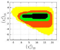
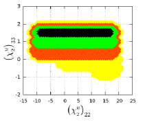
Figure 1: The allowed regions, at 90$\%$ CL, of the $\left(\widetilde{\chi}_{2}^{q}\right)_{kk}$ parameters ($k=2,3$) considering $\tan\beta=2,\,6,\,15,\,30$, yellow, orange, green and black regions respectively.

The same permitted regions for parameters space at $90\%$ CL are shown in Fig. 1.

$90<\mu_{H^{+}}<500\,\textrm{GeV}$	$\tan\beta=2$	$\tan\beta=6$	$\tan\beta=15$	$\tan\beta=30$
$\left(\widetilde{\chi}_{2}^{u}\right)_{11}$	$\left[-3.92,18\right]$	$\left[0.22,18\right]$	$\left[1.58,18\right]$	$\left[3.76,18\right]$
$\left(\widetilde{\chi}_{2}^{u}\right)_{22}$	$\left[-4.42,17.72\right]$	$\left[-1.50,17.68\right]$	$\left[0.50,17.46\right]$	$\left[2.84,16.24\right]$
$\left(\widetilde{\chi}_{2}^{u}\right)_{33}$	$\left[-0.84,1.98\right]$	$\left[-0.04,1.68\right]$	$\left[0.84,1.46\right]$	$\left[1.06,7.2\right]$
$\left(\widetilde{\chi}_{2}^{d}\right)_{11}$	$\left[-2.74,18\right]$	$\left[0.24,18\right]$	$\left[3.6,18\right]$	$\left[5.78,18\right]$
$\left(\widetilde{\chi}_{2}^{d}\right)_{22}$	$\left[-2.66,18.4\right]$	$\left[0.82,18.32\right]$	$\left[2.3,17\right]$	$\left[4.7,15.72\right]$
$\left(\widetilde{\chi}_{2}^{d}\right)_{33}$	$\left[-7.68,4.22\right]$	$\left[-2.28,2.44\right]$	$\left[-0.45,1.38\right]$	$\left[0.02,1.0\right]$
$\chi^{2}_{u}\left(\chi^{2}_{d}\right)$	$1\left(0.21\right)$	$1.17\left(0.30\right)$	$1.26\left(0.50\right)$	$1.38\left(0.78\right)$

Table 1: Average values of $\left(\widetilde{\chi}_{2}^{q}\right)_{kk}$ parameters ($k=1,2,3$) in the range $90<m_{H^{\pm}}<500\,\textrm{GeV}$, when the $\chi^{2}$-fit of Yukawa matrices is implemented.

4 Conclusions

In conclusion, we have presented the correlations between the Yukawa matrices in the framework of the 2HDM, originating from a four-zero Yukawa texture, and the current data on the CKM matrix through a $\chi^{2}$ fit. Firstly, we presented the diagonalisation of the Yukawa matrices, eventually showing that the Cheng and Sher ansatz is a particular case of our general study. Secondly, we have performed a numerical analysis via a $\chi^{2}$ fit to the Yukawa matrices with respect to the measured entries of the CKM matrix. As a consequence, we have obtained bounds for the parameters of the Yukawa texture, in particular for its diagonal terms. We have obtained results that are in complete agreement with the bounds obtained in our previous work in which we studied the flavour-violating constraints. As an outlook, we deem our current parameterisation a more easily implementable one with respect to our previous ones, thus we recommend its use for numerical analyses.

References

References

- [1] G. Aad, et al., Observation of a new particle in the search for the Standard Model Higgs boson with the ATLAS detector at the LHC, Phys.Lett. B716 (2012) 1–29. arXiv:1207.7214, doi:10.1016/j.physletb.2012.08.020.
- [2] S. Chatrchyan, et al., Observation of a new boson at a mass of 125 GeV with the CMS experiment at the LHC, Phys.Lett. B716 (2012) 30–61. arXiv:1207.7235, doi:10.1016/j.physletb.2012.08.021.
- [3] S. Chatrchyan, et al., Observation of a new boson with mass near 125 GeV in pp collisions at = 7 and 8 TeV, JHEP 1306 (2013) 081. arXiv:1303.4571, doi:10.1007/JHEP06(2013)081.
- [4] S. Glashow, Partial Symmetries of Weak Interactions, Nucl.Phys. 22 (1961) 579–588. doi:10.1016/0029-5582(61)90469-2.
- [5] S. Weinberg, A Model of Leptons, Phys.Rev.Lett. 19 (1967) 1264–1266. doi:10.1103/PhysRevLett.19.1264.
- [6] A. Salam, Weak and Electromagnetic Interactions, Conf.Proc. C680519 (1968) 367–377.
- [7] V. D. Barger, J. Hewett, R. Phillips, New constraints on the charged Higgs sector in two Higgs doublet models, Phys.Rev. D41 (1990) 3421–3441. doi:10.1103/PhysRevD.41.3421.
- [8] J. F. Gunion, H. E. Haber, G. L. Kane, S. Dawson, The Higgs hunter’s guide, Front.Phys. 80 (2000) 1–448.
- [9] M. Aoki, S. Kanemura, K. Tsumura, K. Yagyu, Models of Yukawa interaction in the two Higgs doublet model, and their collider phenomenology, Phys.Rev. D80 (2009) 015017. arXiv:0902.4665, doi:10.1103/PhysRevD.80.015017.
- [10] H. Haber, G. L. Kane, T. Sterling, The Fermion Mass Scale and Possible Effects of Higgs Bosons on Experimental Observables, Nucl.Phys. B161 (1979) 493. doi:10.1016/0550-3213(79)90225-6.
- [11] L. J. Hall, M. B. Wise, FLAVOR CHANGING HIGGS - BOSON COUPLINGS, Nucl.Phys. B187 (1981) 397. doi:10.1016/0550-3213(81)90469-7.
- [12] J. F. Donoghue, L. F. Li, Properties of Charged Higgs Bosons, Phys.Rev. D19 (1979) 945. doi:10.1103/PhysRevD.19.945.
- [13] R. M. Barnett, G. Senjanovic, L. Wolfenstein, D. Wyler, IMPLICATIONS OF A LIGHT HIGGS SCALAR, Phys.Lett. B136 (1984) 191. doi:10.1016/0370-2693(84)91179-1.
- [14] R. M. Barnett, G. Senjanovic, D. Wyler, TRACKING DOWN HIGGS SCALARS WITH ENHANCED COUPLINGS, Phys.Rev. D30 (1984) 1529. doi:10.1103/PhysRevD.30.1529.
- [15] Y. Grossman, Phenomenology of models with more than two Higgs doublets, Nucl.Phys. B426 (1994) 355–384. arXiv:hep-ph/9401311, doi:10.1016/0550-3213(94)90316-6.
- [16] A. Akeroyd, Nonminimal neutral Higgs bosons at LEP-2, Phys.Lett. B377 (1996) 95–101. arXiv:hep-ph/9603445, doi:10.1016/0370-2693(96)00330-9.
- [17] A. Akeroyd, Fermiophobic and other nonminimal neutral Higgs bosons at the LHC, J.Phys. G24 (1998) 1983–1994. arXiv:hep-ph/9803324, doi:10.1088/0954-3899/24/11/001.
- [18] A. Akeroyd, W. J. Stirling, Light charged Higgs scalars at high-energy e+ e- colliders, Nucl.Phys. B447 (1995) 3–17. doi:10.1016/0550-3213(95)00173-P.
- [19] E. Ma, Utility of a Special Second Scalar Doublet, Mod.Phys.Lett. A23 (2008) 647–652. arXiv:0802.2917, doi:10.1142/S0217732308026649.
- [20] E. Ma, Verifiable radiative seesaw mechanism of neutrino mass and dark matter, Phys.Rev. D73 (2006) 077301. arXiv:hep-ph/0601225, doi:10.1103/PhysRevD.73.077301.
- [21] R. Barbieri, L. J. Hall, V. S. Rychkov, Improved naturalness with a heavy Higgs: An Alternative road to LHC physics, Phys.Rev. D74 (2006) 015007. arXiv:hep-ph/0603188, doi:10.1103/PhysRevD.74.015007.
- [22] L. Lopez Honorez, E. Nezri, J. F. Oliver, M. H. Tytgat, The Inert Doublet Model: An Archetype for Dark Matter, JCAP 0702 (2007) 028. arXiv:hep-ph/0612275, doi:10.1088/1475-7516/2007/02/028.
- [23] S. L. Glashow, S. Weinberg, Natural Conservation Laws for Neutral Currents, Phys.Rev. D15 (1977) 1958. doi:10.1103/PhysRevD.15.1958.
- [24] A. Pich, P. Tuzon, Yukawa Alignment in the Two-Higgs-Doublet Model, Phys.Rev. D80 (2009) 091702. arXiv:0908.1554, doi:10.1103/PhysRevD.80.091702.
- [25] Y.-F. Zhou, Texture of Yukawa coupling matrices in general two Higgs doublet model, J.Phys. G30 (2004) 783–792. arXiv:hep-ph/0307240, doi:10.1088/0954-3899/30/6/008.
- [26] S. Kanemura, T. Ota, K. Tsumura, Lepton flavor violation in Higgs boson decays under the rare tau decay results, Phys.Rev. D73 (2006) 016006. arXiv:hep-ph/0505191, doi:10.1103/PhysRevD.73.016006.
- [27] S. Kanemura, K. Matsuda, T. Ota, T. Shindou, E. Takasugi, et al., Search for lepton flavor violation in the Higgs boson decay at a linear collider, Phys.Lett. B599 (2004) 83–91. arXiv:hep-ph/0406316, doi:10.1016/j.physletb.2004.08.024.
- [28] J. Hernandez-Sanchez, L. Lopez-Lozano, R. Noriega-Papaqui, A. Rosado, Couplings of quarks in the Partially Aligned 2HDM with a four-zero texture Yukawa matrix, Phys.Rev. D85 (2012) 071301. arXiv:1106.5035, doi:10.1103/PhysRevD.85.071301.
- [29] T. Cheng, M. Sher, Mass Matrix Ansatz and Flavor Nonconservation in Models with Multiple Higgs Doublets, Phys.Rev. D35 (1987) 3484. doi:10.1103/PhysRevD.35.3484.
- [30] H. Fritzsch, Calculating the Cabibbo Angle, Phys.Lett. B70 (1977) 436. doi:10.1016/0370-2693(77)90408-7.
- [31] H. Fritzsch, Z.-z. Xing, Four zero texture of Hermitian quark mass matrices and current experimental tests, Phys.Lett. B555 (2003) 63–70. arXiv:hep-ph/0212195, doi:10.1016/S0370-2693(03)00048-0.
- [32] J. Diaz-Cruz, R. Noriega-Papaqui, A. Rosado, Measuring the fermionic couplings of the Higgs boson at future colliders as a probe of a non-minimal flavor structure, Phys.Rev. D71 (2005) 015014. arXiv:hep-ph/0410391, doi:10.1103/PhysRevD.71.015014.
- [33] J. Diaz-Cruz, J. Hernandez-Sanchez, S. Moretti, R. Noriega-Papaqui, A. Rosado, Yukawa Textures and Charged Higgs Boson Phenomenology in the 2HDM-III, Phys.Rev. D79 (2009) 095025. arXiv:0902.4490, doi:10.1103/PhysRevD.79.095025.
- [34] J. Barradas Guevara, F. Cazarez Bush, A. Cordero Cid, O. Felix Beltran, J. Hernandez Sanchez, et al., Implications of Yukawa Textures in the decay within the 2HDM-III, J.Phys. G37 (2010) 115008. arXiv:1002.2626, doi:10.1088/0954-3899/37/11/115008.
- [35] M. Gomez-Bock, R. Noriega-Papaqui, Flavor violating decays of the Higgs bosons in the THDM-III, J.Phys. G32 (2006) 761–776. arXiv:hep-ph/0509353, doi:10.1088/0954-3899/32/6/002.
- [36] J. Hernandez-Sanchez, C. Honorato, M. Perez, J. Toscano, The processes in the type-III two-Higgs-doublet model, Phys.Rev. D85 (2012) 015020. arXiv:1108.4074, doi:10.1103/PhysRevD.85.015020.
- [37] J. Hernandez-Sanchez, S. Moretti, R. Noriega-Papaqui, A. Rosado, Off-diagonal terms in Yukawa textures of the Type-III 2-Higgs doublet model and light charged Higgs boson phenomenology, JHEP 1307 (2013) 044. arXiv:1212.6818, doi:10.1007/JHEP07(2013)044.
- [38] J. Hernandez-Sanchez, S. Moretti, R. Noriega-Papaqui, A. Rosado, Update of the 2HDM-III with a four-zero texture in the Yukawa matrices and phenomenology of the charged Higgs Boson, PoS CHARGED2012 (2012) 029. arXiv:1302.0083.
- [39] A. Crivellin, A. Kokulu, C. Greub, Flavor-phenomenology of two-Higgs-doublet models with generic Yukawa structure, Phys.Rev. D87 (2013) 094031. arXiv:1303.5877, doi:10.1103/PhysRevD.87.094031.
- [40] G. Branco, P. Ferreira, L. Lavoura, M. Rebelo, M. Sher, et al., Theory and phenomenology of two-Higgs-doublet models, Phys.Rept. 516 (2012) 1–102. arXiv:1106.0034, doi:10.1016/j.physrep.2012.02.002.
- [41] K. T. Haruo Yanai, Y. Takane, Projection Matrices, Generalized Inverse Matrices and Singular Value Decomposition, Springer New York Dordrecht Heidelberg London, New York, 2011.
-
[42]
J. Beringer, et al ,
Review of particle
physics, Phys. Rev. D 86 (2012) 010001.
doi:10.1103/PhysRevD.86.010001.
URL http://link.aps.org/doi/10.1103/PhysRevD.86.010001 - [43] J. Barranco, F. González Canales, A. Mondragón, Universal Mass Texture, CP violation and Quark-Lepton Complementarity, Phys.Rev. D82 (2010) 073010. arXiv:1004.3781, doi:10.1103/PhysRevD.82.073010.
- [44] F. González Canales, A. Mondragón, M. Mondragón, U. J. Saldaña Salazar, L. Velasco-Sevilla, Quark sector of S3 models: classification and comparison with experimental data, Phys.Rev. D88 (2013) 096004. arXiv:1304.6644, doi:10.1103/PhysRevD.88.096004.
- [45] A. Mondragon, E. Rodriguez-Jauregui, The Breaking of the flavor permutational symmetry: Mass textures and the CKM matrix, Phys.Rev. D59 (1999) 093009. arXiv:hep-ph/9807214, doi:10.1103/PhysRevD.59.093009.
- [46] F. González Canales, A. Mondragón, M. Mondragón, The Flavour Symmetry: Neutrino Masses and MixingsarXiv:1205.4755.
- [47] Z.-z. Xing, H. Zhang, S. Zhou, Updated Values of Running Quark and Lepton Masses, Phys.Rev. D77 (2008) 113016. arXiv:0712.1419, doi:10.1103/PhysRevD.77.113016.
- [48] K. Chetyrkin, J. H. Kuhn, M. Steinhauser, RunDec: A Mathematica package for running and decoupling of the strong coupling and quark masses, Comput.Phys.Commun. 133 (2000) 43–65. arXiv:hep-ph/0004189, doi:10.1016/S0010-4655(00)00155-7.
- [49] F. González Canales, A. Mondragón, U. S. Salazar, L. Velasco-Sevilla, as a unified family theory for quarks and leptonsarXiv:1210.0288.
- [50] A. Cordero-Cid, J. Hernandez-Sanchez, C. Honorato, S. Moretti, M. Perez, et al., Impact of a four-zero Yukawa texture on and in the framework of the Two Higgs Doublet Model Type III, JHEP 1407 (2014) 057. arXiv:1312.5614, doi:10.1007/JHEP07(2014)057.