On the quality of complementary bounds for eigenvalues
Abstract
A concrete formulation of the Lehmann-Maehly-Goerisch method for semi-definite self-adjoint operators with compact resolvent is considered. Precise rates of convergence are determined in terms of how well the trial spaces capture the spectral subspace of the operator. Optimality of the choice of a shift parameter which is intrinsic to the method is also examined. The main theoretical findings are illustrated by means of a few numerical experiments involving one-dimensional Schrödinger operators.
Keywords. Lehmann-Maehly-Goerisch method, Zimerman-Mertins method, eigenvalue computation, complementary eigenvalue bounds.
1 Introduction
The neat formulation by Zimmermann and Mertins [22] (see also [8, Section 6]) of the Lehmann-Maehly-Goerisch method [10, 9, 13, 14, 15] (see also [21, Chapter 4.11]), has recently shown to be a reliable tool for computing eigenvalue enclosures [4, 8, 3, 6, 2, 1]. In its most basic framework, this formulation involves fixing a “shift” parameter and then characterising the spectrum which is adjacent to by means of a combination of the Variational Principle with the Spectral Mapping Theorem.
The present paper is devoted to re-examining this most basic setting for semi-definite self-adjoint operators with a compact resolvent. Two main contributions are to be highlighted. On the one hand, we determine how the choice of affects the quality of the eigenvalue bound. On the other hand, we establish explicit convergence estimates, in terms of how well spectral subspaces in a neighbourhood of are captured by the underlying trial subspaces. The latter is closely linked with a similar convergence analysis pursued in [5] for the so-called quadratic method.
In addition to these theoretical contributions, we apply our findings in the detailed study of a concrete model. For this purpose we consider computation of upper and lower bounds for the eigenvalues of one-dimensional Schrödinger operators with potential singular at infinity by means of the finite element method. Similar ideas have been realised for the Helmholtz equation [4], calculation of sloshing frequencies [3] and the MHD operator [6]. See also the recent manuscripts [2] and [1].
The first part of the paper is concerned with the abstract theory. Section 2 is devoted to a formulation of the most basic framework in the approach described in [22]. In Section 3 we determine how the choice of the parameter affects the quality of the eigenvalue bounds (Theorem 3.2). Properties of convergence are then established in Section 4. Our main contribution in this respect is summarised by Theorem 4.4.
The second part of the paper is devoted to the concrete model. Section 5 describes how to discretise the Schrödinger operator by means of the finite element method. There we establish precise convergence rates in this particular case. In Section 6 we include various computational experiments performed on the harmonic and the anharmonic oscillators.
Notation
Everywhere below denotes a Hilbert space with inner product and norm . The self-adjoint operator , will always be assumed to be semi-bounded below and its resolvent operator
will be assumed to be compact for one and hence all outside the spectrum. Under these hypotheses, the spectrum of , , is always an increasing sequence of isolated eigenvalues of finite multiplicity accumulating at . We will write
counting multiplicities with the index.
Here, and everywhere else in this paper, will denote a real parameter. We will often leave implicit the dependence of some of the -dependant quantities, whenever this is sufficiently clear from the context. This will be so the case especially in the proofs of some of the main statements.
For , we will write
so that and . In general,
are closed quadratic forms, but this is not necessarily the case for on . Moreover defines a Hilbert space if and only if . We will occasionally write .
Let be a given subspace of dimension such that
for a suitable linearly independent set . We will write
2 Complementary eigenvalue bounds
The most basic setting of the strategy established in the paper [22] can be summarised as follows. Let be fixed. In order to give certified bounds for the spectrum of in the vicinity of , we seek for the eigenvalues of the following problem: find and , such that
| (1) |
2.1 Adjacent eigenvalues
Consider the case of the eigenvalues which are immediately adjacent to , both to the left and to the right. Let be such that
Assume that is such that
| (2) |
Then (1) for and leads to upper and lower bounds for . Indeed, denote the extremal eigenvalues of (1) by
| (3) |
The following statement is a simplified version of [22, Theorem 2.4]. See also [8, Theorem 11] and Lemma 2.2 below.
Lemma 2.1.
If (2) holds true, then , and
Proof.
Condition (2) on implies immediately . Let
According to the Spectral Mapping Theorem and the Min-max Principle,
This ensures the inequality on the left hand side.
The complementary inequality and the statement for are shown analogously. ∎
2.2 Further eigenvalues
Let be the number of eigenvalues of which are below counting multiplicity. Here and elsewhere we convey in writing when , as well as .
As we shall see next, according to the Min-max Principle, the eigenvalues of below are characterised by the quantities
| (4) |
and those above are characterise by the quantities
| (5) |
The following lemma is exactly [22, Theorem 1.1]. Here and everywhere below the index will count multiplicities.
Lemma 2.2.
Let . Then
and
Proof.
Here
and is guaranteed due to the invertibility of . Therefore is the eigenvalue of which is on the th position counting multiplicities right to left from . As there are exactly eigenvalues of below , according to the Spectral Mapping Theorem, then there are exactly of these which are negative. Due to the ordering of the eigenvalues of relative to , the index on the corresponds to that of . Thus
For the other case we proceed analogously, taking into account the fact that we have infinitely many eigenvalues of above , which in turns become the positive accumulating at from the right. ∎
This statement motivates the following definition. Assume that (1) has exactly negative eigenvalues and positive eigenvalues. We will see below that whenever is sufficiently close to the eigenspace associated to . Let denote these negative eigenvalues and denote these positive eigenvalues, respectively, for .
Lemma 2.3.
For ,
| (6) |
and
| (7) |
Proof.
This follows immediately from the Min-max Principle applied to the matrix problem associated to (1). ∎
A combination of lemmas 2.3 and 2.2 leads to the following generalisation of Lemma 2.1, which is exactly the content of [22, Theorem 2.4]. See also [8, Theorem 11] and [2, Corollary 7].
Lemma 2.4.
Let . Then
| (8) |
and
| (9) |
Proof.
In view of Lemma 2.4, the inverse residuals give lower and upper bounds for the eigenvalues of which are below and above , respectively.
Remark 2.5.
In general , but it is not necessarily guaranteed that . On a practical setting, a priori information about the value of is required, if we wish to determine the correct indexing of the lower bounds for the points in which are below . This is a known limitation of the current approach, which in particular frameworks can be handled by means of homotopy methods [16, 17].
In spite of this observation, note that a positive implies the existence of eigenvalues of below .
3 Optimal choice of the shift
The quality of the bounds established in Lemma 2.4 depends on the choice of the parameter . We now examine the optimality of these bounds and show that this is achieved as moves away from the eigenvalue of interest. We begin with an auxiliary statement.
Lemma 3.1.
Let be such that . Assume that is such that either or . Then
| (10) |
Proof.
Let be as in the hypothesis. Without loss of generality we can assume that . By the Cauchy-Schwarz inequality,
Then
Hence
According to the hypothesis, either both and are positive or both are negative. Thus
∎
The following is the main statement of this section. We formulate it in terms of for a fixed value of and consider moving along . Note that the hypothesis ensures that .
Theorem 3.2.
Let and be such that
Then the following holds true.
-
1.
and
-
2.
and
Proof.
Let with be such that there exists with and
Then
for a special (maximising) vector .
Since and
then also . Hence .
Now, as both sides of the inequality above are negative, we gather that
Hence, by the definition of above, the fact that the fractions involved are negative, and an application of (10) with and , we get
Note that we can do all this for running from to . ∎
Consider the specific group of eigenvalues,
| (11) |
Suppose we find upper bounds for these eigenvalues from a fixed and lower bounds from a fixed . Denote these bounds by
If we choose and , denoting
gives
Indeed, set and for . According to Theorem 3.2,
Then
4 Convergence
We now examine the convergence of the bounds established in Lemma 2.4, in a regime where captures the eigenvectors of . Our aim will be to show that, under suitable conditions,
| (12) |
for any .
4.1 Auxiliary results
We firstly set a notation that simplifies greatly the arguments below. Let
| (13) |
and
| (14) |
(recall (4) and (5)). The quadratic forms
are positive and closed. Moreover
We write , so that are a Hilbert spaces with respect to this norm.
Let
and
Let
and
As , in order to examine the limits (12), we might as well focus on studying the convergence . Our analysis below follows closely that of the classical setting [20, §4.4 and Ch.6].
Let be the projections orthogonal in the inner products respectively. Let be a fixed family of eigenvectors such that . We assume that the are chosen to be orthonormal in the inner product of .
Let
be the eigenspace associated to the eigenvalues up to index . Set
and
| (15) |
The following lemma mimics [20, Lemma 6.1].
Lemma 4.1.
If , then .
Proof.
The above shows that necessarily for any , if the hypothesis is to be satisfied. In turns this implies that . Then,
Now since is the orthonormal projection in the inner product , then . Also
So
∎
By virtue of the previous lemma and the fact that
if is close to 0, then is close to . In the next two lemmas we set conditions for to be small.
Lemma 4.2.
Let . Then
Proof.
We only consider the proof with the “” sign, the proof with the “” sign being analogous.
For and ,
Then
So, if we expand where (recall that we are assuming ), then
The second and fourth inequalities are the Cauchy-Schwarz inequality, the third inequality is the triangle inequality. Here we are using the fact that , so that
∎
Lemma 4.3.
Let . Then
Proof.
Expand for . Then,
∎
4.2 Main statement on convergence
Theorem 4.4.
Fix a group of eigenvalues as in (11) and let
There exist a constant only dependant on , and , ensuring the validity of the following. If is such that, for any there exist such that
where
then
| (16) |
and
| (17) | ||||
Proof.
Let us show the existence of ensuring (16). That we can find a (perhaps larger) ensuring both (16) and (17), follows by means of the same technique applied to the “+” case. Firstly note that
This yields
Since
then
for a chosen constant that allows
for all . This choice ensures (16).
The arguments leading to the conclusion (17) are very similar. ∎
In the remaining parts of this paper we explore an implementation of the method introduced in Section 2 to one-dimensional Schrödinger hamiltonians under suitable conditions on the potential. These operators satisfy the hypothesis of being bounded below with a compact resolvent. The trial spaces will be taken to be generated by the finite element method. We examine the convergence properties of this implementation, in the contexts of Theorem 4.4.
5 Eigenvalue bounds for Schrödinger operators in one dimension
Let be a one-dimensional semi-definite Schrödinger operator with a compact resolvent. Let the trial subspaces be constructed via the finite element method on a large, but finite, segment. Under standard assumptions on the finite element spaces, below we determine the precise rate at which the upper and lower bounds in Lemma 2.4 converge to the true eigenvalues of , as the mesh refines and the length of the segment grows. We refer to [5, Section 4] for similar results in the context of the so-called quadratic method.
5.1 The model hamiltonian and its truncation to a finite box
Let
acting on . We assume that the potential is real-valued, continuous and as . These conditions ensure that the operator is self-adjoint on a suitable domain and it has a compact resolvent [18, Theorem XIII.67]. The domain of closure of the quadratic form associated to is
Note that this is the intersection of the maximal domains of the momentum operator and the operator of multiplication by . Here and below we denote for .
The conditions on the potential imply that for all and a suitable constant . This ensures that is bounded below, and . Without loss of generality we will assume below that .
From the fact that we are in one space dimension alongside with the condition of continuity on the potential, we know that all the eigenvalues of have multiplicity equal to 1. Moreover, the eigenfunctions are and they decay exponentially fast at infinity [19, Section C.3]. Following the notation for the generic operator above, we write
We let the orthonormal basis of be such that
Without further mention, below we often suppress the index from the eigenvalue and the eigenfunction, when it is sufficiently clear from the context.
Let . Consider the restricted operator
subject to Dirichlet boundary conditions: . As , we expect that the spectrum of approaches the spectrum of . In fact, this turns out to happen exponentially fast (in ) for individual eigenvalues, whenever is such that for every there exists a constant ensuring
(see e.g. [5, Theorem 4.4]). Without further mention, everywhere below we impose this additional assumption on the potential.
The operator is self-adjoint on a domain defined via Friedrichs’ extensions. Denote by the quadratic form associated to . Since is continuous on the whole of , then the domain of closure of is
see [12, Theorem VI.2.23 and VI.4.2].
As , the forms and are both positive definite. Hence the quantities
define norms in and respectively.
5.2 Finite element discretisation
Let be an equidistant partition of into sub-intervals of length . Let where
| (19) |
is the finite element space generated by conforming elements of order subject to Dirichlet boundary conditions. Here we require and , so that . Everywhere below we assume that these two parameters are fixed.
Let us now establish a concrete result showing that the hypothesis of Theorem 4.4 is satisfied in the present setting. In turns this will imply that, if we implement a numerical strategy for computing , this implementation is convergent.
Our first statement is [5, Theorem 4.5], but we include its proof for completeness.
Lemma 5.1.
Fix . There exist large enough and small enough, such that the following is satisfied. For and , we can always find such that
-
1.
-
2.
-
3.
where
for a suitable and constants dependant on , but independents of or .
Corollary 5.2.
Let and be fixed. There exist and large enough, and and small enough, ensuring the following. There always exists such that
for and .
Proof.
Let be as in the previous lemma. Then
This ensures the existence of the required constants.∎
Theorem 5.3.
Let . Let be as in the previous corollary. There exist constants , such that
and
In the next section we consider two models with concrete potentials and explore numerically the scope of this theorem.
6 Numerical experiments
In all the examples below we consider Hermite elements of order which are conforming, so are as in (19) with a linear combination of two basis polynomials of order 3.
As for model hamiltonians, we consider the quantum harmonic and anharmonic oscillators. Let and . The exact eigenvalues are
and the corresponding eigenfunctions are
where are the Hermite polynomial of order . Let for . In this case the exact eigenvalues and eigenfunctions are not known explicitly.
6.1 Eigenvalue bounds and order of convergence
Theorem 5.3 shows that the limits (12) are convergent at a rate proportional to in the regime and , when the trial spaces are chosen to be . In all calculation below we fix .
The eigenvalue problem (1) is equivalent to that of the matrix problem
In the numerical computations presently conducted, we have found from the solution of this linear eigenvalue problem. The coefficients of the matrices , and , were all computed analytically. See the Appendix in [5].
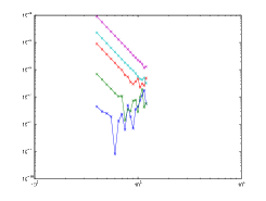
Table 1 shows approximation of five eigenvalues of and with , by means of the Galerkin method and by means of the Lehmann-Maehly-Goerisch method. The trial subspace has been taken exactly the same in both cases. The Galerkin method give certified upper bounds for . Observe that these upper bounds are roughly four orders of magnitude sharper than those obtained from an application of the Lehmann-Maehly-Goerisch method with . See Figure 4.
Remark 6.1.
Recall Remark 2.5. There is a strong indication that the numerical quantities shown in Table 1 correspond to the first five eigenvalues of . This is certainly the case for . However, without any a priori information about the position of the sixth eigenvalue (not shown), this claim cannot be made with mathematical rigour. In the numerical experiments of this section we have “abused” slightly the notation and written the index as for the eigenvalues of both and .
harmonic anharmonic 1 2 3 4 5
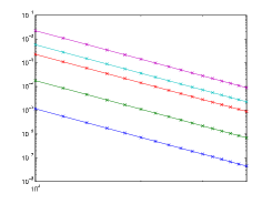
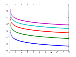
Figure 1 shows versus the size of the eigenvalue enclosure , for an upper bound found from (9) and a lower bound found from (8). In this figure the slopes are fairly close to , indicating that the convergence rates established in Theorem 5.3 are optimal.

6.2 Large trial spaces and truncation error
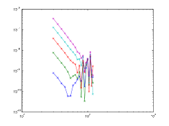
When the size of the matrices increases, the residuals shown in Figure 1 reach a threshold. After this threshold, truncation error in (finite) 16 digits precision takes over. We show this phenomenon in Figure 2. Accurate approximation of the enclosures for each individual eigenvalues for large, but chosen below this threshold, are given in Table 2.
harmonic anharmonic 1 450 550 2 500 650 3 550 750 4 650 950 5 700 1050
6.3 Influence of the shift on the eigenvalue bounds
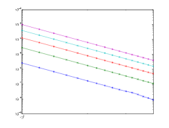
We now examine the influence of the choice of on the quality of the eigenvalue bounds, as described in Section 3. In Table 1 we fixed in order to compute the upper eigenvalue bounds and in order to compute the lower eigenvalue bounds. Figure 3 shows different choices of versus in semi-log scale. As predicted by Theorem 3.2, the further the moves away from the spectrum, the more accurate the enclosure becomes.


The Galerkin method is widely acknowledged to be the standard approach for computing upper bound for eigenvalues. See Table 1. From the illustration shown in Figure 4, it is natural to predict that the upper bounds (9) approach those provided by the Galerkin method in the regime .

Acknowledgements
Financial support was provided by the Engineering and Physical Sciences Research Council (grant number EP/I00761X/1) and King Abdulaziz University.
References
- [1] G. Barrenechea, L. Boulton, and N. Boussaïd. Finite element eigenvalue enclosures for the Maxwell operator. Preprint 2014. Available at arXiv: 1402.4911.
- [2] G. Barrenechea, L. Boulton, and N. Boussaïd. Eigenvalue enclosures. Preprint 2013. Available at arXiv:1306.5354.
- [3] H. Behnke. Lower and upper bounds for sloshing frequencies. In Inequalities and applications, volume 157 of Internat. Ser. Numer. Math., pages 13–22. Birkhäuser, Basel, 2009.
- [4] H. Behnke and U. Mertins. Bounds for eigenvalues with the use of finite elements. In Perspectives on enclosure methods (Karlsruhe, 2000), pages 119–131. Springer, Vienna, 2001.
- [5] L. Boulton and A. Hobiny. On the convergence of the quadratic method. Preprint 2013. Available at arXiv:1307.0313.
- [6] L. Boulton and M. Strauss. Eigenvalue enclosures and convergence for the linearized MHD operator. BIT, 52(4):801–825, 2012.
- [7] P. Ciarlet, The finite element method for elliptic problems, North-Holland, Amsterdam, 1978.
- [8] E. B. Davies and M. Plum. Spectral pollution. IMA J. Numer. Anal., 24(3):417–438, 2004.
- [9] F. Goerisch. Eine Verallgemeinerung eines Verfahrens von N. J. Lehmann zur Einschließung von Eigenwerten. Wiss. Z. Tech. Univ. Dres., 29:429–431, 1980.
- [10] F. Goerisch and H. Haunhorst. Eigenwertschranken für Eigenwertaufgaben mit partiellen Differentialgleichungen. Z. Angew. Math. Mech., 65(3):129–135, 1985.
- [11] T. Kato. On the upper and lower bounds of eigenvalues. J. Phys. Soc. Japan, 4:334–339, 1949.
- [12] T. Kato. Perturbation theory for linear operators, volume 132. Springer Verlag, 1995.
- [13] N. J. Lehmann. Beiträge zur numerischen Lösung linearer Eigenwertprobleme. Parts I. Z. Angew. Math. Mech., 29:341–356, 1949.
- [14] N. J. Lehmann. Beiträge zur numerischen Lösung linearer Eigenwertprobleme. Parts II. Z. Angew. Math. Mech., 30:1–6, 1950.
- [15] H. J. Maehly. Ein neues Verfahren zur gendherten Berechnung der Eigenwerte hermitescher Operatoren. Helv. Phys. Acta, 25:547–568, 1952.
- [16] M. Plum. Bounds for eigenvalues of second-order elliptic differential operators. ZAMP, 42:848–863, 1991.
- [17] M. Plum. Eigenvalue inclusions for second-order ordinary differential operators by a numerical homotopy method. ZAMP, 41:205–226, 1990.
- [18] M. Reed and B. Simon. Methods of modern mathematical physics. IV. Analysis of operators. Academic Press, New York, 1978.
- [19] B. Simon. Schrödinger semigroups. Bull. Amer. Math. Soc. (N.S.), 7(3):447–526, 1982.
- [20] G. Strang and G. Fix. An analysis of the finite element method. Wellesley-Cambridge Press, Wellesley, second edition, 2008.
- [21] H. F. Weinberger. Variational Methods for Eigenvalue Approximation. SIAM, Philadelphia, 1974.
- [22] S. Zimmermann and U. Mertins. Variational bounds to eigenvalues of self-adjoint eigenvalue problems with arbitrary spectrum. Z. Anal. Anwendungen, 14(2):327–345, 1995.