X-ray time delays in the Narrow Line Seyfert 1 galaxy PG 1244+026

Abstract

We analyse the X-ray time-lags in the Narrow Line Seyfert 1 (NLS1) galaxy PG 1244+026 ($M_{\rm BH}\sim 10^{7}\hbox{$\thinspace M_{\odot}$}$, $L/L_{\rm Edd}\sim 1$). The time delay between the soft (0.3–0.7 keV) and harder (1.2–4.0 keV) variations shows shows the well established switch from hard lags at low frequencies to soft lags at high frequencies. The low frequency hard lags are qualitatively consistent with the propagation of fluctuations model, with some long-timescale response of the reflection component. The high frequency soft lag appears to extend over a wide frequency band, that we divide this into two narrow frequency ranges, and examine the lag as a function of energy for each of these. At high frequencies the soft excess emission is delayed with respect to the harder energy bands, without any corresponding strong, hard X-ray reflection signature. At even higher frequencies a soft lag is seen at the softest energies, as well as tentative evidence for an iron K$\alpha$ reverberation signal. These results point to the importance of reprocessing as well as reflection in determining the lags in NLS1s.

1 Introduction

The X-ray spectra of AGN usually show a soft X-ray excess (hereafter, soft excess) above the low energy extrapolation of the 2-10 keV power law emission. The shape of this soft excess is often equally well modelled by either smeared, ionised reflection (presumably from the surface of the putative accretion disc: Crummy et al. 2006; Walton et al. 2013) or by a separate soft continuum component (Vaughan et al. 2002; Gierliński & Done 2004). X-ray spectral fitting alone cannot distinguish between these quite smooth spectral models given the typically bandpass available to X-ray observatories.

Studies of X-ray variability can give complementary information, potentially breaking this deadlock. The X-ray reflection model predicts time delays between variations in the primary continuum, and the reflected response of the disc (Stella 1990; Reynolds 1999). The primary features of a disc reflected spectrum include fluorescence/resonance line emission, particularly from iron, and a curved continuum at high energies. The signal-to-noise around the $\sim 6.4$ keV Fe K$\alpha$ line is often rather low, but if the disc surface is moderately ionised there could also be strong soft X-ray emission (e.g. Ross & Fabian 2005), and this soft emission will also lag behind the illuminating continuum. However, these lags are simply the light travel time to the reflector, so should be short ($10R_{\rm g}/c\sim 500$ seconds for $M_{\rm BH}=10^{7}M_{\odot}$) so are best probed by the fastest variability. Concentrating on fast variability is also necessary as accreting black holes (BHs) seem to display hard lags at low frequencies — slow variations in the hard energy bands are delayed with respect to the soft energy bands (Miyamoto & Kitamoto 1989; Nowak et al. 1999a; 1999b; Vaughan et al. 2003a; 2003b; McHardy et al. 2004). The favoured model for the origin of hard lags is the radial propagation of accretion rate fluctuations through a stratified emission region (e.g. Kotov et al. 2001, Arévalo & Uttley 2006). In combination, these two effects predict a switch from hard (propagation) lags at lower frequencies to soft (reflection) lags at higher frequencies. This pattern was tentatively observed in McHardy et al. (2007), and has now been observed in $\sim 20$ AGN (e.g. Fabian et al. 2009; Emmanoulopoulos et al. 2011; Zoghbi & Fabian 2011; Alston et al. 2013; Cackett et al. 2013; De Marco et al. 2013; Kara et al. 2013), and one black hole X-ray binary (XRB; Uttley et al. 2011).

Narrow Line Seyfert 1 galaxies (NLS1s) are the targets of choice for much of this work as they are typically brighter in soft X-rays, and have low black hole mass, so their variability timescales are the shortest amongst AGN, so they can be studied more easily in single observations at high signal-to-noise. A subset of NLS1s (the ‘complex’ NLS1s: Gallo 2006) can also show much more dramatic variability than seen in broad line Seyfert 1s (BLS1s), with deep dips in their X-ray light curves where their spectra appear dominated by reflection (Fabian et al. 2004; 2009). Hence these should give the clearest detections of reverberation lags, contrasting with the ‘simple’ NLS1, which show only moderate reflection and variability amplitude Gallo 2006. NLS1s typically show stronger soft excesses than broad line AGN (e.g. Boller et al. 1996; Middleton et al. 2007), so the soft lag signature should be strong in all these systems if the soft excess is from reflection. However, detailed spectral decomposition shows that the majority of the strong soft X-ray emission in NLS1s can be attributed to direct emission from the accretion disc, itself extending into the soft X-ray bandpass. There is still a ‘true’ soft excess (which can again be made from either ionised reflection or an additional component) in addition to the disc and coronal components, but it is actually smaller than in broad line objects (Jin et al. 2012a; 2012b; Done et al. 2012; Jin et al. 2013; hereafter J13).

J13 used frequency resolved spectroscopy (e.g. Revnivtsev et al. 1999) as another approach to study the origin of the ‘true’ soft excess in the ‘simple’ NLS1 PG 1244+026 . The fastest variability (timescales $\leq 5000$ s) has a spectrum in which the soft excess is less prominent than in the time averaged spectrum, as expected if the corona is closest to the black hole so has more rapid variability than the soft excess and disc emission (J13). However, little of this rapid variability of the soft excess is correlated with the 3-10 keV light curve. This seems to rule out an ionised reflection origin for the majority of the soft excess, since ionised reflection produces simultaneously the soft excess and the Fe K$\alpha$ line and reflection continuum at higher energies (J13).

In this paper we explore the time lags from PG 1244+026  as a function of Fourier frequency and of energy.

2 Observations and data reduction

PG 1244+026 was observed by XMM-Newton for $\sim 123$ ks in December 2011 (OBS ID: 0675320101). The timing analysis in this paper uses data from the EPIC-pn camera (Strüder et al., 2001) only, due to its higher throughput and time resolution. The pn data were taken in small window (SW) mode, which reduces the impact of event pile-up (Ballet 1999; Davis 2001). The raw data were processed from Observation Data Files following standard procedures using the XMM-Newton Science Analysis System (sas v13.0.0) with a 20 arcsec circular extraction region. Regions with high background were filtered from the data, but these are very minor, and there was no sharp rise in background towards the end of the observation.

3 Lag as a function of frequency

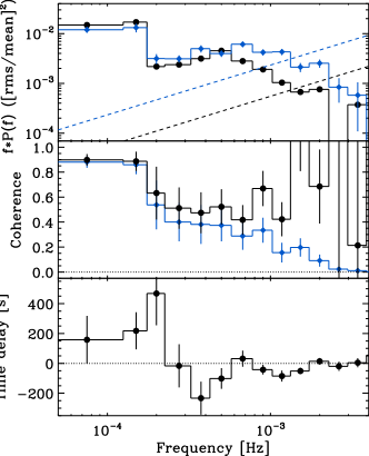
Figure 1: Cross-spectral products for the soft (0.3–0.7 keV) and hard (1.2–4.0 keV) energy bands. Panel (a) shows power spectral density for the soft (black circles) and hard (blue diamonds) bands. The dashed lines are the Poisson noise estimates. Panel (b) shows the raw (blue diamonds) and Poisson noise corrected (black circles) coherence, see section 3 for details. Panel (c) shows the time lag between the hard and soft band, where a positive values indicate the hard band lags.

3.1 The observed lag-frequency

In this section we explore the cross-spectral products between a soft and hard band. We use 0.3–0.7 keV as a soft band to maximise the disc and soft excess components, with little contamination from the hard X-ray coronal emission, and 1.2-4 keV as a hard band to maximise the coronal emission, with little contamination from the soft excess or reflected iron K$\alpha$ emission (J13, see also Fig. 5). These bands have mean count rates of 5.8 and 0.8 $\mathrm{ct\,s}^{-1}$ respectively.

We compute cross spectra following e.g. Vaughan & Nowak (1997); Nowak et al. (1999); Vaughan et al. (2003). We estimated cross-spectral products by first calculating complex cross-spectra values in $M$ non-overlapping segments of time series, and then averaging over the $M$ estimates at each Fourier frequency. We then averaged in geometrically spaced frequency bins (each bin spanning a factor $\sim 1.3$ in frequency). For the analysis in this paper we use segment sizes of 20 ks and time bins of 20 s, leaving 6 segments in total. The choice of segment length and frequency bin averaging was chosen to maximise the number of data points being averaged in the cross-spectrum, whilst still maintaining a high enough frequency resolution to pick out any features in the cross-spectral products.

The upper panel in Fig. 1 shows the Poisson noise subtracted power spectra for the hard (blue) and soft (black) bands. These are very similar to those in J13 and are only given here for completeness. The Poisson noise level is estimated using equation A2 of Vaughan et al. (2003), and is indicated by the dashed lines.

From the cross-spectra we get the coherence between the hard and soft band (e.g. Bendat & Piersol 1986). The coherence is defined between [0,1], where 1 is perfect coherence and 0 is perfect incoherence. This gives an estimate of the linear correlation between the two bands, i.e. how much of the variability in one band can be linearly predicted by the other. The middle panel of Fig. 1 shows the ‘raw’ coherence (blue) and the coherence after Poisson noise correction (black), following Vaughan & Nowak (1997). The noise corrected coherence is high ($\sim 0.9$) for frequencies up to $\sim 1.5\times 10^{-4}$ Hz, showing that soft and hard band variations are very well correlated on timescales longer than a few ks, but then drops to $\sim 0.5$ between $\sim 1.5-10\times 10^{-4}$ Hz, and becomes well correlated again at frequencies higher than $\sim 1.5\times 10^{-3}$ Hz.

From the cross-spectrum we also obtain a phase lag at each frequency, $\phi(f)$, which we transform into the corresponding time lag $\tau(f)=\phi(f)/(2\pi f)$ with errors estimated using raw coherence (Vaughan & Nowak 1997; Bendat & Piersol 1986). We checked this method produces reliable error estimates when the contribution of Poisson noise is large using Monte Carlo simulations (see e.g. Alston et al. 2013). The lower panel shows these frequency dependent time lags between the soft and hard bands, where we follow convention by using a negative time lag to indicate the soft band lagging behind the hard band (hereafter ‘soft lags’).

The lag-frequency spectrum shows a hard lag at frequencies below $\approx 2\times 10^{-4}$ Hz, whereas between $\approx 3\times 10^{-4}$ and $2\times 10^{-3}$ the soft emission lags the hard, with a maximum soft lag of $\sim 250$ s at $\sim 4\times 10^{-4}$ Hz. This shape is similar to that seen in other sources, and seems to be quite common in low-redshift, X-ray variable AGN (e.g. Fabian et al. 2009; Emmanoulopoulos et al. 2011; De Marco et al. 2013).

3.2 Modelling the lag-frequency

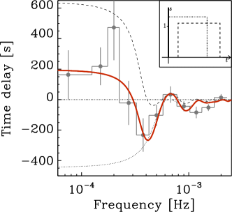
Figure 2: The Top hat—Top hat model fit to the lag-frequency spectrum. The red solid line is the model fit integrated over the frequency bin, matching the fitting procedure. The dashed and dotted lines show the individual transfer functions in each band. The inset illustrates the top hat and $\delta$-function responses in each band. See Sec. 2 for details.

In this section we model the lag-frequency spectra using simple analytical models. Following the approach of Alston et al. (2013) (and references therein) we use a top hat response functions (or transfer functions when discussing the response function in the Fourier domain), as well as a power-law dependence on lag-frequency, to model the frequency dependent time delays. The response functions can be present in either the hard band, the soft band or both, together with a $\delta$-function response to account for direct (unreprocessed) emission. The difference between these two (actually, the complex argument of the product of the two complex transfer functions, see Alston et al. 2013) predicts the lag-frequency data between the two bands. We fit the lag-frequency data using standard $\min(\chi^{2})$ fitting techniques, integrating the model over the bin width, rather than fitting just at the bin centre.

A roughly power-law frequency dependence of the hard X-ray time lag is well established in X-ray binaries (e.g. Miyamoto et al. 1988; Nowak et al. 1999; Pottschmidt et al. 2000), at least at low frequencies, and consistent results from AGN have been reported several times (e.g. Papadakis et al. 2001; Vaughan et al. 2003; McHardy et al. 2004; Arévalo et al. 2006). We therefore consider a power-law model of the form $\tau(f)=Nf^{-\alpha}$ with $\alpha\approx 1$. However, a power-law response function alone (with no $\delta$-function) for the hard band gives an unacceptable fit to the lag-frequency data ($p<10^{-8}$), as this predicts only positive (hard) lags.

We next model the response of the system assuming a $\delta$ function in the soft band, and a $\delta$ function plus a top hat in the hard band. The $\delta$ functions represent the non-delayed continuum emission in each band. A $\delta$ function plus top hat is clearly just an approximation to a more complex response function, but is relatively simple to fit and allows for comparison with previous work in this area. The parameters of the top hat are start time $t_{0}$, width $w$ and area $S$ (which sets the intensity of delayed emission relative to the direct emission). This was used to model distant reflection by Miller et al. (2010), but the physical picture here is that it models the propagation time delays, as there is probably little reflection contributing to our ‘hard’ (1.2-4 keV) bandpass (see Alston et al. 2013, J13). However, irrespective of the way this is interpreted, this can reproduce both positive and negative lags from ‘ringing’ in the Fourier domain as a result of the sharp edges of the impulse response function (Miller et al., 2010). This model also gives a poor fit to the data ($p\sim 10^{-4}$) as the resulting negative lag from ringing is too sharp to explain the broad frequency range of the observed soft lag (see also Zoghbi et al. 2011; Emmanoulopoulos et al. 2011).

We next considered models including an additional top hat response in the soft band response, where this soft top hat is now physically modelling a reverberation response to the direct emission, whereas the top hat in the hard band is modelling propagation lags. Thus the total model is a $\delta$ function plus top hat in both hard and soft bands, giving a total of 6 free parameters (3 for each top hat). We find a good fit to the data with $\chi^{2}$ = 9 / 5 d.o.f ($p=0.1$). The full resolution model is shown as the red solid line (Fig. 2). The hard response parameters are: $t_{0}^{h}=330\pm 80{\rm s}$, $w^{h}=1780\pm 220{\rm s}$, and $S^{h}=1.1\pm 0.3$, while the soft response parameters are: $t_{0}^{s}=0\pm 100{\rm s}$, width $w^{s}=1520\pm 140{\rm s}$, and scaling fraction $S^{s}=1.4\pm 0.5$.

The lags due to any one component of the combined model can be isolated by computing the lag-frequency curve assuming that the response function in the other band is simply a $\delta$ function. If the soft band response is replaced by a $\delta$ function then the top hat in the hard causes the hard band variations to lag the soft band variations (dashed line). Conversely if the hard band response is replaced by a $\delta$ function then the top hat in the soft band causes the soft to lag the hard (dotted line), but the soft lag extends to higher frequencies due to the narrower width of the top hat in the soft band than in the hard. The lags measured between the two bands, as a function of frequency, is a combination of these lags on each band which may be operating in different directions and so partially cancelling out. The lag from the combined model is approximately the sum of the lag contributions from each model component (these two are not in general exactly equal as the phase difference between two transfer functions is computed after averaging the real and imaginary components of each transfer function over the finite frequency bins).

The typical propagation lags of the hard band behind the soft band are $\sim 1000$ s, while the typical reverberation timescale lags of the soft band behind the hard band are of order $\sim 750$ s. It is this timescale which gives the size scale of the reprocessor, not the lag of $\sim 250$ seconds as given from the cross-spectrum as the latter does not include the effect of dilution of the lagged flux (top hat) by the direct flux ($\delta$ function) (see e.g. Miller et al. 2010; Wilkins & Fabian 2013a). Hence the reprocessing typically occurs on size scales of $15R_{\rm g}$ for a black hole mass of $10^{7}$$\thinspace M_{\odot}$.

We note that the model still does not quite match the soft lags observed at the highest frequencies. We could improve the fit by adding another top hat in the soft band, starting from $t_{0}^{s2}=0$ with width of $\sim$ few hundred seconds. This would skew the response more towards shorter timescales i.e. to weight the reverberation towards smaller distance material. Given the limited frequency resolution, such a complex model will over-fit the data. We note that improvement in fitting the highest frequency soft lags may also be achieved with the use of ‘realistic’ response function, rather than a simple top hat plus $\delta$ function in the soft band (e.g. Campana & Stella 1995; Reynolds 2000; Wilkins & Fabian 2013b).

4 The frequency resolved lag-energy spectrum

4.1 The observed lag-energy spectra

A lag-energy spectrum can be calculated over a given range in frequency by estimating the cross-spectral lag between a light curve in each energy band with respect to the frequency resolved light curve over a broad reference band (e.g. Zoghbi et al. 2011). We take our reference band as the hard band in the previous lag-frequency work i.e. the 1.2–4.0 keV light curve minus the energy band for which the lag is being computed so that we never have correlated Poisson noise. This reference band is chosen to maximise the lags between the coronal emission and the soft excess and reflected iron K$\alpha$ emission (see Fig. 1 in J13). This reduces the contribution to the reference band from the uncorrelated (incoherent) softest energy variations (J13). A positive lag indicates the given energy bin lags the broad reference band (so soft lags are now positive). The lag has not been shifted to a zero level, so the lag represents the average lag or lead of that energy band to the reference band.

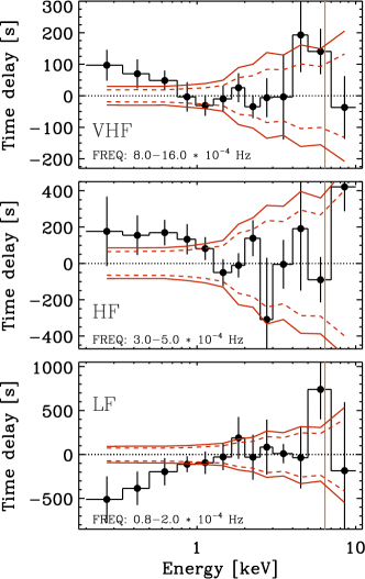
Figure 3: Lag-energy spectrum for low (LF; $0.8-2.0\times 10^{-4}$ Hz), high (HF; $3-6\times 10^{-4}$ Hz) and very high (VHF; $8-14\times 10^{-4}$ Hz) frequencies. A 1.2–4.0 keV reference band was used. The red dashed and solid lines are the 90 and 95 per cent confidence intervals respectively, on the assumption of zero ‘true’ lag.

Figure 4: Lag-energy spectrum for low frequencies (LF; $0.8-2.0\times 10^{-4}$ Hz) using a 0.3–10.0 keV reference band. The plot shows a continual increase in lag from low to high energies, and are consistent with the lower panel in Fig. 3 where a 1.2–4.0 keV reference band is used.

Motivated by the lag-frequency plot, we calculate the lag-energy over three frequency ranges, one focused on the hard lags ($0.8-2\times 10^{-4}$ Hz, low frequency, hereafter LF), one centred around the most negative (soft) lags ($3-5\times 10^{-4}$ Hz, high frequency, hereafter HF), and one spanning the remaining negative (soft) lags ($8-16\times 10^{-4}$ Hz, very high frequency, hereafter VHF).

Figure 3 shows the lag as a function of energy for the LF, HF and VHF frequencies. At LF (lower panel) the soft energies lead the 1.2-4.0 keV reference band, with the delay increasing with energy separation. This is consistent with results found in BH-XRBs (e.g Miyamoto & Kitamoto 1989; Nowak et al. 1999) and AGN (e.g. Arévalo et al. 2008; Zoghbi et al. 2011; Kara et al. 2013). A possible ($2\sigma$ significance) lag in the iron K band can be seen, which lags behind the 1.2–4.0 keV reference band by $\sim 500-1000$ s. In Fig.4 we show the LF lag-energy spectrum computed using the broad 0.3-10 keV energy band. A continual increase in the lag with energy is seen, and is consistent with the LF lag-energy plot of Fig. 3.

At HF (middle panel), the softer energies lag the reference band, in agreement with the lag-frequency spectrum in Fig 2. The lag below $\sim 1$ keV is $\sim 200$ s behind the reference band. No iron K$\alpha$ lag can be seen in the data.

At VHF (upper panel in Fig. 3) the soft energies (below $\sim 0.6$ keV) lag the reference band by up to 100 s. Also evident is a feature around iron K$\alpha$ with a lag of $\sim 150$ s.

The difference in lag-energy between the two soft lag frequency ranges (HF and VHF) is surprising. This is the first time that the soft lags have been examined as a function of frequency, and the differences indicate that different processes may be dominating at these two different timescales. We assess the significance of this result firstly by assessing the significance of the lags in the VHF as this regime is more susceptible to Poisson noise, particularly at high energies. We use $10^{4}$ Monte Carlo simulations of well-correlated light curves with zero ‘true lag’, with the properties (power spectra, count rates) of the real data. The 90 and 95 per cent confidence intervals are shown as the red dashed and solid lines in Fig. 3. The low energy continuum (below 0.6 keV) and iron line lags are both detected at $\sim 2\sigma$ significance. We also show the 90 and 95 percent confidence intervals for the HF and LF in Fig. 3. The soft lag is detected at $>2\sigma$ confidence at energies below 1 keV in the HF. At LF, the soft lead at energies below $\sim 0.8$ keV is detected at $>2\sigma$, as well as the lag in the iron K$\alpha$ band.

4.2 Modelling the lag-energy spectra

                 .

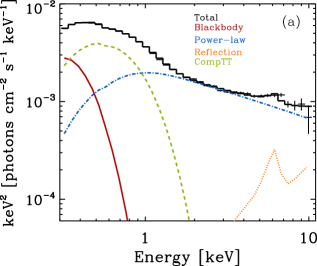
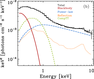
Figure 5: a) Left: neutral reflection model: blackbody (red solid), an absorbed power-law emission (blue dot-dashed), separate soft excess component (green dashed), and neutral reflection (orange dotted). b) Right: ionised reflection model including a blackbody (red solid), absorbed power-law emission (blue dot-dashed), a separate soft excess component (green dashed), and ionised reflection (orange dotted). The data are the ‘unfolded’ time-averaged EPIC-pn spectra (see J13).

                 .

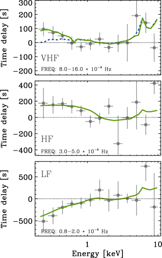
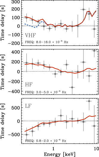
Figure 6: a) Left: simulated lag-energy spectra for the neutral reflection model, at low (LF; $0.8-2.0\times 10^{-4}$ Hz), high (HF; $3-6\times 10^{-4}$ Hz) and very high (VHF; $8-14\times 10^{-4}$ Hz) frequencies. A 1.2–4.0 keV reference band was used. The green line represents the model including the black body, whereas the blue dashed line does not include a lag from this component. b) Right: simulated lag-energy spectrum for the ionised reflection model, for the LF, HF and VHF ranges. The red line represents the models including the black body, whereas the blue dashed line does not include a lag from this component.

J13 presented several spectral models to explain the time averaged spectrum and the covariance spectra. In this section we re-examine these models in terms of their lag-energy predictions. We model the resulting lag-energy spectra using simulations, similar to the method of Kara et al. (2013). We simulated identical sets of light curves for each energy bin, including independent Poisson noise in each. The light curves of each component (at each energy) were time-shifted and then combined weighted by the strength of the component in the mean spectrum at a given energy. The lag-energy spectra at each frequency were modelled independently, with each component having a different magnitude at each frequency. This is clearly a simplification of the effects of an impulse response function on each spectral component, but allows us to approximate the shape of the lag-energy spectrum resulting from the combined effects of multiple components.

4.2.1 Neutral reflection and a separate soft excess

We first use the spectral components identified in J13 (see Fig. 5a), where there is a blackbody from intrinsic disc emission (red), a separate soft excess component (green) which provides seed photons to produce the coronal emission from Compton upscattering (blue). This coronal emission illuminates the disc and produces a (mostly) neutral reflection spectrum (black) from a region with inner radius of $\sim 15R_{g}$. The soft excess component is modelled with comptt (Titarchuk & Lyubarskij 1995, representing incomplete thermalisation of the inner accretion disc (see Done et al. 2012).

For slow variability, where we are seeing propagation time delays, we assume that the blackbody disc emission leads, followed by the soft excess, followed by the corona. This gives a good match to the LF lag-energy spectra if the soft excess lags 400 seconds behind the blackbody, and the corona lags by 1500 seconds behind the blackbody. A reflection lag of 2 ks behind the corona is included, to model any reflection that is occurring on top of the propagation delays at LF. The soft band emission then leads the hard band by $\sim 1000$ seconds, as required by the lag-frequency fits (see Fig. 2). These simulated LF lag-energy spectra are shown in the lower panel of Fig. 6.

The HF lag energy can be matched by assuming that some part of the soft excess emission is reprocessed on short timescales, so that it lags behind the corona by 300 seconds (middle panel in Fig. 6). No iron K$\alpha$ is seen in the data at this frequency, but we include a 300 second lag for this feature. If an iron K$\alpha$ reflection feature is observed at VHF, and at LF with a longer delay than in the VHF, then we might also expect to see this feature at HF. Its presence in the LF suggests this feature has not been smeared out over the timescale of interest, and hence why we expect to observe it at HF.

An iron line is instead seen in the VHF lag-energy plot. This can be well described if some fraction of the reflected emission lags 200 seconds behind the fastest coronal variability. However, this cannot reproduce the low energy lag seen in the VHF (blue simulations in upper panel of Fig. 6). This is better fit by the shape of the blackbody disc. The green simulations in the upper panel of Fig. 6 show the VHF lag-energy prediction if both the blackbody and reflected emission lag 200 seconds behind the fastest coronal variability.

4.2.2 Ionized reflection and a separate soft excess

The model above is an extreme interpretation of the spectrum. The reflector is likely to be ionized to some extent, so we explore how this might change the reverberation predictions. We allow reflection to be ionised in the fits. We describe this using the rfxconv model (Kolehmainen et al. 2011), which is a convolution version of the Ross & Fabian (2005) ionized reflection models, but also include an additional soft excess as is required by the fast covariance spectra (J13). However, this gives a best fitting model ($\chi^{2}$ = 2204 / 1799 d.o.f) to the time averaged EPIC spectrum for fairly low ionisation $\log\xi=1.3$, which is again not highly smeared by relativistic effects ($R_{\rm in}=10R_{\rm g}$ for standard emissivity of $\eta(r)\propto r^{-3}$). This does not produce much more low energy reflection than the original models, so instead we fix $\log\xi=3$ to explore the impact of the maximal contribution of reflection at low energies. This gives a slightly worse fit with $\chi^{2}$ = 2220 / 1800 d.o.f, and requires $R_{\rm in}=3R_{\rm g}$ in order to smooth the low energy atomic features, and so implies high spin, in contrast to the intrinsic disc component in this source which implies low spin (Done et al. 2013). This spectral model is shown in Fig. 5b.

The lag prediction from this maximal reflection model are shown in Fig. 6b, calculated using the same lags for each component as before. They are not dramatically different to those from neutral reflection, possibly because the ionised reflection is still a small fraction of the soft band flux, relative to the other components. The additional blackbody variability is still required in the VHF to match the soft lag seen in these data as the reflected emission follows the illuminating spectrum, and there is a downturn in the illuminating spectrum at low energies due to the seed photon energy for Compton upscattering being within the observed bandpass (J13). This downturn limits the amount of reflection at the lowest energies.

5 Discussion and Conclusions

We show that the X-ray time delays as a function of energy and Fourier-frequency can be constrained in the ‘simple’ NLS1 PG 1244+026 using a 120 ks XMM-Newton observation. The lag as a function of frequency between a hard (1.2–4.0 keV) and a soft (0.3-1 keV) energy band shows the now well established switch from a hard lag at low frequencies to a soft lag at high frequencies. The maximum soft lag of $\sim 200$ s is at $\sim 4\times 10^{-4}$ Hz but there is also evidence for a second negative lag of $\sim 100$ s at $\sim 1.2\times 10^{-3}$ Hz.

Modelling the lag-frequency spectrum with simple response functions gives an acceptable fit if both hard and soft bands contain both direct emission (modelled using a $\delta$-function response) and a smoothed, time-delayed response (approximated by a top hat response function). We interpret the lagged response in two different ways in the two different bands, with the hard band lag being a result of propagation time delays while the soft band lag results from reprocessing of the primary X-ray spectrum. The soft band response function has a maximum time delay of $\sim 1500$ s. For a black hole mass of $\sim 10^{7}\hbox{$M_{\mathrm{BH}}$}$, this corresponds to reprocessing within $\sim 20R_{\rm g}$ of the illuminating source.

We consider the lag as a function of energy in three frequency ranges. The lag-energy data are consistent with the interpretation above. The lowest frequency lag-energy spectra shows the long timescale variability has a lag which increases systematically with energy (Fig. 3). This is expected from propagating fluctuations through the accretion flow, where the disc, soft excess and harder X-ray emission from a spatially extended corona are produced at progressively smaller radii. The slow variability originates in the disc, propagates to the soft excess, then propagates to the corona. Each component has its own lag, but the smoothly varying change in the contribution of each component with energy results in a smooth lag-energy spectrum. We also find evidence for a disc reflection component responding on this timescale.

On shorter timescales, we would not expect the propagating fluctuations to correlate at all across the spectrum, as the disc and soft excess probably cannot vary much intrinsically on these timescales. The soft lag at these frequencies is therefore interpreted as reprocessing of the intrinsic power-law emission. We split the frequency band over which the soft lag is seen into two, and find evidence for a change in the lag-energy spectra with frequency. The high frequency (HF) variability appears to show a stronger reprocessing response in the soft excess rather than in the reflected component; there is no significant lag at iron K$\alpha$ seen in the data, but only at energies below 1.2 keV. The VHF has a lag at iron (and redward) energies, but this is accompanied not by the soft excess but by the blackbody.

The hard X-ray emission from the corona is consistent with an origin in inverse-Compton scattering. The downturn below 0.8 keV in the covariance indicates that the source of seed photons is the soft excess (J13). This strongly limits the amount of reflection which can contribute to the spectrum below 1 keV. Thus reflection alone is not the only source of lags in this object. An obvious additional source is thermal reprocessing - the thermalisation of the non-reflected, absorbed emission, which leads to heating of the disc and soft excess regions as they respond to increased illumination. This could give a physical explanation as to why these components are seen to reverberate along with the reflection component. However, it is strange that the soft excess emission requires typically longer to respond to the coronal illumination than the blackbody and iron line. The propagation lags clearly show that the soft excess region lags the blackbody, and under the assumption that these are modulated by the same inwardly propagating fluctuations, is smaller and closer in than the blackbody. We would expect its reprocessed signature to be more evident at higher frequencies than the blackbody as it is closer to the coronal emission region. It may be that the region producing the soft excess has little reflected or reprocessed flux (perhaps because it is too highly ionised), but that it responds to the corona via propagation lags on the blackbody disc response.

The hard band PSD (Fig. 1) shows weaker variability power than the soft band at frequencies below $\sim 2\times 10^{-4}$ Hz (LF). At frequencies above $\sim 2\times 10^{-4}$ Hz (HF) the power in each band is comparable, with the hard showing a slight excess in power. The hard band shows an obvious excess in power exactly where the VHF soft lag occurs. The coherence also drops to $\sim 0.5$ just above the HF band. This drop in coherence is most easily explained as due to the ‘cross over’ between two independently varying components with quite different energy spectra. At LF and VHF bands, where one component dominates the PSD in both bands, the coherence is high since each component is correlated with itself.

Clearly the timing and variability properties of this simple spectrum source are very interesting. Better estimates of the lag-energy and lag-frequency properties, only possible with much longer observations, are needed to fully understand the causal connection between the emission components in this highly promising source.

Additional note

After the original submission of this manuscript we learnt that the X-ray time lags in PG 1244+026 were simultaneously and independently studied by Kara et al. (2013). That submitted paper focuses on the iron K$\alpha$ reverberation lags at low frequencies, whereas this paper has focused on understanding the soft lags, and the time lags observed up to higher frequencies. The data analysis in the two papers are consistent, with the differences in the lag energy spectra presented in each paper resulting from the choice of reference band. These two papers highlight the need to better constrain the variability and time delays up to higher frequencies in this source.

References

- Alston et al. (2013) Alston W. N., Vaughan S., Uttley P., 2013, MNRAS, 435, 1511
- Arévalo et al. (2008) Arévalo P., McHardy I. M., Summons D. P., 2008, MNRAS, 388, 211
- Arévalo et al. (2006) Arévalo P., Papadakis I. E., Uttley P., McHardy I. M., Brinkmann W., 2006, MNRAS, 372, 401
- Arévalo & Uttley (2006) Arévalo P., Uttley P., 2006, MNRAS, 367, 801
- Ballet (1999) Ballet J., 1999, A&AS, 135, 371
- Bendat & Piersol (1986) Bendat J., Piersol A., 1986, Random data: analysis and measurement procedures. A Wiley-Interscience publication, Wiley
- Boller et al. (1996) Boller T., Brandt W. N., Fink H., 1996, A&A, 305, 53
- Cackett et al. (2013) Cackett E. M., Fabian A. C., Zogbhi A., Kara E., Reynolds C., Uttley P., 2013, ApJL, 764, L9
- Campana & Stella (1995) Campana S., Stella L., 1995, MNRAS, 272, 585
- Crummy et al. (2006) Crummy J., Fabian A. C., Gallo L., Ross R. R., 2006, MNRAS, 365, 1067
- Davis (2001) Davis J. E., 2001, ApJ, 562, 575
- De Marco et al. (2013) De Marco B., Ponti G., Cappi M., Dadina M., Uttley P., Cackett E. M., Fabian A. C., Miniutti G., 2013, MNRAS, 431, 2441
- Done et al. (2012) Done C., Davis S. W., Jin C., Blaes O., Ward M., 2012, MNRAS, 420, 1848
- Done et al. (2013) Done C., Jin C., Middleton M., Ward M., 2013, MNRAS, 434, 1955
- Emmanoulopoulos et al. (2011) Emmanoulopoulos D., McHardy I. M., Papadakis I. E., 2011, MNRAS, 416, L94
- Fabian et al. (2004) Fabian A. C., Miniutti G., Gallo L., Boller T., Tanaka Y., Vaughan S., Ross R. R., 2004, MNRAS, 353, 1071
- Fabian et al. (2009) Fabian A. C., Zoghbi A., Ross R. R., Uttley P., Gallo L. C., Brandt W. N., Blustin A. J., Boller T., Caballero-Garcia M. D., Larsson J., Miller J. M., Miniutti G., Ponti G., Reis R. C., Reynolds C. S., Tanaka Y., Young A. J., 2009, Nature, 459, 540
- Gallo (2006) Gallo L. C., 2006, MNRAS, 368, 479
- Gierliński & Done (2004) Gierliński M., Done C., 2004, MNRAS, 349, L7
- Jin et al. (2013) Jin C., Done C., Middleton M., Ward M., 2013, MNRAS, 436, 3173
- Jin et al. (2012a) Jin C., Ward M., Done C., 2012a, MNRAS, 422, 3268
- Jin et al. (2012b) Jin C., Ward M., Done C., 2012b, MNRAS, 425, 907
- Kara et al. (2013) Kara E., Cackett E. M., Fabian A. C., Reynolds C., Uttley P., 2013, ArXiv e-prints
- Kara et al. (2013) Kara E., Fabian A. C., Cackett E. M., Miniutti G., Uttley P., 2013, MNRAS, 430, 1408
- Kara et al. (2013) Kara E., Fabian A. C., Cackett E. M., Steiner J. F., Uttley P., Wilkins D. R., Zoghbi A., 2013, MNRAS, 428, 2795
- Kolehmainen et al. (2011) Kolehmainen M., Done C., Díaz Trigo M., 2011, MNRAS, 416, 311
- Kotov et al. (2001) Kotov O., Churazov E., Gilfanov M., 2001, MNRAS, 327, 799
- McHardy et al. (2007) McHardy I. M., Arévalo P., Uttley P., Papadakis I. E., Summons D. P., Brinkmann W., Page M. J., 2007, MNRAS, 382, 985
- McHardy et al. (2004) McHardy I. M., Papadakis I. E., Uttley P., Page M. J., Mason K. O., 2004, MNRAS, 348, 783
- Middleton et al. (2007) Middleton M., Done C., Gierliński M., 2007, MNRAS, 381, 1426
- Miller et al. (2010) Miller L., Turner T. J., Reeves J. N., Lobban A., Kraemer S. B., Crenshaw D. M., 2010, MNRAS, 403, 196
- Miyamoto & Kitamoto (1989) Miyamoto S., Kitamoto S., 1989, Nature, 342, 773
- Miyamoto et al. (1988) Miyamoto S., Kitamoto S., Mitsuda K., Dotani T., 1988, Nature, 336, 450
- Nowak et al. (1999) Nowak M. A., Vaughan B. A., Wilms J., Dove J. B., Begelman M. C., 1999, ApJ, 510, 874
- Nowak et al. (1999) Nowak M. A., Wilms J., Vaughan B. A., Dove J. B., Begelman M. C., 1999, ApJ, 515, 726
- Papadakis et al. (2001) Papadakis I. E., Nandra K., Kazanas D., 2001, ApJL, 554, L133
- Pottschmidt et al. (2000) Pottschmidt K., Wilms J., Nowak M. A., Heindl W. A., Smith D. M., Staubert R., 2000, A&A, 357, L17
- Revnivtsev et al. (1999) Revnivtsev M., Gilfanov M., Churazov E., 1999, A&A, 347, L23
- Reynolds (1999) Reynolds C. S., 1999, in Poutanen J., Svensson R., eds, High Energy Processes in Accreting Black Holes Vol. 161 of Astronomical Society of the Pacific Conference Series, Compton Reflection and Iron Fluorescence in Active Galactic Nuclei and Galactic Black Hole Candidates. p. 178
- Reynolds (2000) Reynolds C. S., 2000, ApJ, 533, 811
- Ross & Fabian (2005) Ross R. R., Fabian A. C., 2005, MNRAS, 358, 211
- Stella (1990) Stella L., 1990, Nature, 344, 747
- Strüder et al. (2001) Strüder L., Briel U., Dennerl K., Hartmann R., 2001, A&A, 365, L18
- Titarchuk & Lyubarskij (1995) Titarchuk L., Lyubarskij Y., 1995, ApJ, 450, 876
- Uttley et al. (2011) Uttley P., Wilkinson T., Cassatella P., Wilms J., Pottschmidt K., Hanke M., Böck M., 2011, MNRAS, 414, L60
- Vaughan & Nowak (1997) Vaughan B. A., Nowak M. A., 1997, ApJL, 474, L43
- Vaughan et al. (2002) Vaughan S., Boller T., Fabian A. C., Ballantyne D. R., Brandt W. N., Trümper J., 2002, MNRAS, 337, 247
- Vaughan et al. (2003) Vaughan S., Edelson R., Warwick R. S., Uttley P., 2003, MNRAS, 345, 1271
- Vaughan et al. (2003) Vaughan S., Fabian A. C., Nandra K., 2003, MNRAS, 339, 1237
- Walton et al. (2013) Walton D. J., Nardini E., Fabian A. C., Gallo L. C., Reis R. C., 2013, MNRAS, 428, 2901
- Wilkins & Fabian (2013a) Wilkins D. R., Fabian A. C., 2013a, MNRAS, 430, 247
- Wilkins & Fabian (2013b) Wilkins D. R., Fabian A. C., 2013b, MNRAS, 430, 247
- Zoghbi & Fabian (2011) Zoghbi A., Fabian A. C., 2011, MNRAS, 418, 2642
- Zoghbi et al. (2011) Zoghbi A., Uttley P., Fabian A. C., 2011, MNRAS, 412, 59