On Conformal Divergences and their Population Minimizers^‡

Abstract

Total Bregman divergences are a recent tweak of ordinary Bregman divergences originally motivated by applications that required invariance by rotations. They have displayed superior results compared to ordinary Bregman divergences on several clustering, computer vision, medical imaging and machine learning tasks. These preliminary results raise two important problems : First, report a complete characterization of the left and right population minimizers for this class of total Bregman divergences. Second, characterize a principled superset of total and ordinary Bregman divergences with good clustering properties, from which one could tailor the choice of a divergence to a particular application. In this paper, we provide and study one such superset with interesting geometric features, that we call conformal divergences, and focus on their left and right population minimizers. Our results are obtained in a recently coined $(u,v)$-geometric structure that is a generalization of the dually flat affine connections in information geometry. We characterize both analytically and geometrically the population minimizers. We prove that conformal divergences (resp. total Bregman divergences) are essentially exhaustive for their left (resp. right) population minimizers. We further report new results and extend previous results on the robustness to outliers of the left and right population minimizers, and discuss the role of the $(u,v)$-geometric structure in clustering. Additional results are also given.

1 Introduction

Loosely defined in its most general form, the clustering problem is related to the grouping of a data sample according to unknown classes or clusters [1]. One of the most popular and well-posed approaches to clustering is centroid-based: it seeks to summarize data into a fixed set of cluster centers — or population minimizers — that best describe the sample, where ”best” is understood with respect to an expected measure of distortion to the whole sample [2, 3]. Because of their convexity properties and links to likelihoods in exponential families, ordinary Bregman divergences are often used to compute these distortions in clustering algorithms, such as in $k$-means and EM [4, 2, 3]. Their left and right population minimizers are respectively a cluster’s $f$-mean [5, 6] and the cluster’s average (ordinary Bregman divergences are in general not symmetric). It has been shown that modulo technical assumptions, ordinary Bregman divergences are exhaustive for their right population minimizer: any divergence whose population minimizer is the sample average is a Bregman divergence [7, 8]. This shows that the scope of $k$-means and EM is wide and encompasses all domains whose “natural” distortion measures rely on Bregman divergences, such as signal processing, Euclidean geometry, information theory, statistics, etc. .

There has been a recent burst of interest in a new class of divergences, built from Bregman divergences, known as total Bregman divergences [9, 10, 11, 12, 13, 14, 15, 16, 17, 18]. These divergences are invariant to particular transformations of the natural space. Experimentally speaking, clustering with their left population minimizers yields significantly improved results compared to ordinary Bregman divergences in domains like DTI interpolation and segmentation [9]. These results exploit the fact that the left population minimizers of total Bregman divergences are weighted generalized $f$-means [9]. In the general context of clustering, and also for reasons related to statistics and maximum likelihood estimation [19], it is important to characterize further the population minimizers of total Bregman divergences: important questions include the characterization of their right population minimizers and the exhaustivity of these divergences for their population minimizers. In the context of clustering, the results of [9] also contribute to the advocacy that clustering is in fact a domain dependent method [1], thereby raising the question of how we may generalize further the set of candidate (total or ordinary) Bregman divergences, while keeping good properties, from which one may select the best candidates to solve a particular problem.

In this paper, we address these questions in a setting which generalizes in two ways total and ordinary Bregman divergences. First, we consider a superset of total Bregman divergences and ordinary Bregman divergences that we define as conformal divergences. Second, we consider a coordinate system which is not the usual dually flat affine coordinate system of (total, ordinary) Bregman divergences, but a generalization in information geometry studied by Zhang and Amari, defined as the $(u,v)$-geometric structure [20, 21, 22], in which two coordinate mappings $u$ and $v$ define the gradient (and its reciprocal inverse) of the generator of the Bregman divergence.

In this generalized setting, our main contribution includes:

• the characterization of the right population minimizers for total Bregman divergences;

• the characterization of the right population minimizer for an interesting $L_{p}$ generalization of total Bregman divergences;

• a proof that conformal divergences are exhaustive for their left population minimizers;

• a proof that total Bregman divergences are exhaustive for their right population minimizers;

• the robustness analysis of the left and right population minimizers for conformal divergences, which generalizes results known for total Bregman divergences [9].

Our contribution also includes results pertinent for clustering, such as (i) a proof that the $(u,v)$-geometric structure sometimes describe an equivalence relation which might be useful in the context of clustering; (ii) a proof that the square loss in $v$-coordinates is the only 1D symmetric conformal divergence in the $(u,v)$-geometric structure; (iii) a discussion on population minimizers for a further extension involving the recently coined scaled Bregman divergences (that generalize Csiszár’s $f$-divergences) [19].

The paper is structured as follows. The following Section gives definitions. Section 3 compares the various notions of divergences we consider. Section 4 is devoted to left population minimizers of conformal divergences in the $(u,v)$-geometric structure. Section 5 does the same for right population minimizers. Section 6 studies the robustness of the population minimizers and Section 7 discusses our results. A last section concludes. In order not to laden the paper’s body, some proofs are given in an Appendix in Section 10. The rest of the proofs, not in the published version, appear from page 10.8 in this extended version.

2 Definitions

Throughout this paper, bold faces denote column vectors, such as $\bm{0}$ for the null vector, while capitals, like $J$ or $\mathrm{H}$ (respectively Jacobian and Hessian) denote matrices. Coordinates are noted in exponent, such as $x^{1},x^{2},...,x^{d}$ for vector $\bm{x}\in{\mathbb{R}}^{d}$, where $d\geq 1$.

A (right-sided) conformal divergence, $D_{\varphi,g}$, is parameterized by two real-valued functions $\varphi$ and $g$ with $\mathrm{im}g\subseteq(0,+\infty)$, whose domains are a compact convex of ${\mathbb{R}}^{d}$. The expression of $D_{\varphi,g}$ is:

$$D_{\varphi,g}(\bm{x}:\bm{y}) \stackrel{{\scriptstyle\mathrm{.}}}{{=}} g(\bm{y})D_{\varphi}(\bm{x}:\bm{y})\>\>.$$ (1)

$\varphi$ is real-valued strictly convex twice differentiable, and $D_{\varphi}(\bm{x}:\bm{y})$ is the ordinary Bregman divergence with generator $\varphi$:

$$D_{\varphi}(\bm{x}:\bm{y}) = \varphi(\bm{x})-\varphi(\bm{y})-(\bm{x}-\bm{y})^{\top}\nabla\varphi(\bm{y})\>\>.$$ (2)

$\nabla\varphi$ denotes the gradient of $\varphi$. $g$ admits continuous directional derivatives: function $\mathrm{D}_{{\bm{z}}}g(\bm{x})\stackrel{{\scriptstyle\mathrm{.}}}{{=}}\lim_{t\rightarrow 0}\mathrm{D}_{t,{\bm{z}}}g(\bm{x})$, defining directional derivatives, is continuous and exist for any valid direction $\bm{z}$ such that $\mathrm{D}_{t,\bm{z}}g(\bm{x})$ is defined in a neighborhood of 0 (with respect to $t$). We give:

$$\mathrm{D}_{t,\bm{z}}g(\bm{x}) \stackrel{{\scriptstyle\mathrm{.}}}{{=}} \frac{g(\bm{x}+t\bm{z})-g(\bm{x})}{t}\>\>.$$

Ordinary Bregman divergences match the subset of conformal divergences for which $g(.)=K$, a constant. The most popular recent example of conformal divergences is obtained for $g=Kg_{\bot}$ for some constant $K>0$ and :

$$g_{\bot}(\bm{y}) \stackrel{{\scriptstyle\mathrm{.}}}{{=}} \frac{1}{\sqrt{1+\|\nabla\varphi(\bm{y})\|_{2}^{2}}}\>\>,$$ (3)

which defines total Bregman divergences, that are invariant to rotations of the coordinate axes [10, 12, 13, 17, 14, 15, 16] (among others). Table II presents some examples of total Bregman divergences (with $K=1$). Remark that $g_{\bot}(\bm{y})$ is of the form $f_{\bot}(\nabla\varphi(\bm{y}))$, with

$$f_{\bot}(\bm{x}) \stackrel{{\scriptstyle\mathrm{.}}}{{=}} \frac{1}{\sqrt{1+\|\bm{x}\|_{2}^{2}}}\>\>.$$ (4)

Figure 1 depicts $D_{\varphi}(x:y)$ and $D_{\varphi,g_{\bot}}(x:y)$ on a simple example.

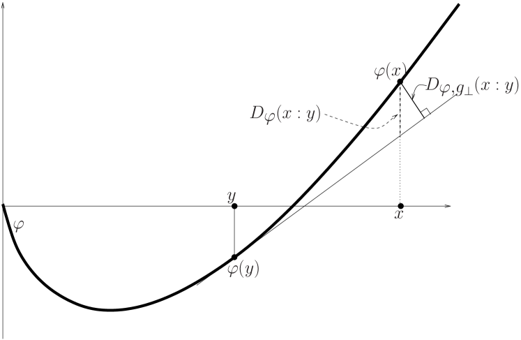
Figure 1: Depiction of $D_{\varphi}(x:y)$ and $D_{\varphi,g_{\bot}}(x:y)$ when $\varphi(x)=x\ln(x)-x$.

We also investigate the generalization of (3) to $p$-norms, and define, $\forall p\geq 1$:

$$g_{p}(\bm{y}) \stackrel{{\scriptstyle\mathrm{.}}}{{=}} f_{p}(\nabla\varphi(\bm{y}))\>\>;$$ (5)

$$f_{p}(\bm{x}) \stackrel{{\scriptstyle\mathrm{.}}}{{=}} \frac{1}{\left(1+\|\bm{x}\|_{p}^{p}\right)^{\frac{1}{p}}}\>\>.$$ (6)

The $p$-norm of $\bm{x}$ is $\|\bm{x}\|_{p}\stackrel{{\scriptstyle\mathrm{.}}}{{=}}\left(\sum_{i}|x^{i}|^{p}\right)^{\frac{1}{p}}$.

A coordinate mapping $v$ is a $C^{1}$, bijective function $v:{\mathbb{R}}^{d}\rightarrow{\mathbb{R}}^{d}$. For any coordinate mapping $v$, we define the $v$-conformal divergence $D^{v}_{\varphi,g}$ as:

$$D^{v}_{\varphi,g}(\bm{x}:\bm{y}) \stackrel{{\scriptstyle\mathrm{.}}}{{=}} g(\bm{y})D_{\varphi}(v(\bm{x}):v(\bm{y}))\>\>.$$ (7)

$v$-conformal divergences are inspired by divergences in the $(u,v)$ geometric structure [20, 21] (see also Section 7). They generalize conformal divergences for which $v=\mathrm{Id}$. We shall investigate several interesting cases of $v$-conformal divergences, including those where $g$ is a function of $\nabla\varphi$, and those where $g$ is a function of coordinate mapping $u$ in the $(u,v)$-geometric structure.

Let us now motivate the $(u,v)$-geometric structure in the context of the dual coordinate systems of ordinary Bregman divergences [23]. Function $g$ in $v$-conformal divergences depends on the right parameter of the divergence. We shall see (Lemma 7) that when $g$ is not constant, the $v$-conformal divergence cannot be symmetric: $g(\bm{y})D_{\varphi}(v(\bm{x}):v(\bm{y}))\neq g(\bm{y})D_{\varphi}(v(\bm{y}):v(\bm{x}))$. However, our results extend at little cost to left-sided conformal divergences, i.e. whose regularization factor $g$ depends on the left parameter of the divergence. Indeed, calling to convex conjugates, we obtain:

$$D_{\varphi,g}^{v}(\bm{x}:\bm{y})$$

$$= g(\bm{y})D_{\varphi}(v(\bm{x}):v(\bm{y}))$$

$$= g(\bm{y})D_{\varphi^{\star}}((\nabla\varphi\circ v)(\bm{y}):(\nabla\varphi\circ v)(\bm{x}))$$

$$= g(\bm{y})D_{\varphi^{\star}}(u(\bm{y}):u(\bm{x}))\>\>,$$

where $u\stackrel{{\scriptstyle\mathrm{.}}}{{=}}\nabla\varphi\circ v$ also defines a coordinate mapping and $\varphi^{\star}$ is the convex conjugate of $\varphi$. Any such coordinate mappings $u$ and $v$ such that $u\circ v^{-1}$ defines the gradient of a strictly convex differentiable function $\varphi$ is called an $(u,v)$-geometric structure [20], that we write $(u,v)_{\varphi}$ from now on, to make explicit the reference to $\varphi$.

We now define population minimizers for conformal divergences.

Definition 1

(left- and right-population minimizers) Let ${\mathcal{S}}\stackrel{{\scriptstyle\mathrm{.}}}{{=}}\{\bm{x}_{1},\bm{x}_{2},...,\bm{x}_{n}\}$, with $\bm{x}_{i}\in{\mathbb{R}}^{d},\forall i=1,2,...,n$. Let $D:{\mathbb{R}}^{d}\times{\mathbb{R}}^{d}\rightarrow{\mathbb{R}}$ be the shorthand for some ordinary Bregman (resp. conformal, resp. $v$-conformal) divergence $D_{\varphi}$ (resp. $D_{\varphi,g}$, resp. $D_{\varphi,g}^{v}$). A left population minimizer for $D$ on ${\mathcal{S}}$ is any $\bm{\mu}$ such that $\sum_{i}{D(\bm{\mu}:\bm{x}_{i})}=\min_{\bm{x}}\sum_{i}D(\bm{x}:\bm{x}_{i})$. A right population minimizer for $D$ on ${\mathcal{S}}$ is any $\bm{\mu}$ such that $\sum_{i}{D(\bm{x}_{i}:\bm{\mu})}=\min_{\bm{x}}\sum_{i}D(\bm{x}_{i}:\bm{x})$.

This definition, as well as the results in this paper, can be extended to non uniform distributions over ${\mathcal{S}}$, and to population minimizers in the continuous case.

3 On divergences: ordinary, total and conformal

There is a need to generalize the source of divergences from which efficient centroid-based clustering algorithms may be derived. The comparison between ordinary Bregman and total Bregman divergences is enlightening from that standpoint: ordinary Bregman divergences $D_{\varphi}$ are axiomatically characterized as the unique family of divergences (under mild conditions) that yield their right population minimizers matching the sample average [8]. Hence, the right population minimizer is the simplest to compute, but having fixed the data sample, regardless of the generator of the divergence $\varphi$, it is always the same. From a clustering standpoint, it may be more intuitive that since changing the generator changes the geometry of the problem, it should possibly change this population minimizer as well. Also, this invariance is not convenient to further optimize the population minimizer by tuning the divergence at hand.

This problem does not appear anymore with total Bregman divergences. Initially, total Bregman divergences [9] $D_{\varphi,g_{\bot}}$ have been geometrically designed to enforce invariance by rotations in the parameter space [9], thus mimicking the ordinary/total least squares relationships. Rotation invariance is a very desirable property in medical imaging [16] and computer vision [18]. Thus, total Bregman divergences have been specifically engineered to solve a particular geometric problem, which has led to improved results on several key applications related to clustering. Besides, total Bregman divergences have also proven experimentally superior in boosting [13] and tensor-based graph matching [11], etc., just to name a few. One theoretical argument that explains the superiority of total Bregman divergences was detailed in [17], where it was proved that total Bregman divergences are robust compared to ordinary Bregman divergences, by studying the impact of outliers via the influence function.

The difference between total and ordinary Bregman divergences can also be captured from a statistical standpoint. It is well-known that regular exponential families $p(\bm{x};\bm{\theta})=h(\bm{x})\exp(\bm{\theta}^{\top}\bm{t}(\bm{x})-\varphi(\bm{\theta}))$ are in bijection with (regular) Bregman divergences [4], $p(\bm{x};\bm{\theta})=h(\bm{x})\exp(-D_{\varphi^{\star}}(\bm{t}(\bm{x}):\bm{\eta}(\bm{\theta})))$ where $\bm{\eta}(\bm{\theta})=\nabla\varphi(\bm{\theta})$ is the dual moment parameter, and that the Maximum Likelihood Estimator (MLE) for $n$ identically and independently distributed observations of an exponential family coincides with the so-called observed point in information geometry [23]: $\overline{\bm{t}}=(1/n)\sum_{i}\bm{t}(\bm{x}_{i})$, where $\bm{t}(.)$ denotes the vector of sufficient statistics of the exponential families under consideration. That is, the MLE $\hat{\bm{\eta}}$ expressed in the $\bm{\eta}$-parameter matches the centroid of sufficient statistics: $\hat{\bm{\eta}}=\overline{\bm{t}}$. Since there is also a bijection between ordinary and total Bregman divergences, we deduce by transitivity with the ordinary Bregman-exponential family bijection that we can associate an exponential family $p(\bm{x};\bm{\theta})=h(\bm{x})\exp(-D_{\varphi^{\star},g_{\bot}}(\bm{t}(\bm{x}):\bm{\eta})\sqrt{1+\|\nabla\varphi^{\star}(\bm{\eta})\|^{2}})$ to any total Bregman divergence $D_{\varphi^{\star},g_{\bot}}$. This statistical distribution $p(\bm{x};\bm{\theta})$ corresponds also to a lifted exponential family $\tilde{p}(\tilde{\bm{x}};\tilde{\bm{\theta}})$ in disguise, as exemplified in [17] with $\tilde{\bm{\theta}}=(\bm{\theta},\varphi(\bm{\theta}))$ and $\tilde{\bm{x}}=(1/\sqrt{1+\|\nabla\varphi(\bm{x})\|^{2}})\cdot(\bm{x},1)$. In other words, the ordinary exponential family is lifted to the space having one extra dimension and embedded as a hypersurface. Now, it can be proved that the total (left) observed point is the Bayesian MAP estimator in the lifted exponential family with prior distribution $\pi(\bm{\theta})=\exp(-n\tilde{\varphi}(\bm{\theta}))$, where $\tilde{\varphi}(\bm{\theta})$ is the normalization factor. Table I compares properties of ordinary and total Bregman divergences. ”Information” relates to the sample divergence to the right population minimizer [4].

	ordinary Bregman divergence	total Bregman divergence
Right population minimizer	centroid	this paper (Corollary 1)
Left population minimizer	$\nabla\varphi$-mean, weights $w_{i}=1/n$	$\nabla\varphi$-mean, weights $w_{i}=1/\sqrt{1+\|\nabla\varphi(\bm{x}_{i})\|^{2}}$
Robustness of pop. minimizers	no	yes
Information	Bregman information	this paper (Lemma 3)
Exhaustiveness	right pop. minimizer = sample average	this paper (Theorem 2)
Bijection	exponential families	lifted exponential families
Inference	MLE = observed point	Bayesian MAP = total observed point
	($\hat{\bm{\eta}}$=right population minimizer)	(left population minimizer)

TABLE I: Properties of ordinary Bregman vs total Bregman divergences.

Our definition of conformal divergences is inspired by information geometry. In information geometry [23], a divergence [22, 24] (also called a contrast function or yoke) is a measure of dissimilarity $D(\bm{p}:\bm{q})$ (with $D(\bm{p}:\bm{q})\geq 0$ with equality iff $p=q$, but not necessarily symmetric nor satisfying the triangle inequality) that further needs to satisfy some smoothness conditions [22] to induce properly a metric tensor and a cubic form (for the coefficients of the connections). In Riemannian geometry, a conformal metric $\textsl{g}^{\prime}$ of a metric g is expressed by $\textsl{g}^{\prime}=\varrho\textsl{g}$, where $\varrho>0$ (hence also written as $\textsl{g}^{\prime}=e^{\varrho}\textsl{g}$). The uniformization theorem states that Riemannian surfaces are conformally equivalent to either the spherical, planar or hyperbolic manifolds — all of constant curvatures. In our definition of conformal divergences in eq. (7), factor $g(.)$ plays the role of the conformal factor; we shall see in Lemma 3 below that it indeed defines a conformal factor. In the particular case of total Bregman divergences, $\varrho\propto 1/\sqrt{1+\|\nabla\varphi(.)\|^{2}}$ plays the role of the conformal factor. In information geometry induced by a generalized logarithm function, a conformal flattening [25] allows to obtain a dually flat structure. Conformal mappings also explain the role of escort distributions, and yield efficient algorithms for Voronoi diagrams induced by conformal divergences, a geometric structure particularly relevant to clustering [25, 26].

4 Left population minimizers of $v$-conformal divergences

We are interested in this Section in characterizing the left population minimizers of general $v$-conformal divergences. We build on results known from [17, 14] for the elicitation of the left population minimizer when $v=\mathrm{Id}$, and the well known results from [8] for the elicitation of the divergences having the arithmetic average as right population minimizer. Technicalities are simpler than for the right population minimizers because function $g$ does not depend on the left parameter of $D_{\varphi}$. We first show that the left population minimizer of some $v$-conformal divergence $D_{\varphi,g}^{v}$ is a weighted $u$-mean, where $(u,v)_{\varphi}$ is a geometric structure.

Lemma 1

The left population minimizer $\bm{\mu}$ of any $v$-conformal divergence $D_{\varphi,g}^{v}$ on ${\mathcal{S}}$ is unique and equals:

$$\bm{\mu} = u^{-1}\left(\frac{1}{\sum_{i}g(\bm{x}_{i})}\sum_{i}g(\bm{x}_{i})u(\bm{x}_{i})\right)\>\>,$$ (8)

where $(u,v)_{\varphi}$ is a geometric structure.

(Proof in Appendix, Subsection 10.1) We now show that the characterization of left population minimizers for $v$-conformal divergences is exhaustive, as any distortion function admitting a weighted $u$-mean as left population minimizer equals a $v$-conformal divergence $D_{\varphi,g}^{v}$, for some $(u,v)_{\varphi}$-geometric structure.

Lemma 2

Let $\mu\stackrel{{\scriptstyle\mathrm{.}}}{{=}}u^{-1}(\sum_{i}{w_{i}u(\bm{x}_{i})})$ be the unique solution to $\min_{\bm{x}}\sum_{i}{D(\bm{x}:\bm{x}_{i})}$, where:

1. $D:{\mathbb{R}}^{d}\times{\mathbb{R}}^{d}\rightarrow{\mathbb{R}}$ is non-negative, twice continuously differentiable and such that $D(\bm{x}:\bm{x})=0,\forall\bm{x}$;

2. $u:{\mathbb{R}}^{d}\rightarrow{\mathbb{R}}^{d}$ is a coordinate mapping;

3. $\sum_{i}w_{i}=1$ and $w_{i}>0,\forall i$.

Then there exist a function $g:{\mathbb{R}}^{d}\rightarrow{\mathbb{R}}$ admitting continuous directional derivatives and a geometric structure $(u,v)_{\varphi}$ such that

$$D(\bm{x}:\bm{y}) = D^{v}_{\varphi,g}(\bm{x}:\bm{y})\>\>.$$ (9)

(Proof in Appendix, Subsection 10.2)

5 Right population minimizers of $v$-conformal divergences

5.1 Case $v=\mathrm{Id}$

We now derive the right population minimizers for a conformal divergence $D_{\varphi,g}$, thus considering $v$-conformal divergences with $v=\mathrm{Id}$. Because $g$ admits continuous directional derivatives, so does $D_{\varphi,g}(\bm{x}:\bm{y})$ for both its arguments. Let us define:

$$\mathrm{D}_{t,\bm{z}}D_{\varphi,g}(\bm{x}:\bm{y})$$ (10)

$$\stackrel{{\scriptstyle\mathrm{.}}}{{=}} \frac{D_{\varphi,g}(\bm{x}:\bm{y}+t\bm{z})-D_{\varphi,g}(\bm{x}:\bm{y})}{t}\>\>,$$

so that the directional derivative in the right parameter $\mathrm{D}_{\bm{z}}D_{\varphi,g}(\bm{x}:\bm{y})\stackrel{{\scriptstyle\mathrm{.}}}{{=}}\lim_{t\rightarrow 0}\mathrm{D}_{t,\bm{z}}D_{\varphi,g}(\bm{x}:\bm{y})$ exists, for any valid direction $\bm{z}$. Define from any ${\mathcal{S}}$ the following averages:

$$\overline{\varphi} \stackrel{{\scriptstyle\mathrm{.}}}{{=}} \frac{1}{n}\sum_{i}\varphi(\bm{x}_{i})\>\>,$$ (11)

$$\overline{\bm{x}} \stackrel{{\scriptstyle\mathrm{.}}}{{=}} \frac{1}{n}\sum_{i}\bm{x}_{i}\>\>.$$ (12)

Let us define the following vectors $\overline{\bm{x}}^{+},\bm{\mu}^{+},\bm{\delta}^{+},\bm{z}^{+}\in{\mathbb{R}}^{d+1}$:

$$\overline{\bm{x}}^{+} \stackrel{{\scriptstyle\mathrm{.}}}{{=}} \left[\begin{array}[]{c}\overline{\bm{x}}\\ \overline{\varphi}\end{array}\right]\>\>,$$ (15)

$$\bm{\mu}^{+} \stackrel{{\scriptstyle\mathrm{.}}}{{=}} \left[\begin{array}[]{c}\bm{\mu}\\ \varphi(\bm{\mu})\end{array}\right]\>\>,$$ (18)

$$\bm{\delta}^{+} \stackrel{{\scriptstyle\mathrm{.}}}{{=}} \overline{\bm{x}}^{+}-\bm{\mu}^{+}\>\>,$$ (19)

$$\bm{z}^{+} \stackrel{{\scriptstyle\mathrm{.}}}{{=}} \left[\begin{array}[]{c}\mathrm{D}_{\bm{z}}(g(\bm{\mu})\nabla\varphi(\bm{\mu}))\\ -\mathrm{D}_{\bm{z}}g(\bm{\mu})\end{array}\right]\>\>,$$ (22)

from which we define the following sets:

$${\mathbb{P}}_{{\mathcal{S}},\varphi,g} \stackrel{{\scriptstyle\mathrm{.}}}{{=}} \left\{\bm{\mu}\in\mathrm{dom}(D_{\varphi,g}):\bm{\delta}^{+}\bot\bm{z}^{+},\forall\bm{z}\right\}\>\>,$$ (23)

where the directions $\bm{z}$ have to be valid, i.e. such that the directional derivative of $g$ is defined in a neighborhood of 0 (with respect to $t$). We also define ${\mathbb{B}}_{\varphi,g}$, the eventually empty set of non-differentiable boundary points of the intersection of the domains of $\varphi$ and $g$. In the following, we let $\mathcal{P}(D_{\varphi,g};{\mathcal{S}})$ denote the set of right population minimizers for conformal divergence $D_{\varphi,g}$ on set ${\mathcal{S}}$.

Lemma 3

$\mathcal{P}(D_{\varphi,g};{\mathcal{S}})\subseteq{\mathbb{P}}_{{\mathcal{S}},\varphi,g}\cup{\mathbb{B}}_{\varphi,g}$. Furthermore, $\forall\bm{\mu}\in{\mathbb{P}}_{{\mathcal{S}},\varphi,g}\backslash\{\overline{\bm{x}}\}$, the average distortion is a weighted square Mahalanobis distance to the population average:

$$\frac{1}{n}\sum_{i}D_{\varphi,g}(\bm{x}_{i}:\bm{\mu})$$ (24)

$$= \varrho_{g}\times(\overline{\bm{x}}-\bm{\mu})^{\top}\mathrm{H}\varphi(\bm{\mu})(\overline{\bm{x}}-\bm{\mu})\>\>,$$

with $\varrho_{g}\stackrel{{\scriptstyle\mathrm{.}}}{{=}}g^{2}(\bm{\mu})/\mathrm{D}_{(\overline{\bm{x}}-\bm{\mu})}g(\bm{\mu})>0$.

(Proof in Appendix, Subsection 10.3) With respect to the discussion on conformal divergences in Section 3, we see that $\varrho_{g}$ defines a conformal factor, and so all points in ${\mathbb{P}}_{{\mathcal{S}},\varphi,g}\backslash\{\overline{\bm{x}}\}$ are points for which the conformal divergence reduces to a (square) distance on metric $\mathrm{H}\varphi$ conformally transformed. We shall see that set ${\mathbb{P}}_{{\mathcal{S}},\varphi,g}\backslash\{\overline{\bm{x}}\}$ also contains population minimizers. Finally, Lemma 3 shows that the conformal Bregman information generalizes the Bregman information [4] to weighted square Mahalanobis distance — because Bregman divergences can be formulated as square Mahalanobis distance over particular metrics, Bregman information can also be expressed using square Mahalanobis distance.

We are now ready to state a first Theorem that provides the right population minimizers for a subset of conformal divergences which encompasses total Bregman divergences.

Theorem 1

Pick $g=Kg_{p}$ as in (5) with $K>0$ a constant, $p=2k/(2k-1)$ and $k\in{\mathbb{N}}_{*}$. Then, assuming ${\mathbb{B}}_{\varphi,g}=\emptyset$, the right population minimizer(s) for $D_{\varphi,g_{p}}$ on ${\mathcal{S}}$ match the set:

$$\mathcal{P}(D_{\varphi,Kg_{p}};{\mathcal{S}}) = \arg\min_{\bm{\mu}}\|\overline{\bm{x}}^{+}-\bm{\mu}^{+}\|_{q}\>\>,$$ (25)

with $\overline{\bm{x}}^{+}$ and $\bm{\mu}^{+}$ defined in (15) and (18), and $q=2k\in{\mathbb{N}}$ is the Hölder conjugate of $p$.

(Proof in Appendix, Subsection 10.4)

Fixing $k=1$ allows to retrieve the right population minimizers for total Bregman divergences. Because of their importance, we state their characterization as a separate corollary.

Corollary 1

Consider $g=Kg_{\bot}$ for some constant $K>0$. The following holds true:

$$\bm{\delta}^{+} \bot \left[\begin{array}[]{c}\nabla\varphi(\bm{\mu})\\ \|\nabla\varphi(\bm{\mu})\|_{2}^{2}\end{array}\right]\>\>,\forall\bm{\mu}\in{\mathbb{P}}_{{\mathcal{S}},\varphi,g_{\bot}}\>\>;$$ (28)

i.e., the orthogonal projection of $(\overline{\bm{x}},\overline{\varphi})$ on the tangent hyperplane $T_{\varphi}(\bm{\mu})$ to $\varphi$ at $\bm{\mu}$ is point $(\bm{\mu},\varphi(\bm{\mu}))$. Furthermore, assuming ${\mathbb{B}}_{\varphi,g}=\emptyset$, we have:

$$\mathcal{P}(D_{\varphi,Kg_{\bot}};{\mathcal{S}}) = \arg\min_{\bm{\mu}}\|\overline{\bm{x}}^{+}-\bm{\mu}^{+}\|_{2}\>\>,$$ (29)

with $\overline{\bm{x}}^{+}$ and $\bm{\mu}^{+}$ defined in (15) and (18).

Figure 2 (left) displays how to find $\bm{\mu}$ which meets condition (28). Notice that, by construction, the right population minimizer for $D_{\varphi,Kg_{\bot}}$ is invariant by rotation of the axes. Figure 2 (right) depicts the construction of the population minimizer in a simple 1D case.

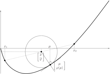
Figure 2: Left: how to find $\bm{\mu}$ as stated in Corollary 1: the orthogonal projection of point $(\overline{\bm{x}},\overline{\varphi})$ on the hyperplane $T_{\varphi}(\bm{\mu})$ tangent to $\varphi$ at $\bm{\mu}$ coincides with point $(\bm{\mu},\varphi(\bm{\mu}))$. The blue region depicts the subset of the epigraph of $\varphi$ which is below the image by $\varphi$ of the convex envelope of ${\mathcal{S}}$. Right: computation of the (unique) population minimizer on a simple 1D example with $\varphi(x)=x\ln x-x$, following Corollary 1. Remark that $\mu>\overline{x}$ in this case.

We now study to what extent total Bregman divergences are exhaustive for the construction of the right population minimizer depicted in Corollary 1. It has been shown that ordinary Bregman divergences are exhaustive for the expectation as right population minimizer, i.e. if the expectation is the right population minimum of a loss $D(x:y)$, then under mild conditions this loss is an ordinary Bregman divergence [7, 8]. It turns out that total Bregman divergence are also exhaustive for their right population minimizer. For the sake of simplicity, we are going to show the result in the one-dimensional setting ($d=1$). For this objective, we let:

$${\mathbb{P}}_{{\mathcal{S}},\varphi}$$ (34)

$$\stackrel{{\scriptstyle\mathrm{.}}}{{=}} \left\{\mu\in{\mathbb{R}}:\left[\begin{array}[]{c}\overline{x}-\mu\\ \overline{\varphi}-\varphi(\mu)\end{array}\right]\bot\left[\begin{array}[]{c}1\\ \varphi^{\prime}(\mu)\end{array}\right]\right\}\>\>.$$

When $\mu\neq\overline{x}$, the condition is equivalent to

$$\tilde{\varphi}^{\prime}_{\mathcal{S}}(\mu)\varphi^{\prime}(\mu) = -1\>\>,$$ (35)

with

$$\tilde{\varphi}^{\prime}_{\mathcal{S}}(z) \stackrel{{\scriptstyle\mathrm{.}}}{{=}} \frac{\overline{\varphi}-\varphi(z)}{\overline{x}-z}\>\>,\forall z\in\mathrm{dom}(\varphi)\backslash\{\overline{x}\}\>\>,$$ (36)

Theorem 2

Let $D:{\mathbb{R}}\times{\mathbb{R}}\rightarrow{\mathbb{R}}$ be a function differentiable such that $D(x:y)$ is twice continuously differentiable in $x$, and satisfies the following assumptions: (i) $D(x:x)=0,\forall x$, (ii) $D(x:y)>0,\forall y\neq x$, (iii) $D$ is invariant by rotation of the axes, (iv) the right population minimizer of $D$ on ${\mathcal{S}}=\{x_{1},x_{2},...,x_{n}\}$ is unique and satisfies $\{\mu\}\in{\mathbb{P}}_{{\mathcal{S}},\varphi}$ for some strictly convex twice differentiable $\varphi$. Then

$$D(x:y) = D_{\varphi,Kg_{\bot}}(x:y)\>\>,$$ (37)

where $K>0$ is a constant and $g_{\bot}$ is defined in eq. (3).

(proof in Subsection 10.8)

5.2 Case $v$ arbitrary

We now focus on general $v$-conformal divergences with $(u,v)_{\varphi}$ a geometric structure. In order not to laden this Section and its notations, we make the simplifying assumption that ${\mathbb{B}}_{\varphi,g}=\emptyset$. This is not restrictive: even in the multidimensional extension of the total Bregman divergences of Table II, the cardinal of ${\mathbb{B}}_{\varphi,g}=\emptyset$ would be at most one, so the main structural and algorithmic issues to characterize the right population minimizers essentially lie in the characterization of ${\mathbb{P}}_{{\mathcal{S}},\varphi}$. Define from ${\mathcal{S}}$ the following averages:

$$\overline{\varphi}_{v} \stackrel{{\scriptstyle\mathrm{.}}}{{=}} \frac{1}{n}\sum_{i}\varphi(v(\bm{x}_{i}))$$

$$= \frac{1}{n}\sum_{i}u(\bm{x}_{i})^{\top}v(\bm{x}_{i})-\overline{\varphi^{\star}}_{u}\>\>;$$

$$\overline{\bm{x}}_{v} \stackrel{{\scriptstyle\mathrm{.}}}{{=}} \frac{1}{n}\sum_{i}v(\bm{x}_{i})\>\>.$$ (39)

We first state a generalization of Theorem 1 to arbitrary $(u,v)_{\varphi}$-geometric structures.

Theorem 3

Let $(u,v)_{\varphi}$ be a geometric structure. Pick $g=Kg_{p}^{u}(\bm{\mu})$ with $g_{p}^{u}(\bm{\mu})\stackrel{{\scriptstyle\mathrm{.}}}{{=}}f_{p}(u(\bm{\mu}))$, $f_{p}$ is defined in (6), $K>0$ is a constant, and $p=2k/(2k-1)$ with $k\in{\mathbb{N}}_{*}$. Then, the right population minimizer(s) for the $v$-conformal divergence $D^{v}_{\varphi,Kg^{u}_{p}}$ on ${\mathcal{S}}$ match the set:

$$\mathcal{P}(D^{v}_{\varphi,Kg^{u}_{p}};{\mathcal{S}}) = \arg\min_{\bm{\mu}}\|\overline{\bm{x}}^{+}_{v}-\bm{\mu}^{+}_{v}\|_{q}\>\>,$$ (40)

with $\overline{\bm{x}}^{+}_{v}$ and $\bm{\mu}^{+}_{v}$ defined in (51) and (56), and $q=2k\in{\mathbb{N}}$ is the Hölder conjugate of $p$.

(Proof omitted) We also provide the following generalization of Corollary 1, which stands as a Corollary to Theorem 3.

Corollary 2

Let $(u,v)_{\varphi}$ be a geometric structure. Pick $g(\bm{\mu})=Kg^{u}_{\bot}(\bm{\mu})\stackrel{{\scriptstyle\mathrm{.}}}{{=}}Kf_{\bot}(u(\bm{\mu}))$ for any constant $K>0$. Any right population minimizer $\bm{\mu}$ for the $v$-conformal divergence $D^{v}_{\varphi,Kg^{u}_{\bot}}$ satisfies:

$$\left[\begin{array}[]{c}\overline{\bm{x}}_{v}-v(\bm{\mu})\\ \overline{\varphi}_{v}-\varphi(v(\bm{\mu}))\end{array}\right] \bot \left[\begin{array}[]{c}u(\bm{\mu})\\ \|u(\bm{\mu})\|_{2}^{2}\end{array}\right]\>\>.$$ (45)

Furthermore, we have:

$$\mathcal{P}(D^{v}_{\varphi,Kg^{u}_{\bot}};{\mathcal{S}}) = \arg\min_{\bm{\mu}}\|\overline{\bm{x}}_{v}^{+}-\bm{\mu}_{v}^{+}\|_{2}\>\>,$$ (46)

with $\overline{\bm{x}}^{+}_{v}$ and $\bm{\mu}^{+}_{v}$ defined as follows:

$$\overline{\bm{x}}^{+}_{v} \stackrel{{\scriptstyle\mathrm{.}}}{{=}} \left[\begin{array}[]{c}\overline{\bm{x}}_{v}\\ \overline{\varphi}_{v}\end{array}\right]=\left[\begin{array}[]{c}\overline{\bm{x}}_{v}\\ \frac{1}{n}\sum_{i}u(\bm{x}_{i})^{\top}v(\bm{x}_{i})-\overline{\varphi^{\star}}_{u}\end{array}\right]\>\>,$$ (51)

$$\bm{\mu}^{+}_{v} \stackrel{{\scriptstyle\mathrm{.}}}{{=}} \left[\begin{array}[]{c}v(\bm{\mu})\\ \varphi(v(\bm{\mu}))\end{array}\right]=\left[\begin{array}[]{c}v(\bm{\mu})\\ u(\bm{\mu})^{\top}v(\bm{\mu})-\varphi^{\star}(u(\bm{\mu}))\end{array}\right]\>\>.$$ (56)

(Proof omitted) Finally, we provide a general characterization of the population minimizers for a general $g=f\circ u$. This is a generalization of the orthogonality property in (45), which is interesting since $\bm{\delta}^{+}$ is formulated in the $v$ coordinate mapping while $\bm{z}^{+}$ is formulated in the $u$ coordinate mapping.

Theorem 4

Let $(u,v)_{\varphi}$ be a geometric structure. Suppose $g(\bm{x})=f(u(\bm{x}))$, with $f$ differentiable. For any ${\mathcal{S}}$ and any $\bm{\mu},\bm{z}\in{\mathbb{R}}^{d}$, define $\bm{\delta}^{+}_{v},\bm{z}^{+}_{u}\in{\mathbb{R}}^{d+1}$ with:

$$\bm{\delta}^{+}_{v} \stackrel{{\scriptstyle\mathrm{.}}}{{=}} \left[\begin{array}[]{c}\overline{\bm{x}}_{v}-v(\bm{\mu})\\ \overline{\varphi}_{v}-\varphi(v(\bm{\mu}))\end{array}\right]=\underbrace{\left[\begin{array}[]{c}\overline{\bm{x}}_{v}\\ \overline{\varphi}_{v}\end{array}\right]}_{\bm{x}^{+}_{v}}-\underbrace{\left[\begin{array}[]{c}v(\bm{\mu})\\ \varphi(v(\bm{\mu}))\end{array}\right]}_{\bm{\mu}^{+}_{v}}\>\>,$$ (63)

$$\bm{z}^{+}_{u} \stackrel{{\scriptstyle\mathrm{.}}}{{=}} \left[\begin{array}[]{c}f(u(\bm{\mu}))\times\bm{z}+\nabla f(u(\bm{\mu}))^{\top}\bm{z}\times u(\bm{\mu})\\ -\nabla f(u(\bm{\mu}))^{\top}\bm{z}\end{array}\right]\>\>.$$ (66)

Then any right population minimizer $\bm{\mu}$ for the $v$-conformal divergence $D^{v}_{\varphi,g}$ satisfies $\bm{\delta}^{+}_{v}\bot\bm{z}^{+}_{u}$, for any valid direction $\bm{z}$.

(Proof omitted)

6 Robustness of the population minimizers

Suppose we add an outlier element $\bm{x}_{*}$ with small weight $0<\epsilon<1$ to $\mathcal{S}$. The population minimizer (left or right) of $\mathcal{S}$, $\bm{\mu}$, eventually drifts to a new population minimizer $\bm{\mu}_{*}=\bm{\mu}+\epsilon\bm{\delta}_{\bm{\mu}}$ of ${\mathcal{S}}\cup\{\bm{x}_{*}\}$. $\bm{\delta}_{\bm{\mu}}$ is called the influence function of $\bm{x}_{*}$ [9]. A population minimizer is robust to outliers iff the magnitude of $\bm{\delta}_{\bm{\mu}}$ is bounded, as explained in the following definition where $0<\tau<1$ is any small constant.

Definition 2

The population minimizer of some divergence $D$ is robust to outliers when, for any outlier $\bm{x}_{*}$ and any weight $0<\epsilon<1-\tau$, $\|\bm{\delta}_{\bm{\mu}}\|_{2}\leq C$, where $C$ does not depend upon $\bm{x}_{*}$ nor $\epsilon$.

Robustness according to Definition 2 is stronger than in the model of [9, 16] as our robustness strictly implies theirs (which relies on very small weights $\epsilon$). So the Lemma to follow is a twofolds generalization of the results of [9, 16], not only from the standpoint of the divergences, but also from the model’s.

Lemma 4

Let $(u,v)_{\varphi}$ be a geometric structure. Suppose the following assumptions are verified: (i) $g(\bm{x})=O(1),\forall\bm{x}$, (ii) $\|u(\bm{x})\|_{2}=O(1/g(\bm{x})),\forall{\bm{x}}$, (iii) the minimal eigenvalue of $J_{u}^{\top}J_{u}$ is $\lambda>0$, $J_{u}$ being the Jacobian of $u$. Then under assumptions (i-iii), the left population minimizer of $v$-conformal divergence $D^{v}_{\varphi,g}$ is robust to outliers.

(proof in Subsection 11) Lemma 4 generalizes the robustness of the left population centers of total Bregman divergences (Theorem III.2 in [16]), for which $g=Kg_{\bot},v=\mathrm{Id},u=\nabla\varphi$ (the Jacobian of $u$ being the Hessian of $\varphi$, it satisfies assumption (iii) since $\varphi$ is strictly convex).

The right population minimizer is unfortunately not robust to outliers for any $g$ according to Definition 2, yet it satisfies in a general setting of $v$-conformal divergences, a weaker notion of robustness which says that the influence function must be properly bounded by a divergence between $\bm{x}_{*}$ and $\bm{\mu}$, as long as $\bm{x}_{*}$ does not deviate too much from $\bm{\mu}$ in the $v$-coordinate mapping. This last notion exploits the fact that convex function are locally Lipschitz.

Definition 3

Let $(u,v)_{\varphi}$ be a geometric structure. The population minimizer of some $v$-conformal divergence $D^{v}_{\varphi,g}$ is $K$-weakly robust to outliers when for any outlier $\bm{x}_{*}$ and any weight $0<\epsilon<1$:

$$|\varphi(v(\bm{x}_{*}))-\varphi(v(\bm{\mu}))|\leq L\|v(\bm{x}_{*})-v(\bm{\mu})\|_{2}$$ (67)

$$\Rightarrow\|\bm{\delta}_{\bm{\mu}}\|_{2}\leq K\ell(L)\|\bm{x}_{*}-\bm{\mu}\|_{2}\>\>,$$

where $K\geq 0$ is not a function of $\bm{x}_{*}$ or $\epsilon$, and $\ell(L)$ is a linear function in $L$.

We now show that the right population minimizer is $K$-weakly robust to outliers, for a $K$ which depends solely on the coordinate mapping $v$. We assume in the Lemma that $\bm{0}\in\mathrm{im}u$, which is a mild assumption as it postulates in the $(u,v)_{\varphi}$-geometric structure that the gradient $\nabla_{\varphi}$ has a root in coordinate mapping $v$. We exploit the fact that any matrix $A\in{\mathbb{R}}^{d\times d}$ satisfies $A^{\top}A\succeq 0$, where “$\succeq$” means positive semi-definite.

Lemma 5

Let $(u,v)_{\varphi}$ be a geometric structure, and let $f\stackrel{{\scriptstyle\mathrm{.}}}{{=}}g\circ u^{-1}$. We make the following assumptions: (i) $\bm{0}\in\mathrm{im}u$, (ii) $f(\bm{z})\neq 0,\forall\bm{z}$, (iii) the ratio of the maximal to the minimal eigenvalue of $J_{v}^{\top}J_{v}$, noted $\lambda_{v}$, is finite, where $J_{v}$ is the Jacobian of $v$. Then the right population minimizer of $v$-conformal divergence $D^{v}_{\varphi,g}$ is $\sqrt{\lambda_{v}}$-weakly robust to outliers.

(Proof in Subsection 12)

7 Discussion

In this Section, we discuss several aspects of population minimizers in the setting of conformal divergences; in particular, we discuss further the geometric structure relation, the approximation of the right population minimizers in the 1D setting, the existence of symmetric conformal divergences, and the uniqueness of the right population minimizer.

The nature of the $(u,v)_{\varphi}$-geometric structure relation — The $(u,v)_{\varphi}$-geometric structure has been introduced in the context of information geometry to provide a way to compute and analyze the dually flat $(\bm{\eta},\bm{\theta})$ coordinate system arising e.g. in exponential families and ordinary Bregman divergences, through a single source parameter which is originally a distribution [20]. To state the key result about the $(u,v)_{\varphi}$-geometric structure, we consider two strictly monotonous differentiable functions $u(\xi)$ and $v(\xi)$ with $u(0)=v(0)=0$. Consider the positive measures on $\mathbb{R}^{d+1}_{+}$, and denote by $m(x,\xi)=\sum_{i=1}^{d+1}\xi_{i}{{1\!\!1}}_{x=x_{i}}$ a positive distribution computed from $\mathcal{S}=\{x_{1},x_{2},...,x_{d+1}\}$, where ${1\!\!1}$ is the indicator variable. $\bm{\xi}\stackrel{{\scriptstyle\mathrm{.}}}{{=}}[\xi_{1}\>\>\xi_{2}\>\>...\>\>\xi_{d+1}]^{\top}$ defines a coordinate system from which we may define two coordinate systems $\bm{\eta},\bm{\theta}$ of ${\mathbb{R}}^{d+1}$ with $\theta^{i}\stackrel{{\scriptstyle\mathrm{.}}}{{=}}u(\xi_{i})$ and $\eta^{i}\stackrel{{\scriptstyle\mathrm{.}}}{{=}}v(\xi_{i})$. These coordinate systems have the following interesting information-geometric properties.

Theorem 5

[20] The $(u,v)_{\varphi}$-geometric structure is dually flat, with the following two potential functions:

$$\psi(\bm{\theta}) \stackrel{{\scriptstyle\mathrm{.}}}{{=}} \sum\int\int\frac{v^{\prime}(u^{-1}(\theta^{i}))}{u^{\prime}(u^{-1}(\theta^{i}))}(\mathrm{d}\theta^{i})^{2}\>\>,$$

$$\varphi(\bm{\eta}) \stackrel{{\scriptstyle\mathrm{.}}}{{=}} \sum\int\int\frac{u^{\prime}(v^{-1}(\eta^{i}))}{v^{\prime}(v^{-1}(\eta^{i}))}(\mathrm{d}\eta^{i})^{2}\>\>;$$

the divergence between two $\bm{p}$ and $\bm{q}$ is given by:

$$D(\bm{p};\bm{q}) \stackrel{{\scriptstyle\mathrm{.}}}{{=}} \psi(\bm{\theta}_{\bm{p}})+\varphi(\bm{\eta}_{\bm{q}})-\bm{\theta}_{\bm{p}}\cdot\bm{\eta}_{\bm{q}}\>\>,$$

and the metric in the $\bm{\theta}$ coordinate system is:

$$g_{ij}(\bm{\theta}) \stackrel{{\scriptstyle\mathrm{.}}}{{=}} \frac{v^{\prime}(\xi_{i})}{u^{\prime}(\xi_{i})}\delta_{ij}\>\>.$$

One may check that $u\circ v^{-1}$ defines $\nabla\varphi$, and that $D$ is an ordinary Bregman divergence. One important example is Amari’s $(\alpha,\beta)$ structure ($\alpha,\beta>0$) for which $u(\xi_{i})\stackrel{{\scriptstyle\mathrm{.}}}{{=}}\xi_{i}^{\alpha}$ and $v(\xi_{i})\stackrel{{\scriptstyle\mathrm{.}}}{{=}}\xi_{i}^{\beta}$, which helps to see the usefulness of the $(u,v)_{\varphi}$-geometric structure in the context of clustering: assuming $\bm{\xi}$ is a source parameter recorded in data, one can jointly tune $\alpha,\beta$ to tune the coordinate system of the divergence without changing its generator $\varphi$ as long as $\alpha/\beta$ remains a fixed constant (because $\varphi(\bm{\eta})=(1+\alpha/\beta)^{-1}\sum_{i}\eta_{i}^{1+\alpha/\beta}$, omitting the additive constant which does not change the divergence). Thus, we get new free parameters to tune that adapt the coordinate system from which the divergence is computed, which we may use to get improved clustering results.

We now show that, if we accept to change the generator, then we may have a significant freedom in picking and changing the coordinate mappings $u$ and $v$. We study the nature of the $(u,v)_{\varphi}$-geometric structure, and define a tolerance relation [27] as a binary relation which is reflexive and symmetric but not necessarily transitive. An equivalence relation is reflexive, symmetric and transitive. We consider the “geometric structure” binary relation, $(u,v)$ (without reference to $\varphi$), which holds when there exists some $\varphi$ such that $(u,v)_{\varphi}$ is a geometric structure.

Lemma 6

The “geometric structure” relation is a tolerance relation. It is an equivalence relation in the subset of functions ${\mathcal{S}}_{\phi}$ indexed by some strictly convex differentiable $\phi$ and defined by: ${\mathcal{S}}_{\phi}\stackrel{{\scriptstyle\mathrm{.}}}{{=}}\{\varphi:\mathrm{H}\varphi(\nabla\phi)=\mathrm{H}\phi P_{\phi}D_{\phi}^{-1}DP_{\phi}^{\top}\}$, where $P_{\phi},D_{\phi}$ are the eigenspace and eigenvalues matrix of $\mathrm{H}\phi$ and $D\succ 0$ is diagonal.

(Proof in Appendix, Subsection 10.5) Hence, for example, the geometric structure relation is an equivalence relation on any subset of positive definite quadratic forms that have the same eigenspace. The compactness and convexity of some of these subgroups ${\mathcal{S}}_{\phi}$ may be interesting from the clustering standpoint to learn the $(u,v)_{\varphi}$-geometric structure (see Section 5).

Simple right population minimizers — The following corollary is a safe-check of Lemma 3 which states when the right population minimizer has simple forms.

Corollary 3

Suppose ${\mathcal{S}}$ contains at least two distinct elements. The right population minimizer of $D_{\varphi,g}$ on set ${\mathcal{S}}$ is:

1. always the arithmetic average (i.e. $\bm{\mu}=\overline{\bm{x}}$) iff $g(\bm{y})$ is constant;

2. always the $\varphi$-mean (i.e. $\varphi(\bm{\mu})=\overline{\varphi}$) iff $\varphi(\bm{x})=K\int 1/h(\bm{u}^{\top}\bm{x})+K^{\prime}$, with (i) $K,K^{\prime}$ and vector $\bm{u}$ constants, (ii) $g(\bm{x})=h(\bm{u}^{\top}\bm{x})$ for some function $h:{\mathbb{R}}\rightarrow{\mathbb{R}}$ strictly monotonous with derivative sign opposite to that of $K$.

(proof in Subsection 13)

Only one symmetric conformal divergence — We show that there exists a single 1D symmetric conformal divergence in the $(u,v)_{\varphi}$-geometric structure, the square loss, $D_{\varphi,g}(v(x):v(y))\propto(v(x)-v(y))^{2}$. As a corollary, it shows that there is no symmetric total Bregman divergence. The proof is made in the 1D case, that is, when the domain and image of $u$ and $v$ is ${\mathbb{R}}$, and it can be extended at no cost to $d$D separable conformal divergences, for which $g(u(\bm{y}))D_{\varphi}(v(\bm{x}):v(\bm{y}))\stackrel{{\scriptstyle\mathrm{.}}}{{=}}\sum_{i}g(u(y^{i}))D_{\varphi}(v(x^{i}):v(y^{i}))$.

Lemma 7

Let $(u,v)_{\varphi}$ be a geometric structure and $D_{\varphi,g}$ a conformal divergence for some strictly convex twice differentiable $\varphi$. Suppose that $\forall x,y$:

$$g(u(y))D_{\varphi}(v(x):v(y))$$ (68)

$$= g(u(x))D_{\varphi}(v(y):v(x))\>\>.$$

Then (i) $g(.)=K_{1}$, (ii) $v=\ell(u)$, (iii) $\varphi(x)=K_{2}x^{2}+\ell(x)$ for some constants $K_{1}>0,K_{2}>0$, where $\ell(.)$ is a linear function in its argument.

(proof in Subsection 14) Thus, conformal divergence are not metrics, yet they can be used to craft metrics. To ensure that symmetry and triangle inequality are met without violating non-negativity nor the identity of indiscernibles, we can search for the $\alpha\in(0,1]$ with which $(g(u(\bm{y}))D_{\varphi}(v(\bm{x}):v(\bm{y}))+g(u(\bm{x}))D_{\varphi}(v(\bm{y}):v(\bm{x})))^{\alpha}$ meets the triangle inequality, or use [28]’s method.

Fast approximation of right population minimizers — We now show that under mild assumptions on $\varphi$, candidates for right population minimizer may be easily located and approximated in the 1D setting. Assume wlog that ${\mathcal{S}}$ is ordered, that is $x_{1}\leq x_{2}\leq...\leq x_{n}$. Whenever $\varphi$ is bijective over $[x_{1},x_{n}]$, we define the $\varphi$-mean:

$$\overline{x}_{\varphi} \stackrel{{\scriptstyle\mathrm{.}}}{{=}} \varphi^{-1}(\overline{\varphi})\>\>.$$

Let us denote a candidate right population minimizer as a real which is solution of (35). Candidate population minimizers are critical points for the right parameter of the average divergence [29].

Lemma 8

Suppose $g(y)=Kg_{\bot}(y)$, and assume that $\varphi^{\prime}$ has constant sign on $[x_{1},x_{n}]$. Then there exists a candidate right population minimizer $\mu$ in $[x_{1},x_{n}]$. Furthermore, $\mu\in[\overline{x}_{\varphi},\overline{x}]$ if $\mathrm{sign}=-$, and $\mu\in[\overline{x},\overline{x}_{\varphi}]$ if $\mathrm{sign}=+$. Here, “$\mathrm{sign}$” denotes the sign of $\varphi^{\prime}$ over $[x_{1},x_{n}]$.

(Proof in Appendix, Subsection 10.6)

$\varphi(x)$	Name or expression	$\overline{x}_{\varphi}$	Name of	Location
	for $D_{\varphi,g_{\bot}}(x:y)$		$\varphi$-mean
$-\log(x)$	Total Itakura-Saito	$\prod_{i}{x_{i}^{\frac{1}{n}}}$	Geometric mean	$[\overline{x}_{\varphi},\overline{x}]$
$1/x$	$\frac{1}{x}-\frac{2}{y}+\frac{x}{y^{2}}$	$n/\sum_{i}{x^{-1}_{i}}$	Harmonic mean	$[\overline{x}_{\varphi},\overline{x}]$
$x^{2}$	Total square loss	$\pm\sqrt{\frac{1}{n}\sum_{i}{x^{2}_{i}}}$	$\pm$ Root mean square	$[\overline{x},\overline{x}_{\varphi}]$ or $[\overline{x}_{\varphi},\overline{x}]$
$x^{p},p\geq 2$	Total power loss	$\left(\sum_{i}{x^{p}_{i}}\right)^{\frac{1}{p}}$	Power mean	$[\overline{x},\overline{x}_{\varphi}]$
$\exp(x)$	Total exp divergence	$\log\sum_{i}\exp x_{i}$	None	$[\overline{x}_{\varphi},\overline{x}]$
$x\log(x)$	Total KL	$\frac{\frac{1}{n}\sum_{i}{x_{i}\log x_{i}}}{W\left(\frac{1}{n}\sum_{i}{x_{i}\log x_{i}}\right)}$	None	$[\overline{x},\overline{x}_{\varphi}]$
$W^{-1}(x)$	$x(\exp(x)-\exp(y))$	$W(\frac{1}{n}\sum_{i}W^{-1}(x_{i}))$	None	$[\overline{x},\overline{x}_{\varphi}]$
	$+y(y-x)\exp(y)$

TABLE II: Examples of total Bregman divergences $D_{\varphi,g_{\bot}}(x:y)$, and Location of the candidate population minimizer according to Lemma 8. $W$ is Lambert $W$ function and $W^{-1}(x)$ is shorthand for $x\exp(x)$.

Table II presents some applications of Lemma 8 (the domain considered for $\varphi(x)=1/x$ is ${\mathbb{R}}_{+*}$). Approximating the candidate right population minimizer $\mu$ in the interval may be done by fitting the roots of equations of the form $f(\mu,\overline{x},\overline{x}_{\varphi})=0$, some of which are given below as examples:

$$\log(\overline{x}_{\varphi})-\log(\mu)+\mu^{2}-\overline{x}\mu = 0$$

for total Itakura Saito divergence,

$$2\mu^{3}-(2\overline{x}^{2}_{\varphi}-1)\mu-\overline{x} = 0$$

for total square loss divergence (notice that a closed-form expression for $\mu$ is available),

$$p\mu^{2p-1}-p\overline{x}^{p}_{\varphi}\mu^{p-1}+\mu-\overline{x} = 0$$

for total power loss divergence,

$$\exp(2\mu)-\exp(\overline{x}_{\varphi}+\mu)+\mu-\overline{x} = 0$$

for total exp divergence, and finally

$$\left(\mu\log\mu-\frac{\overline{x}_{\varphi}}{W(\overline{x}_{\varphi})}\log\frac{\overline{x}_{\varphi}}{W(\overline{x}_{\varphi})}\right)(1+\log\mu)$$

$$+\mu-\overline{x} = 0$$

for total KL divergence.

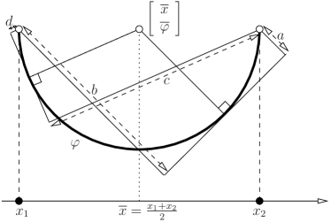
Figure 3: $\varphi$ is half-circle and ${\mathcal{S}}=\{x_{1},x_{2}\}$. In this case, all points in $[x_{1},x_{2}]$ are right population minimizers for $D_{\varphi,g_{\bot}}$ (the total Bregman divergence equals $a+b=c+d$).

Non-uniqueness and existence of the right population minimizers — The left population minimizer of any $v$-conformal divergence is unique (Lemma 1). This is not always the case for the right population minimizer. In very seldom but typical pathological cases, the population minimizers may even span the complete domain of $\varphi$, as displayed in Figure 3.

We also notice that the compactness of $\mathrm{dom}(D_{\varphi,g})$ appears necessary for the right population minimizers to exist, as otherwise one may build pathological Cauchy sequences for the right divergence parameter that converge to a right population minimizer not in $\mathrm{dom}(D_{\varphi,g})$.

Extension to scaled Bregman divergences — A new generalization of ordinary Bregman divergences has been recently coined [19], called scaled Bregman divergences. A scaled Bregman divergence is a particular case, for $g=v=\mathrm{Id}$, of what we call a scaled conformal divergence, defined as:

$$D^{v}_{\varphi,g}(x:y;w) \stackrel{{\scriptstyle\mathrm{.}}}{{=}} wD^{v}_{\varphi,g}(x/w:y/w)\>\>,$$ (69)

for $w>0$. A conformal divergence is obtained when $w=1$. Scaled Bregman divergences generalize other important classes of divergences such as Csiszár’s $f$-divergences, and they yield explicit formulas for exponential families for scaled Bregman power divergences, which means they have a significant potential for applications in clustering [19]. It is thus important to characterize their population minimizers. Though it is out of the scope of our paper to extent further our results to scaled divergences, we can give some insights into the similarities and differences with the case $w=1$. Population minimizers are now sought with respect to some sets $\mathcal{S}=\{x_{1},x_{2},...,x_{n}\}$ and $\mathcal{W}=\{w_{1},w_{2},...,w_{n}\}$, such that a left population minimizer of the ordered pair $(\mathcal{S},\mathcal{W})$ for $D^{v}_{\varphi,g}$ is defined as $\mu$ that minimizes $\sum_{i}D^{v}_{\varphi,g}(\mu:x_{i};w_{i})$. The following Lemma shows that, despite the left population minimizer is not always available in closed form in general (unlike $v$-conformal divergences), it is in between the minimal and maximal values of ${\mathcal{S}}$ (like $v$-conformal divergences).

Lemma 9

The left population minimizer of $D^{v}_{\varphi,g}$ over $(\mathcal{S},\mathcal{W})$ is unique and in $[\min_{i}x_{i},\max_{i}x_{i}]$.

(Proof in Appendix, Subsection 10.7) This Lemma can be extended to separable divergences in ${\mathbb{R}}^{d}$, to show that the left population minimizer of scaled conformal divergences lies in $\prod_{j}[\min_{i}x^{j}_{i},\max_{i}x^{j}_{i}]$.

8 Conclusion

We have studied the left and right population minimizers of conformal divergences, a superset of ordinary Bregman divergences and total Bregman divergences, in the $(u,v)_{\varphi}$-geometric structure [20, 21, 22], which generalizes dually flat affine connections. We have characterized analytically and geometrically the population minimizers, shown the exhaustivity property of conformal divergences for the left population minimizer, and the exhaustivity of total Bregman divergences for the right population minimizers. We do believe that these results, as well as additional results we provide on the robustness of the population minimizers, the nature of the $(u,v)_{\varphi}$ geometric structure relation, and the simple approximation of 1D population minimizers, shall be useful to widen the scope of existing clustering algorithms and/or develop algorithmically new clustering algorithms relying on broad classes of distortions that escape the conventional framework of ordinary Bregman divergences, as e.g. recently initiated with total Bregman divergences or scaled Bregman divergences.

9 Acknowledgments

The authors thank Meizhu Liu, and the reviewers for insightful comments that helped to significantly improve the paper.

10 Appendix

10.1 Proof of Lemma 1

Any left population minimizer $\bm{\mu}$ satisfies $\nabla\sum_{i}{D_{\varphi,g}^{v}(\bm{\mu}:\bm{x}_{i})}=\bm{0}$, and so, after simplification, we obtain:

$$J_{v}(\bm{\mu})\sum_{i}{g(\bm{x}_{i})\left(\nabla\varphi(v(\bm{\mu}))-\nabla\varphi(v(\bm{x}_{i}))\right)} = \bm{0}\>\>,$$ (70)

where $J_{v}$ is the Jacobian of $v$. Since $v$ is bijective, the null space of $J_{v}$ is reduced to $\{\bm{0}\}$, and so we must have:

$$\sum_{i}{g(\bm{x}_{i})\left(\nabla\varphi(v(\bm{\mu}))-\nabla\varphi(v(\bm{x}_{i}))\right)} = \bm{0}\>\>,$$

which, after solving for $\bm{\mu}$, yields:

$$\bm{\mu} = v^{-1}\nabla\varphi^{-1}\left(\frac{1}{\sum_{i}g(\bm{x}_{i})}\sum_{i}g(\bm{x}_{i})\nabla\varphi(v(\bm{x}_{i}))\right)\>\>.$$

There remains to use the $u$-coordinate mapping to obtain (8).

10.2 Proof of Lemma 2

Let $\bm{x}_{u}\stackrel{{\scriptstyle\mathrm{.}}}{{=}}u(\bm{x}),\forall\bm{x}$ and let ${\mathcal{S}}_{u}\stackrel{{\scriptstyle\mathrm{.}}}{{=}}\{(\bm{x}_{i})_{u},i=1,2,...,n\}$. We have $\bm{\mu}_{u}=\sum_{i}w_{i}(\bm{x}_{i})_{u}$ and

$$D(\bm{\mu}:\bm{x}_{i}) = D(u^{-1}(\bm{\mu}_{u}):u^{-1}((\bm{x}_{i})_{u}))$$ (71)

$$\stackrel{{\scriptstyle\mathrm{.}}}{{=}} D_{2}(\bm{\mu}_{u}:(\bm{x}_{i})_{u})\>\>.$$

From (71), the assumptions on $D$ and the properties of $u$, it follows that $D_{2}$ is non-negative, differentiable, satisfies $D_{2}(\bm{x}:\bm{x})=0,\forall\bm{x}$, and its left population minimizer over ${\mathcal{S}}_{u}$ is the weighted arithmetic average $\bm{\mu}_{u}$: it is thus an ordinary Bregman divergence [7] with:

$$D_{2}(\bm{\mu}_{u}:(\bm{x}_{i})_{u}) = w_{i}D_{\phi}((\bm{x}_{i})_{u}:\bm{\mu}_{u})\>\>,$$ (72)

for some strictly convex differentiable $\phi$. Calling to convex conjugates, we obtain:

$$D_{\phi}((\bm{x}_{i})_{u}:\bm{\mu}_{u})$$ (73)

$$= D_{\phi^{\star}}(\nabla\phi(\bm{\mu}_{u}):\nabla\phi((\bm{x}_{i})_{u}))$$

$$= D_{\phi^{\star}}((\nabla\phi\circ u)(\bm{\mu}):(\nabla\phi\circ u)(\bm{x}_{i}))$$

$$\stackrel{{\scriptstyle\mathrm{.}}}{{=}} D_{\varphi}(v(\bm{\mu}):v(\bm{x}_{i}))\>\>,$$

with $\varphi\stackrel{{\scriptstyle\mathrm{.}}}{{=}}\phi^{\star}$ and $(v,u)_{\phi}$-geometric structure. $(u,v)_{\varphi}$ is thus a geometric structure and merging (71 — 73), we obtain:

$$D(\bm{\mu}:\bm{x}_{i}) = w_{i}D_{\varphi}(v(\bm{\mu}):v(\bm{x}_{i}))\>\>.$$ (74)

$$= g(\bm{x}_{i})D_{\varphi}(v(\bm{\mu}):v(\bm{x}_{i}))\>\>,$$

for some $g$ admitting continuous directional derivatives which meets $g(\bm{x}_{i})=w_{i},\forall i=1,2,...,n$ (we can pick e.g. a degree-$n$ polynomial). We obtain (9), as claimed. This ends the proof of Lemma 2.

10.3 Proof of Lemma 3

The first part of the proof is standard, and shows that ${\mathbb{P}}_{{\mathcal{S}},\varphi,g}$ is the set of critical points for the right parameter [29]. Assume $\bm{\mu}$ is a population minimizer, and define $\mathrm{D}_{t,\bm{z}}D_{\varphi,g}({\mathcal{S}}:\bm{y})\stackrel{{\scriptstyle\mathrm{.}}}{{=}}\sum_{i}{\mathrm{D}_{t,\bm{z}}D_{\varphi,g}(\bm{x}_{i}:\bm{y})}$. Fix any valid direction $\bm{z}$. Because $\bm{\mu}$ is a right population minimizer, it comes $\mathrm{D}_{t,\bm{z}}D_{\varphi,g}({\mathcal{S}}:\bm{\mu})\leq 0$ for $t\leq 0$, and $\mathrm{D}_{t,\bm{z}}D_{\varphi,g}({\mathcal{S}}:\bm{\mu})\geq 0$ for $t\geq 0$. Since directional derivatives are defined in direction $\bm{z}$, we obtain $0\leq\lim_{t\downarrow 0}\mathrm{D}_{t,\bm{z}}D_{\varphi,g}({\mathcal{S}}:\bm{\mu})=\mathrm{D}_{\bm{z}}D_{\varphi,g}({\mathcal{S}}:\bm{\mu})=\lim_{t\uparrow 0}\mathrm{D}_{t,\bm{z}}D_{\varphi,g}({\mathcal{S}}:\bm{\mu})\leq 0$ and $\bm{\mu}$ is a solution of:

$$\lim_{t\rightarrow 0}\mathrm{D}_{t,\bm{z}}D_{\varphi,g}({\mathcal{S}}:\bm{\mu}) = \mathrm{D}_{\bm{z}}\sum_{i}D_{\varphi,g}(\bm{x}_{i}:\bm{\mu})$$ (75)

$$= 0\>\>.$$

We plug in (75) the expression of $D_{\varphi,g}$ and obtain that for any right population minimizer $\bm{\mu}$, the following holds:

$$\frac{1}{n}\mathrm{D}_{\bm{z}}\sum_{i}D_{\varphi,g}(\bm{x}_{i}:\bm{\mu})$$ (76)

$$= \mathrm{D}_{\bm{z}}g(\bm{\mu})\times\frac{1}{n}\sum_{i}D_{\varphi}(\bm{x}_{i}:\bm{\mu})$$

$$+g(\bm{\mu})(\bm{\mu}-\overline{\bm{x}})^{\top}\mathrm{H}\varphi(\bm{\mu})\bm{z}$$

$$= 0\>\>.$$

Rewriting, we thus need:

$$\mathrm{D}_{\bm{z}}g(\bm{\mu})\times(\overline{\varphi}-\varphi(\bm{\mu}))$$

$$= (\overline{\bm{x}}-\bm{\mu})^{\top}(g(\bm{\mu})\mathrm{H}\varphi(\bm{\mu})\bm{z}$$

$$+\mathrm{D}_{\bm{z}}g(\bm{\mu})\nabla\varphi(\bm{\mu}))$$

$$= (\overline{\bm{x}}-\bm{\mu})^{\top}\mathrm{D}_{\bm{z}}(g(\bm{\mu})\nabla\varphi(\bm{\mu}))\>\>,$$

which implies $\bm{\mu}\in{\mathbb{P}}_{{\mathcal{S}},\varphi,g}$. If a population minimizer does not belong to ${\mathbb{P}}_{{\mathcal{S}},\varphi,g}$, it is in the non differentiable part of the boundary, that is, in ${\mathbb{B}}_{\varphi,g}$. Eq. (10.3) brings:

$$\mathrm{D}_{\bm{z}}g(\bm{\mu})\times\frac{1}{n}\sum_{i}D_{\varphi}(\bm{x}_{i}:\bm{\mu})$$

$$= g(\bm{\mu})\times(\overline{\bm{x}}-\bm{\mu})^{\top}\mathrm{H}\varphi(\bm{\mu})\bm{z}\>\>,$$

and so:

$$\frac{1}{n}\sum_{i}D_{\varphi,g}(\bm{x}_{i}:\bm{\mu})$$ (78)

$$= \frac{(\overline{\bm{x}}-\bm{\mu})^{\top}\mathrm{H}\varphi(\bm{\mu})\bm{z}}{\mathrm{D}_{\bm{z}}g(\bm{\mu})}g^{2}(\bm{\mu})\>\>,$$

a quantity which does not depend on the direction $\bm{z}\neq\bm{0}$. Fixing as direction $\bm{z}=\overline{\bm{x}}-\bm{\mu}$ yields the statement of (24).

10.4 Proof of Theorem 1

We first need the following Lemma.

Lemma 10

Suppose $g(\bm{x})=f(\nabla\varphi(\bm{x}))$, with $\varphi$ strictly convex twice differentiable and $f$ differentiable. $\forall\bm{\mu}\in{\mathbb{P}}_{{\mathcal{S}},\varphi,g}$, we have:

$$\overline{\bm{x}}-\bm{\mu}$$ (79)

$$= \frac{1}{f(\nabla\varphi(\bm{\mu}))}\left(\frac{1}{n}\sum_{i}D_{\varphi}(\bm{x}_{i}:\bm{\mu})\right)$$

$$\cdot\nabla f(\nabla\varphi(\bm{\mu}))\>\>.$$

Proof:

The chain rule gives

$$\mathrm{D}_{\bm{z}}g(\bm{\mu}) = \mathrm{D}_{\bm{z}}(f(\nabla\varphi(\bm{\mu})))$$

$$= \mathrm{D}_{\mathrm{D}_{\bm{z}}\nabla\varphi(\bm{\mu})}f(\nabla\varphi)$$

$$= \mathrm{D}_{\mathrm{H}\varphi(\bm{\mu})\bm{z}}f(\nabla\varphi)$$

$$= \bm{z}^{\top}(\mathrm{H}\varphi(\bm{\mu}))^{\top}\nabla f(\nabla\varphi(\bm{\mu}))$$

$$= \bm{z}^{\top}\mathrm{H}\varphi(\bm{\mu})\nabla f(\nabla\varphi(\bm{\mu}))\>\>,$$

so that (10.3) becomes:

$$\bm{z}^{\top}\mathrm{H}\varphi(\bm{\mu})\left((\overline{\varphi}-\varphi(\bm{\mu}))\times\nabla f(\nabla\varphi(\bm{\mu}))\right)$$ (83)

$$= \bm{z}^{\top}\mathrm{H}\varphi(\bm{\mu})\left(g(\bm{\mu})\times(\overline{\bm{x}}-\bm{\mu})\right)$$

$$+\bm{z}^{\top}\mathrm{H}\varphi(\bm{\mu})\left(\nabla\varphi(\bm{\mu})^{\top}(\overline{\bm{x}}-\bm{\mu})\times\nabla f(\nabla\varphi(\bm{\mu}))\right)$$

$$= \bm{z}^{\top}\mathrm{H}\varphi(\bm{\mu})\left(\begin{array}[]{c}g(\bm{\mu})\times(\overline{\bm{x}}-\bm{\mu})\\ +\\ \nabla\varphi(\bm{\mu})^{\top}(\overline{\bm{x}}-\bm{\mu})\times\nabla f(\nabla\varphi(\bm{\mu}))\end{array}\right)\>\>.$$

Eq. (83) is of the form $\bm{z}^{\top}\mathrm{H}\varphi(\bm{\mu})\bm{a}=\bm{z}^{\top}\mathrm{H}\varphi(\bm{\mu})\bm{b}$ which implies $\bm{a}=\bm{b}$ as otherwise picking $\bm{z}=\bm{b}-\bm{a}\neq\bm{0}$ would contradict the positive definiteness of the Hessian $\mathrm{H}\varphi$. After reordering, we get eq. (79). This ends the proof of Lemma 10.       ∎

(Continued proof of Theorem 1) Let us fix $f(\bm{x})=f_{p}(\bm{x})\stackrel{{\scriptstyle\mathrm{.}}}{{=}}1/(1+\|\bm{x}\|_{p}^{p})^{1/p}$. We have:

$$\nabla f(\nabla\varphi(\bm{\mu})) = -\frac{1}{(1+\|\nabla\varphi(\bm{\mu})\|_{p}^{p})^{1+\frac{1}{p}}}\nabla_{p}\varphi(\bm{\mu})\>\>,$$ (84)

where $\nabla_{p}\varphi(\bm{\mu})$ is the vector whose $j^{th}$ coordinate is $\mathrm{sign}(\nabla^{j})|\nabla^{j}|^{p-1}$, where $\nabla^{j}$ is coordinate $j$ of $\nabla\varphi(\bm{\mu})$. This definition brings the following relationship:

$$\nabla\varphi(\bm{\mu})^{\top}\nabla_{p}\varphi(\bm{\mu}) = \|\nabla\varphi(\bm{\mu})\|_{p}^{p}\>\>.$$ (85)

We now use (79) with $f=f_{p}$ and obtain:

$$\overline{\bm{x}}-\bm{\mu} = -\frac{1}{1+\|\nabla\varphi(\bm{\mu})\|_{p}^{p}}\left(\frac{1}{n}\sum_{i}D_{\varphi}(\bm{x}_{i}:\bm{\mu})\right)$$ (86)

$$\times\nabla_{p}\varphi(\bm{\mu})\>\>.$$

Coordinate $j$ in $\overline{\bm{x}}-\bm{\mu}$, $(\overline{\bm{x}}-\bm{\mu})^{j}$, satisfies:

$$((\overline{\bm{x}}-\bm{\mu})^{j})^{q-1}$$ (87)

$$= \left(\frac{-m}{1+\|\nabla\varphi(\bm{\mu})\|_{p}^{p}}\right)^{q-1}\times(\mathrm{sign}(\nabla^{j})|\nabla^{j}|^{p-1})^{q-1}$$

$$= -\left(\frac{m}{1+\|\nabla\varphi(\bm{\mu})\|_{p}^{p}}\right)^{q-1}\times\nabla^{j}\>\>,$$

where $m\stackrel{{\scriptstyle\mathrm{.}}}{{=}}(1/m)\sum_{i}D_{\varphi}(\bm{x}_{i}:\bm{\mu})\geq 0$. Eq. (87) holds because $(p-1)(q-1)=1$ and $q=2k\in{\mathbb{N}}$ is even. So, we may write:

$$\|\overline{\bm{x}}-\bm{\mu}\|_{q}^{q}$$ (88)

$$\stackrel{{\scriptstyle\mathrm{.}}}{{=}} \sum_{j}{((\overline{\bm{x}}-\bm{\mu})^{j})^{q}}$$

$$= \sum_{j}{((\overline{\bm{x}}-\bm{\mu})^{j})^{q-1}\times(\overline{\bm{x}}-\bm{\mu})^{j}}$$

$$= -\left(\frac{m}{1+\|\nabla\varphi(\bm{\mu})\|_{p}^{p}}\right)^{q-1}\times(\overline{\bm{x}}-\bm{\mu})^{\top}\nabla\varphi(\bm{\mu})\>\>.$$

We make the inner product of (86) with $\nabla\varphi(\bm{\mu})$ and obtain because of (85):

$$(\overline{\bm{x}}-\bm{\mu})^{\top}\nabla\varphi(\bm{\mu})$$ (89)

$$= -\frac{\|\nabla\varphi(\bm{\mu})\|_{p}^{p}}{1+\|\nabla\varphi(\bm{\mu})\|_{p}^{p}}\left(\frac{1}{n}\sum_{i}D_{\varphi}(\bm{x}_{i}:\bm{\mu})\right)\>\>,$$

$$= -\alpha(\overline{\varphi}-\varphi(\bm{\mu}))+\alpha(\overline{\bm{x}}-\bm{\mu})^{\top}\nabla\varphi(\bm{\mu})\>\>,$$

with $\alpha\stackrel{{\scriptstyle\mathrm{.}}}{{=}}\|\nabla\varphi(\bm{\mu})\|_{p}^{p}/(1+\|\nabla\varphi(\bm{\mu})\|_{p}^{p})$. We obtain $-(1-\alpha)(\overline{\bm{x}}-\bm{\mu})^{\top}\nabla\varphi(\bm{\mu})=\alpha(\overline{\varphi}-\varphi(\bm{\mu}))$, that is, after adding $(1-\alpha)(\overline{\varphi}-\varphi(\bm{\mu}))$ on both sides:

$$\overline{\varphi}-\varphi(\bm{\mu})$$ (90)

$$= \frac{1}{1+\|\nabla\varphi(\bm{\mu})\|_{p}^{p}}\left(\frac{1}{n}\sum_{i}D_{\varphi}(\bm{x}_{i}:\bm{\mu})\right)\>\>.$$

We finally get from (88) and (90), using the shorthand $m\stackrel{{\scriptstyle\mathrm{.}}}{{=}}(1/n)\sum_{i}D_{\varphi}(\bm{x}_{i}:\bm{\mu})$:

$$\|\overline{\bm{x}}^{+}-\bm{\mu}^{+}\|_{q}$$

$$= \left(|\overline{\varphi}-\varphi(\bm{\mu})|^{q}+\|\overline{\bm{x}}-\bm{\mu}\|_{q}^{q}\right)^{\frac{1}{q}}$$

$$= \left((\overline{\varphi}-\varphi(\bm{\mu}))^{q-1}\times(\overline{\varphi}-\varphi(\bm{\mu}))+\|\overline{\bm{x}}-\bm{\mu}\|_{q}^{q}\right)^{\frac{1}{q}}$$

$$= \left(\begin{array}[]{c}\left(\frac{m}{1+\|\nabla\varphi(\bm{\mu})\|_{p}^{p}}\right)^{q-1}(\overline{\varphi}-\varphi(\bm{\mu}))\\ -\\ \left(\frac{m}{1+\|\nabla\varphi(\bm{\mu})\|_{p}^{p}}\right)^{q-1}(\overline{\bm{x}}-\bm{\mu})^{\top}\nabla\varphi(\bm{\mu})\end{array}\right)^{\frac{1}{q}}$$

$$= \frac{m^{\frac{1}{p}}}{(1+\|\nabla\varphi(\bm{\mu})\|_{p}^{p})^{\frac{1}{p}}}$$

$$\times\left(\overline{\varphi}-\varphi(\bm{\mu})-(\overline{\bm{x}}-\bm{\mu})^{\top}\nabla\varphi(\bm{\mu})\right)^{\frac{1}{q}}$$

$$= \frac{m^{\frac{1}{p}+\frac{1}{q}}}{(1+\|\nabla\varphi(\bm{\mu})\|_{p}^{p})^{\frac{1}{p}}}$$

$$= \frac{m}{(1+\|\nabla\varphi(\bm{\mu})\|_{p}^{p})^{\frac{1}{p}}}$$

$$= \frac{1}{n}\sum_{i}D_{\varphi,g_{p}}(\bm{x}_{i}:\bm{\mu})$$

$$= \frac{1}{K}\times\left(\frac{1}{n}\sum_{i}D_{\varphi,Kg_{p}}(\bm{x}_{i}:\bm{\mu})\right)\>\>,$$

which yields the statement of Theorem 1.

10.5 Proof of Lemma 6

Clearly, $(u,u)$ holds since $(u,u)_{\varphi}$ is a geometric structure for $\varphi\stackrel{{\scriptstyle\mathrm{.}}}{{=}}(1/2)\sum_{i}(x^{i})^{2}$ so the relation is reflexive. If $(u,v)_{\varphi}$ is a geometric structure, then $(v,u)_{\varphi^{\star}}$ is a geometric structure, so the relation is symmetric, which completes the proof that $(u,v)$ is a tolerance relation.

Let $(u,v)_{\varphi}$ and $(v,w)_{\phi}$ be two geometric structures. We have $u\circ w^{-1}=\nabla\varphi\circ\nabla\phi$, and so $J_{u\circ w^{-1}}=\mathrm{H}\varphi(\nabla\phi)\mathrm{H}\phi$, that we want to be symmetric positive definite for the “geometric structure” relation to be transitive. Both $\mathrm{H}\varphi$ and $\mathrm{H}\phi$ are symmetric positive definite. Since (i) the product of two positive definite matrices is positive definite iff their product is normal, and (ii) the product of two symmetric matrices is symmetric iff their have the same eigenspace, it follows that $\mathrm{H}\varphi(\nabla\phi)\mathrm{H}\phi\succ 0$ iff we have the diagonalizations $\mathrm{H}\varphi(\nabla\phi)=PD_{1}P^{\top}$ and $\mathrm{H}\phi=PD_{2}P^{\top}$, with $P$ unitary and $D_{1},D_{2}\succ 0$. This finishes the proof of Lemma 6.

10.6 Proof of Lemma 8

We suppose without loss of generality that $K=1$. The proof relies on the study in $[x_{1},x_{n}]$ of function $\tilde{\varphi}^{\prime}_{\bot}(x)\stackrel{{\scriptstyle\mathrm{.}}}{{=}}-1/\tilde{\varphi}^{\prime}_{\mathcal{S}}(x)$ (see eq. (36)), which is the slope of the line orthogonal to the segment which links $(\overline{x},\overline{\varphi})$ to $(\overline{x},\varphi(\overline{x}))$.

Suppose $\varphi^{\prime}(x)$ is $<0$ on $[x_{1},x_{n}]$, which implies $\varphi(x_{1})\geq\overline{\varphi}$, and so $\overline{x}_{\varphi}\in[x_{1},\overline{x}]$, and satisfies $\varphi(\overline{x}_{\varphi})=\overline{\varphi}$. It comes $\tilde{\varphi}^{\prime}_{\bot}(x)\leq 0$ on $(\overline{x}_{\varphi},\overline{x}]$, with $\lim_{x\downarrow\overline{x}_{\varphi}}\tilde{\varphi}^{\prime}_{\bot}(x)=-\infty$ and $\tilde{\varphi}^{\prime}_{\bot}(\overline{x})=0$. Because $\tilde{\varphi}^{\prime}_{\mathcal{S}}(x)$ is continuous, so is $\tilde{\varphi}^{\prime}_{\bot}(x)$ and so there must be $\mu\in(\overline{x}_{\varphi},\overline{x}]$ such that $\tilde{\varphi}^{\prime}_{\bot}(\mu)=\varphi^{\prime}(x)$. This $\mu$ is a candidate right population minimizer.

Suppose now that $\varphi^{\prime}(x)$ is $>0$ on $[x_{1},x_{n}]$, which implies $\varphi(x_{n})\geq\overline{\varphi}$, and so $\overline{x}_{\varphi}\in[\overline{x},x_{n}]$, and satisfies $\varphi(\overline{x}_{\varphi})=\overline{\varphi}$. This time, $\tilde{\varphi}^{\prime}_{\bot}(\overline{x})=0$ and $\lim_{x\uparrow\overline{x}_{\varphi}}\tilde{\varphi}^{\prime}_{\bot}(x)=+\infty$, so there must be $\mu\in[\overline{x},\overline{x}_{\varphi})$ such that $\tilde{\varphi}^{\prime}_{\bot}(\mu)=\varphi^{\prime}(x)$. This $\mu$ is a candidate right population minimizer. This ends the proof of Lemma 8.

10.7 Proof of Lemma 9

We build upon eq. (70). Any left population minimizer is a solution of:

$$0=\frac{\mathrm{d}}{\mathrm{d}\mu}\sum_{i}w_{i}D^{v}_{\varphi,g}(\mu/w_{i}:x_{i}/w_{i})$$ (95)

$$= \sum_{i}g\left({\frac{x_{i}}{w_{i}}}\right)v^{\prime}\left({\frac{\mu}{w_{i}}}\right)\left({u\left({\frac{\mu}{w_{i}}}\right)-u\left({\frac{x_{i}}{w_{i}}}\right)}\right)$$

$$= \sum_{i}g\left({\frac{x_{i}}{w_{i}}}\right)v^{\prime}\left({\frac{\mu}{w_{i}}}\right)\left({\frac{\mu-x_{i}}{w_{i}}}\right)u^{\prime}\left({\frac{\mu_{i}}{w_{i}}}\right)\>\>.$$

where $\mu_{i}\stackrel{{\scriptstyle\mathrm{.}}}{{=}}\mu+\alpha_{i}(x_{i}-\mu)$ for some $0<\alpha_{i}<1$. Eq (95) is obtained after $n$ Taylor expansions of $u$. We also have $(v\circ u^{-1})^{\prime}=(v^{\prime}\circ u^{-1})/(u^{\prime}\circ u^{-1})\stackrel{{\scriptstyle\mathrm{.}}}{{=}}(\varphi^{\star})^{\prime\prime}$, and so, since $\varphi^{\star}$ is strictly convex, $v^{\prime}(x)$ and $u^{\prime}(x)$ have the same sign. Since $u$ is strictly monotonous, $u^{\prime}$ does not change sign over its domain, and so the product $\pi_{i}\stackrel{{\scriptstyle\mathrm{.}}}{{=}}g\left({x_{i}/w_{i}}\right)v^{\prime}\left({\mu/w_{i}}\right)u^{\prime}\left({\mu_{i}/w_{i}}\right)$ is non negative, $\forall i$. We can summarize (95) as $h(\mu)\stackrel{{\scriptstyle\mathrm{.}}}{{=}}\sum_{i}\pi_{i}(\mu-x_{i})/w_{i}=0$: since all $w_{i}>0$, we get $h(\min_{i}x_{i})\leq 0$ and $h(\max_{i}x_{i})\geq 0$. Since each summand in $h$ is the product of continuous functions, there must be $\mu\in[\min_{i}x_{i},\max_{i}x_{i}]$ such that (95) holds, and since $h$ is strictly increasing, there is only one such point. Since $\sum_{i}D_{\varphi,g}(\mu:x_{i};w_{i})$ is strictly convex in $\mu$, this is the left population minimizer. This ends the proof of Lemma 9.

  

These subsections present the additional proofs not in the published paper.

  

10.8 Proof of Theorem 2

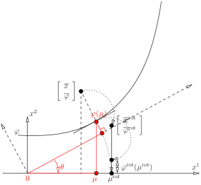
Figure 4: We perform a rotation of angle $\theta$ on $\varphi$ such that, after rotation, $\varphi^{\prime\mathrm{rot}}(\mu^{\mathrm{rot}})=0$, implying that $\overline{x}^{rot}$ is a population minimizer in ${\mathbb{P}}_{{\mathcal{S}}^{\mathrm{rot}},\varphi^{\mathrm{rot}}}$.

We distinguish two cases, first assuming that $\overline{x}\not\in{\mathbb{P}}_{{\mathcal{S}},\varphi}$. As shown in Figure 4, we perform a rotation of angle $\theta$ chosen so that $(1/n)\sum_{i}{\mathrm{M}_{\theta}\bm{x}^{+}_{i}}=\mathrm{M}_{\theta}((1/n)\sum_{i}{\bm{x}^{+}_{i}})=\mathrm{M}_{\theta}\overline{\bm{x}}^{+}=\mathrm{M}_{\theta}\bm{\mu}^{+}$, with

$$\mathrm{M}_{\theta} \stackrel{{\scriptstyle\mathrm{.}}}{{=}} \left[\begin{array}[]{cc}\cos\theta&-\sin\theta\\ \sin\theta&\cos\theta\end{array}\right]\>\>,$$ (98)

$$\bm{x}^{+}_{i} \stackrel{{\scriptstyle\mathrm{.}}}{{=}} \left[\begin{array}[]{c}x_{i}\\ \varphi(x_{i})\end{array}\right]\>\>,$$ (101)

and $\overline{\bm{x}}^{+}$ and $\bm{\mu}^{+}$ are defined in (15) and (18). So, the population minimizer of ${\mathcal{S}}$ after rotation is just the average, which implies, since the distortion is invariant to rotation after assumption (iii) and satisfies (i) and (ii), that the distortion equals an ordinary Bregman divergence computed after rotation, $D_{\phi^{\mathrm{rot}}}$, for some convex differentiable $\phi^{\mathrm{rot}}:{\mathbb{R}}\rightarrow{\mathbb{R}}$ [7, 8]. We then get:

$$D(x:\mu)$$ (102)

$$= D((\mathrm{M}_{\theta}\bm{x}^{+})^{1}:(\mathrm{M}_{\theta}\bm{\mu}^{+})^{1})$$

$$= D_{\phi^{\mathrm{rot}}}((\mathrm{M}_{\theta}\bm{x}^{+})^{1}:(\mathrm{M}_{\theta}\overline{\bm{x}}^{+})^{1})$$

$$= \phi^{\mathrm{rot}}((\mathrm{M}_{\theta}\bm{x}^{+})^{1})-\phi^{\mathrm{rot}}((\mathrm{M}_{\theta}\overline{\bm{x}}^{+})^{1})$$

$$-((\mathrm{M}_{\theta}\bm{x}^{+})^{1}-(\mathrm{M}_{\theta}\overline{\bm{x}}^{+})^{1})\phi^{\prime\mathrm{rot}}((\mathrm{M}_{\theta}\overline{\bm{x}}^{+})^{1})\>\>$$

(exponent “1” refers to the $x$-coordinate). Let us denote $\phi:{\mathbb{R}}^{d}\rightarrow{\mathbb{R}}$ the function obtained from $\phi^{\mathrm{rot}}$ by rotation $\mathrm{M}_{\theta}$ of the curve. We have:

$$\phi^{\mathrm{rot}}((\mathrm{M}_{\theta}\bm{x}^{+})^{1}) = (\mathrm{M}_{\theta}\bm{x}^{+})^{2}=x\sin\theta+\phi(x)\cos\theta\>\>,$$

$$\phi^{\mathrm{rot}}((\mathrm{M}_{\theta}\overline{\bm{x}}^{+})^{1}) = (\mathrm{M}_{\theta}\overline{\bm{x}}^{+})^{2}=\mu\sin\theta+\phi(\mu)\cos\theta\>\>$$

(exponent “2” refers here to the $y$-coordinate), and

$$((\mathrm{M}_{\theta}\bm{x}^{+})^{1}-(\mathrm{M}_{\theta}\overline{\bm{x}}^{+})^{1})\phi^{\prime\mathrm{rot}}((\mathrm{M}_{\theta}\overline{\bm{x}}^{+})^{1})$$

$$= (x\cos\theta-\phi(x)\sin\theta-\mu\cos\theta+\phi(\mu)\sin\theta)$$

$$\times\frac{\sin\theta+\phi^{\prime}(\mu)\cos\theta}{\cos\theta-\phi^{\prime}(\mu)\sin\theta}\>\>.$$

Eq. (102) thus becomes $D(x:\mu)=Q+R$, with $Q\stackrel{{\scriptstyle\mathrm{.}}}{{=}}(\phi(x)-\phi(\mu))\cos\theta$, and:

$$R$$ (105)

$$\stackrel{{\scriptstyle\mathrm{.}}}{{=}} (x-\mu)\sin\theta$$

$$-\left\{\begin{array}[]{c}x\cos\theta-\phi({x})\sin\theta\\ -\mu\cos\theta+\phi({\mu})\sin\theta\end{array}\right\}\times\frac{\sin\theta+\phi^{\prime}(\mu)\cos\theta}{\cos\theta-\phi^{\prime}(\mu)\sin\theta}$$

$$= \frac{\left\{\begin{array}[]{c}x\sin\theta\cos\theta-x\phi^{\prime}(\mu)\sin^{2}\theta\\ -\mu\sin\theta\cos\theta+\mu\phi^{\prime}(\mu)\sin^{2}\theta\\ -x\sin\theta\cos\theta-x\phi^{\prime}(\mu)\cos^{2}\theta\\ +\mu\sin\theta\cos\theta+\mu\phi^{\prime}(\mu)\cos^{2}\theta\\ +(\phi({x})-\phi({\mu}))\sin\theta(\sin\theta+\phi^{\prime}(\mu)\cos\theta)\end{array}\right\}}{\cos\theta-\phi^{\prime}(\mu)\sin\theta}$$ (111)

$$= \frac{\left\{\begin{array}[]{c}-(x-\mu)\phi^{\prime}(\mu)\\ +(\phi({x})-\phi({\mu}))(1-\cos^{2}\theta+\phi^{\prime}(\mu)\sin\theta\cos\theta)\end{array}\right\}}{\cos\theta-\phi^{\prime}(\mu)\sin\theta}$$

$$= \frac{\phi({x})-\phi({\mu})-(x-\mu)\phi^{\prime}(\mu)}{\cos\theta-\phi^{\prime}(\mu)\sin\theta}$$

$$-(\phi({x})-\phi({\mu}))\cos\theta\>\>.$$

We thus get:

$$D({x}:{\mu}) = \frac{\phi({x})-\phi({\mu})-(x-\mu)\phi^{\prime}(\mu)}{\cos\theta-\phi^{\prime}(\mu)\sin\theta}$$ (115)

$$= D_{\phi,g}(x:\mu)\>\>,$$

with

$$g({\mu}) \stackrel{{\scriptstyle\mathrm{.}}}{{=}} \frac{\sqrt{1+\varphi^{\prime}({\mu})^{2}}}{1+\phi^{\prime}(\mu)\varphi^{\prime}({\mu})}\>\>,$$ (116)

as indeed $\cos\theta=1/\sqrt{1+\varphi^{\prime}({\mu})^{2}}$ and $\sin\theta=-\varphi^{\prime}(\mu)/\sqrt{1+\varphi^{\prime}({\mu})^{2}}$.

Eqs (115) and (116) are the consequences of assumptions (i-iv). On the other hand, assumption (iv) and (34) imply for right population minimizer $\mu$ of set ${\mathcal{S}}$:

$$-\varphi^{\prime}(\mu)(\overline{\varphi}-\varphi(\mu)) = (\overline{x}-\mu)\>\>.$$ (117)

Since $\overline{x}\neq\mu$, we obtain $\varphi^{\prime}(\mu)\neq 0$, so we can replace $\varphi^{\prime}(\mu)$ in (116) by its expression from (117) and obtain:

$$g(\mu) = \frac{\sqrt{1+\left(\frac{\overline{x}-\mu}{\overline{\varphi}-\varphi(\mu)}\right)^{2}}}{1-\phi^{\prime}(\mu)\times\left(\frac{\overline{x}-\mu}{\overline{\varphi}-\varphi(\mu)}\right)}$$

$$= \frac{\sqrt{(\overline{\varphi}-\varphi(\mu))^{2}+(\overline{x}-\mu)^{2}}}{\overline{\varphi}-\varphi(\mu)-(\overline{x}-\mu)\phi^{\prime}(\mu)}$$

$$= \frac{\|\overline{\bm{x}}^{+}-\bm{\mu}^{+}\|_{2}}{\overline{\varphi}-\varphi(\mu)-(\overline{x}-\mu)\phi^{\prime}(\mu)}\>\>,$$

where $\overline{\bm{x}}^{+}$ and $\bm{\mu}^{+}$ are defined in (15) and (18). For any ${\mathcal{S}}$ whose right population minimizer on $D_{\phi,g}$ is $\mu$, we get:

$$\frac{1}{n}\sum_{i}D({x}_{i}:{\mu})$$ (118)

$$= \|\overline{\bm{x}}^{+}-\bm{\mu}^{+}\|_{2}\times\frac{\overline{\phi}-\phi(\mu)-(\overline{x}-\mu)\phi^{\prime}(\mu)}{\overline{\varphi}-\varphi(\mu)-(\overline{x}-\mu)\phi^{\prime}(\mu)}$$

Because of assumption (iii), we want (118) to be invariant to rotation of the axes. Only term $\|\overline{\bm{x}}^{+}-\bm{\mu}^{+}\|_{2}$ is invariant because of assumption (iv). Both the numerator and the denominator after the times in (118) are not invariant to rotation. To have their ratio invariant, it must therefore be independent from the choice of ${\mathcal{S}}$, and thus constant, so we have:

$$\overline{\phi}-\phi(\mu)-(\overline{x}-\mu)\phi^{\prime}(\mu)$$

$$= K(\overline{\varphi}-\varphi(\mu)-(\overline{x}-\mu)\phi^{\prime}(\mu))\>\>,$$

Taking the derivative in some $x_{i}$ yields $\phi^{\prime}(x_{i})=K\varphi^{\prime}(x_{i})-(K-1)x_{i}\phi^{\prime}(\mu)$, which implies that the right hand side is independent of $\mu$, and since $\phi^{\prime}$ cannot always be zero, we obtain $K=1$, and so:

$$\phi = \varphi+\mathrm{constant}\>\>.$$ (119)

We obtain $D_{\phi,g}=D_{\varphi,g_{\bot}}$, and this completes the proof when $\overline{x}\not\in{\mathbb{P}}_{{\mathcal{S}},\varphi}$.

If $\overline{x}\in{\mathbb{P}}_{{\mathcal{S}},\varphi}$ is the population minimizer, then $D(x:\mu)=D(x:\overline{x})$ is an ordinary Bregman divergence [7, 8], say $D_{\phi}$ for some $\phi$ strictly convex twice differentiable. Because of assumption (iii), it comes in this case:

$$D(x:y) = \sqrt{\frac{1+\phi^{\prime}(\overline{x})^{2}}{1+\phi^{\prime}(y)^{2}}}D_{\phi}(x:y)$$

$$= \frac{K}{\sqrt{1+\phi^{\prime}(y)^{2}}}D_{\phi}(x:y)=D_{\phi,Kg_{\bot}}(x:y)\>\>.$$

Because of assumption (iv) and Lemma 1, $\phi^{\prime}=\varphi^{\prime}$ and so $\phi=\varphi+\mathrm{constant}$. This completes the proof in this second case, and completes the proof of Theorem 2.

11 Proof of Lemma 4

We use Lemma 1, and we fix ${\mathcal{S}}$ satisfying assumption (i). The left population minimizers $\bm{\mu}$ and $\bm{\mu}_{*}$ satisfy:

$$u(\bm{\mu}) = \frac{1}{\Sigma}\sum_{i}g(\bm{x}_{i})u(\bm{x}_{i})\>\>,$$

$$u(\bm{\mu}_{*}) = \frac{1-\epsilon}{\Sigma_{*}}\sum_{i}g(\bm{x}_{i})u(\bm{x}_{i})+\frac{\epsilon g(\bm{x}_{*})}{\Sigma_{*}}u(\bm{x}_{*})$$

$$= \frac{(1-\epsilon)\Sigma}{\Sigma_{*}}u(\bm{\mu})+\frac{\epsilon g(\bm{x}_{*})}{\Sigma_{*}}u(\bm{x}_{*})$$

$$= u(\bm{\mu})+\underbrace{\frac{\epsilon g(\bm{x}_{*})}{\Sigma_{*}}\left(u(\bm{x}_{*})-u(\bm{\mu})\right)}_{\epsilon\bm{\delta}}\>\>,$$

where $\Sigma\stackrel{{\scriptstyle\mathrm{.}}}{{=}}\sum_{i}g(\bm{x}_{i})$ and $\Sigma_{*}\stackrel{{\scriptstyle\mathrm{.}}}{{=}}(1-\epsilon)\Sigma+\epsilon g(\bm{x}_{*})$. Now, a Taylor expansion of $u^{-1}$ brings:

$$\bm{\mu}_{*}=u^{-1}\left(u(\bm{\mu})+\epsilon\bm{\delta}\right) = \bm{\mu}+\epsilon J_{u^{-1}}(\bm{\mu}_{\alpha})\bm{\delta}\>\>,$$

for some $\bm{\mu}_{\alpha}=u(\bm{\mu})+\alpha\epsilon\bm{\delta}$ with $0<\alpha<1$. We also have $J_{u^{-1}}(\bm{\mu}_{\alpha})=J^{-1}_{u}(u^{-1}(\bm{\mu}_{\alpha}))$, which, since $\bm{\mu}_{*}-\bm{\mu}=\epsilon\bm{\delta}_{\bm{\mu}}$, yields the influence function of $\bm{x}_{*}$:

$$\bm{\delta}_{\bm{\mu}} = \frac{g(\bm{x}_{*})}{\Sigma_{*}}\times J^{-1}_{u}(u^{-1}(\bm{\mu}_{\alpha}))\left(u(\bm{x}_{*})-u(\bm{\mu})\right)\>\>.$$ (120)

Let $J_{u}$ denote $J_{u}(u^{-1}(\bm{\mu}_{\alpha}))$ for short. Eq. (120) brings

$$\|\bm{\delta}_{\bm{\mu}}\|_{2}^{2} = \bm{\delta}^{\top}(J_{u}^{-1})^{\top}J_{u}^{-1}\bm{\delta}\leq\|\bm{\delta}\|_{2}^{2}\lambda_{\mathrm{max}}\>\>,$$ (121)

for some upperbound $\lambda_{\mathrm{max}}$ on the eigenvalues of $(J_{u}^{-1})^{\top}J_{u}^{-1}$. We also have

$$\|\bm{\delta}\|_{2}^{2} = \frac{g(\bm{x}_{*})}{\Sigma_{*}}\times\left\|u(\bm{x}_{*})-u(\bm{\mu})\right\|_{2}^{2}$$

$$\leq \frac{2g(\bm{x}_{*})}{\Sigma_{*}}\times(\|u(\bm{x}_{*})\|_{2}^{2}+\|u(\bm{\mu})\|_{2}^{2})$$

$$=\underbrace{\frac{2g(\bm{x}_{*})\|u(\bm{x}_{*})\|_{2}^{2}}{\Sigma_{*}}}_{a}+\underbrace{\frac{2g(\bm{x}_{*})\|u(\bm{\mu})\|_{2}^{2}}{\Sigma_{*}}}_{b}\>\>.$$

Because $\epsilon<1-\tau$, we have $\Sigma_{*}\geq\tau g(\bm{x}_{1})\stackrel{{\scriptstyle\mathrm{.}}}{{=}}K_{1}$ for some $K_{1}>0$ which does not depend upon $\bm{x}_{*}$ or $\epsilon$. Because of assumption (i), $g(\bm{x}_{*})\leq K_{2}$ for some constant $K_{2}>0$ and so $b=\tilde{O}(1)$ (the tilda meaning that the function does not depend upon $\bm{x}_{*}$ or $\epsilon$). Because of assumption (ii), $g(\bm{x}_{*})\|u(\bm{x}_{*})\|_{2}\leq K_{3}$ for some constant $K_{3}>0$ and so $a=\tilde{O}(1)$. Hence, $\|\bm{\delta}\|_{2}^{2}=\tilde{O}(1)$. There remains to plug this into (121), and remark that $\lambda_{\mathrm{max}}\leq 1/\lambda$ from assumption (iii), to conclude.

12 Proof of Lemma 5

The proof of this Lemma relies on the following Taylor expansions:

$$v(\bm{\mu}+\epsilon\bm{\delta}_{\bm{\mu}}) = v(\bm{\mu})+\epsilon J_{v}\bm{\delta}_{\bm{\mu}}\>\>,$$ (122)

for some value $J_{v}$ of the Jacobian of $v$ in between $\bm{\mu}$ and $\bm{\mu}+\epsilon\bm{\delta}_{\bm{\mu}}$,

$$v(\bm{x}_{*}) = v(\bm{\mu})+J^{\prime}_{v}(\bm{x}_{*}-\bm{\mu})\>\>,$$ (123)

for some value $J^{\prime}_{v}$ of the Jacobian of $v$ in between $\bm{\mu}$ and $\bm{x}_{*}$, and

$$\varphi(v(\bm{\mu}+\epsilon\bm{\delta}_{\bm{\mu}}))$$ (124)

$$= \varphi(v(\bm{\mu}))+(v(\bm{\mu}+\epsilon\bm{\delta}_{\bm{\mu}})-v(\bm{\mu}))^{\top}\nabla\varphi(v(\bm{\mu}))$$

$$+\frac{1}{2}(v(\bm{\mu}+\epsilon\bm{\delta}_{\bm{\mu}})-v(\bm{\mu}))^{\top}\mathrm{H}_{1}(v(\bm{\mu}+\epsilon\bm{\delta}_{\bm{\mu}})-v(\bm{\mu}))$$

$$= \varphi(v(\bm{\mu}))+\epsilon\bm{\delta}_{\bm{\mu}}^{\top}J^{\top}_{v}\nabla\varphi(v(\bm{\mu}))$$

$$+\frac{\epsilon^{2}}{2}\bm{\delta}_{\bm{\mu}}^{\top}J^{\top}_{v}\mathrm{H}_{1}J_{v}\bm{\delta}_{\bm{\mu}}$$

$$= \varphi(v(\bm{\mu}))+\epsilon\bm{\delta}_{\bm{\mu}}^{\top}J^{\top}_{v}u(\bm{\mu})+\frac{\epsilon^{2}}{2}\bm{\delta}_{\bm{\mu}}^{\top}J^{\top}_{v}\mathrm{H}_{1}J_{v}\bm{\delta}_{\bm{\mu}}\>\>,$$ (125)

for some value $\mathrm{H}_{1}$ of the Hessian of $\mathrm{H}\varphi$ in between $v(\bm{\mu})$ and $v(\bm{\mu}+\epsilon\bm{\delta}_{\bm{\mu}})$. We have made use of (122) in (124) and the fact that $\nabla\varphi\circ v=u$ in (125).

According to Theorem 4, the population minimizers of ${\mathcal{S}}$ to which we add $\bm{\mu}$ with a weight of $\epsilon$ satisfy $\bm{\delta}^{+}_{v,\epsilon}\bot\bm{z}^{+}_{u}$, with $\bm{\delta}^{+}_{v,\epsilon}\stackrel{{\scriptstyle\mathrm{.}}}{{=}}\bm{x}^{+}_{v,\epsilon}-\bm{\mu}^{+}_{v,*}$ and:

$$\bm{x}^{+}_{v,\epsilon} \stackrel{{\scriptstyle\mathrm{.}}}{{=}} (1-\epsilon)\bm{x}^{+}_{v}+\epsilon\left[\begin{array}[]{c}v(\bm{x}_{*})\\ \varphi(v(\bm{x}_{*}))\end{array}\right]$$ (129)

$$=(1-\epsilon)\bm{x}_{v}^{+}+\epsilon\bm{x}_{v,*}^{+}\>\>,$$

$$\bm{\mu}^{+}_{v,*} \stackrel{{\scriptstyle\mathrm{.}}}{{=}} \left[\begin{array}[]{c}v(\bm{\mu}+\epsilon\bm{\delta}_{\bm{\mu}})\\ \varphi(v(\bm{\mu}+\epsilon\bm{\delta}_{\bm{\mu}}))\end{array}\right]=\bm{\mu}_{v}^{+}+\epsilon\bm{\delta}^{+}_{\bm{\mu}}\>\>,$$ (132)

$$\bm{\delta}^{+}_{\bm{\mu}} \stackrel{{\scriptstyle\mathrm{.}}}{{=}} \left[\begin{array}[]{c}J_{v}\bm{\delta}_{\bm{\mu}}\\ \bm{\delta}_{\bm{\mu}}^{\top}J^{\top}_{v}u(\bm{\mu})+\frac{\epsilon}{2}\bm{\delta}_{\bm{\mu}}^{\top}J^{\top}_{v}\mathrm{H}_{1}J_{v}\bm{\delta}_{\bm{\mu}}\end{array}\right]\>\>.$$ (135)

(See (63) for the definitions of $\bm{x}_{v}^{+},\bm{\mu}_{v}^{+}$) In (135), we have used (122) and (125). We obtain:

$$0=(\bm{\delta}^{+}_{v,\epsilon})^{\top}\bm{z}^{+}_{u}$$ (136)

$$= (1-\epsilon)(\bm{x}_{v}^{+}-\bm{\mu}^{+}_{v,*})^{\top}\bm{z}_{u}^{+}+\epsilon(\bm{x}^{+}_{v,*}-\bm{\mu}^{+}_{v,*})^{\top}\bm{z}^{+}_{u}$$

$$= (1-\epsilon)(\bm{\delta}_{v}^{+})^{\top}\bm{z}^{+}_{u}-\epsilon(1-\epsilon)(\bm{\delta}^{+}_{\bm{\mu}})^{\top}\bm{z}^{+}_{u}$$

$$+\epsilon(\bm{x}^{+}_{v,*}-\bm{\mu}^{+}_{v})^{\top}\bm{z}^{+}_{u}-\epsilon^{2}(\bm{\delta}^{+}_{\bm{\mu}})^{\top}\bm{z}^{+}_{u}$$

$$= \epsilon((\bm{x}^{+}_{v,*}-\bm{\mu}^{+}_{v})^{\top}\bm{z}^{+}_{u}-(\bm{\delta}^{+}_{\bm{\mu}})^{\top}\bm{z}^{+}_{u})\>\>.$$

In (136), we have used the fact that $(\bm{\delta}^{+}_{v})^{\top}\bm{z}^{+}_{u}=0$ since $\bm{\mu}$ is a right population minimizer for the $v$-conformal divergence on ${\mathcal{S}}$. Since $\epsilon\neq 0$, we obtain from (136) the equation which is central to the proof of Lemma 5:

$$(\bm{\delta}^{+}_{\bm{\mu}})^{\top}\bm{z}^{+}_{u} = (\bm{x}^{+}_{v,*}-\bm{\mu}^{+}_{v})^{\top}\bm{z}^{+}_{u}\>\>.$$ (137)

We now work on this equation. Looking at $\bm{z}^{+}_{u}$ in (66), we observe that $\|\bm{z}^{+}_{u}\|_{2}\neq 0$, $\forall\bm{z}\neq\bm{0}$. To see this, for $\|\bm{z}^{+}_{u}\|_{2}=0$, we first need $\nabla f(u(\bm{\mu}))^{\top}\bm{z}=0$, and this implies $f(u(\bm{\mu}))\times\bm{z}=0$, which implies $\bm{z}=\bm{0}$. So, assuming that we pick $\bm{z}\neq\bm{0}$, we can simplify (137) and obtain

$$\|\bm{\delta}^{+}_{\bm{\mu}}\|_{2}^{2} \leq \frac{1}{\cos^{2}(\bm{\delta}^{+}_{\bm{\mu}},\bm{z}^{+}_{u})}\times\|\bm{x}^{+}_{v,*}-\bm{\mu}^{+}_{v}\|_{2}^{2}\>\>,\forall\bm{z}\neq\bm{0}\>\>.$$ (138)

We now find a $\bm{z}\neq\bm{0}$ with which the inverse square cosine is small. To find this $\bm{z}$, we use this intermediate result, (P):

1. let $\bm{a},\bm{b},\bm{c}\in{\mathbb{R}}^{d}$. The solution $\bm{z}$ to the equation $\bm{z}=\bm{a}+\bm{c}^{\top}\bm{z}\times\bm{b}$ is:

   $$\bm{z} = \left\{\begin{array}[]{ccl}\bm{a}+\frac{\bm{c}^{\top}\bm{a}}{1-\bm{c}^{\top}\bm{b}}\times\bm{b}&\mbox{ if }&\bm{c}\neq\bm{0}\wedge\bm{b}\neq\|\bm{c}\|_{2}^{-2}\bm{c}\\ \bm{a}&\mbox{ if }&\bm{c}=\bm{0}\end{array}\right.\>\>.$$

We use (P) with the following vectors:

$$\bm{a} \stackrel{{\scriptstyle\mathrm{.}}}{{=}} \frac{1}{f(u(\bm{\mu}))}\times J_{v}\bm{\delta}_{\bm{\mu}}\>\>,$$

$$\bm{b} \stackrel{{\scriptstyle\mathrm{.}}}{{=}} -\frac{1}{f(u(\bm{\mu}))}\times u(\bm{\mu})\>\>;$$

$$\bm{c} \stackrel{{\scriptstyle\mathrm{.}}}{{=}} \nabla f(u(\bm{\mu}))\>\>.$$

When $\|\nabla f(u(\bm{\mu}))\|_{2}\neq 0$, we need to check if it can be possible that $\bm{b}=\|\bm{c}\|_{2}^{-2}\bm{c}$. For this to happen from the definitions of $\bm{b}$ and $\bm{c}$, we need $\nabla f=\alpha\mathrm{Id}$ for some $\alpha\neq 0$, implying $f(\bm{z})=\alpha\|\bm{z}\|^{2}_{2}/2$, which cannot be the case from assumptions (i) and (ii).

Let us analyze the two cases of (P), starting from the case $\bm{c}\neq\bm{0}$. We have:

$$\bm{z} = \frac{1}{f(u(\bm{\mu}))}$$

$$\times\left(J_{v}\bm{\delta}_{\bm{\mu}}-\frac{\nabla f(u(\bm{\mu}))^{\top}J_{v}\bm{\delta}_{\bm{\mu}}}{f(u(\bm{\mu}))+\nabla f(u(\bm{\mu}))^{\top}u(\bm{\mu})}\times u(\bm{\mu})\right)\>\>,$$

which yields:

$$\bm{z}^{+}_{u} \stackrel{{\scriptstyle\mathrm{.}}}{{=}} \left[\begin{array}[]{c}J_{v}\bm{\delta}_{\bm{\mu}}\\ -\frac{\nabla f(u(\bm{\mu}))^{\top}J_{v}\bm{\delta}_{\bm{\mu}}}{f(u(\bm{\mu}))+\nabla f(u(\bm{\mu}))^{\top}u(\bm{\mu})}\end{array}\right]\>\>.$$ (142)

Let us define:

$$x \stackrel{{\scriptstyle\mathrm{.}}}{{=}} \frac{1}{\|J_{v}\bm{\delta}_{\bm{\mu}}\|_{2}}\times\frac{\nabla f(u(\bm{\mu}))^{\top}J_{v}\bm{\delta}_{\bm{\mu}}}{f(u(\bm{\mu}))+\nabla f(u(\bm{\mu}))^{\top}u(\bm{\mu})}\>\>,$$

$$y \stackrel{{\scriptstyle\mathrm{.}}}{{=}} \frac{1}{\|J_{v}\bm{\delta}_{\bm{\mu}}\|_{2}}\times\left(\bm{\delta}_{\bm{\mu}}^{\top}J^{\top}_{v}u(\bm{\mu})+\frac{\epsilon}{2}\bm{\delta}_{\bm{\mu}}^{\top}J^{\top}_{v}\mathrm{H}_{1}J_{v}\bm{\delta}_{\bm{\mu}}\right)\>\>.$$

Plugging the expression of $\bm{z}^{+}_{u}$ in $1/\cos^{2}(\bm{\delta}^{+}_{\bm{\mu}},\bm{z}^{+}_{u})$, we obtain after simplification:

$$\frac{1}{\cos^{2}(\bm{\delta}^{+}_{\bm{\mu}},\bm{z}^{+}_{u})} = 1+\frac{(x+y)^{2}}{1+x^{2}+y^{2}+x^{2}y^{2}}$$ (143)

$$\leq 2\>\>.$$

We obtain the following upperbound on $\|\bm{\delta}^{+}_{\bm{\mu}}\|_{2}^{2}$ refined from (138):

$$\|\bm{\delta}^{+}_{\bm{\mu}}\|_{2}^{2} \leq 2\|\bm{x}^{+}_{v,*}-\bm{\mu}^{+}_{v}\|_{2}^{2}\>\>.$$ (144)

Handling the second case for (P) is simpler, as since $\bm{c}=\nabla f(u(\bm{\mu}))=\bm{0}$, picking $\bm{z}=(1/f(u(\bm{\mu})))\times J_{v}\bm{\delta}_{\bm{\mu}}$ yields (143) with $x=0$, and (144) is still valid. To finish up with the proof, we first upperbound the right-hand side of (144), as:

$$\|\bm{x}^{+}_{v,*}-\bm{\mu}^{+}_{v}\|_{2}^{2}$$ (146)

$$= \|v(\bm{x}_{*})-v(\bm{\mu})\|_{2}^{2}+(\varphi(v(\bm{x}_{*}))-\varphi(v(\bm{\mu})))^{2}$$

$$\leq \|v(\bm{x}_{*})-v(\bm{\mu})\|_{2}^{2}(1+L^{2})$$

$$=(\bm{x}_{*}-\bm{\mu})^{\top}(J^{\prime}_{v})^{\top}J^{\prime}_{v}(\bm{x}_{*}-\bm{\mu})(1+L^{2})$$

$$\leq \lambda_{\mathrm{\max}}(1+L^{2})\|\bm{x}_{*}-\bm{\mu}\|_{2}^{2}\>\>.$$ (147)

Ineq. (146) follows from Definition 3, (146) follows from (123), and (147) is obtained using a finite upperbound $\lambda_{\mathrm{\max}}$ for the eigenvalues of $J_{v}^{\top}J_{v}$. We then lowerbound the left-hand side of (144) as:

$$\|\bm{\delta}^{+}_{\bm{\mu}}\|_{2}^{2} = (\bm{\delta}_{\bm{\mu}}^{\top}J^{\top}_{v}J_{v}\bm{\delta}_{\bm{\mu}})$$ (148)

$$+(\bm{\delta}_{\bm{\mu}}^{\top}J^{\top}_{v}u(\bm{\mu})+\frac{\epsilon}{2}\bm{\delta}_{\bm{\mu}}^{\top}J^{\top}_{v}\mathrm{H}_{1}J_{v}\bm{\delta}_{\bm{\mu}})^{2}$$

$$\geq \bm{\delta}_{\bm{\mu}}^{\top}J^{\top}_{v}J_{v}\bm{\delta}_{\bm{\mu}}$$

$$\geq \lambda_{\mathrm{\min}}\|\bm{\delta}_{\bm{\mu}}\|_{2}^{2}\>\>,$$

for some non-zero lowerbound $\lambda_{\mathrm{\min}}$ of the eigenvalues of $J_{v}^{\top}J_{v}$. We then obtain from (144), (147) and (148):

$$\|\bm{\delta}_{\bm{\mu}}\|_{2}^{2} \leq \frac{2\lambda_{\mathrm{\max}}(1+L^{2})}{\lambda_{\mathrm{\min}}}\times\|\bm{x}_{*}-\bm{\mu}\|_{2}^{2}\>\>.$$

$$\leq 2\lambda_{v}(1+L^{2})\|\bm{x}_{*}-\bm{\mu}\|_{2}^{2}\>\>,$$

using the definition of $\lambda_{v}$. We obtain $\|\bm{\delta}_{\bm{\mu}}\|_{2}\leq\sqrt{\lambda_{v}}\ell(L)\|\bm{x}_{*}-\bm{\mu}\|_{2}$ for $\ell(L)\stackrel{{\scriptstyle\mathrm{.}}}{{=}}\sqrt{2}(1+L)\geq\sqrt{2(1+L^{2})}$, as claimed.

13 Proof of Corollary 3

(Of point 1)) ($\Rightarrow$) $\bm{\mu}=\overline{\bm{x}}$ zeroes the right-hand side of (10.3), which, since $\overline{\varphi}\neq\varphi(\bm{\mu})$, implies $\mathrm{D}_{\bm{z}}g(\bm{\mu})=0$, for any $\bm{z}\neq\bm{0}$, and so $g(\bm{\mu})$ is constant. ($\Leftarrow$) is a property of ordinary Bregman divergences.

(Of point 2)) ($\Rightarrow$) This time, $\varphi(\bm{\mu})=\overline{\varphi}$ zeroes the left-hand side of (10.3). Because $\varphi$ is strictly convex, $\overline{\bm{x}}\neq\bm{\mu}$ and so (10.3) brings $\mathrm{D}_{\bm{z}}(g(\bm{\mu})\nabla\varphi(\bm{\mu}))=\bm{0},\forall\bm{z}$, and so $\nabla\varphi(\bm{\mu})=(K/g(\bm{\mu}))\bm{u}$ for some constants $K$ and vector $\bm{u}$. The hessian coordinates are $\mathrm{H}_{ij}\varphi(\bm{\mu})=-(Ku^{i}/g^{2}(\bm{\mu}))\partial g(\bm{\mu})/\partial\mu_{j}$. Because the Hessian is symmetric, we obtain $u^{j}\partial g(\bm{\mu})/\partial\mu_{i}=u^{i}\partial g(\bm{\mu})/\partial\mu_{j}$, and so $g(\bm{\mu})$ can be expressed as $g(\bm{\mu})=h(\bm{u}^{\top}\bm{\mu})$ for some function $h:{\mathbb{R}}\rightarrow{\mathbb{R}}$. We get $\bm{x}^{\top}\mathrm{H}\varphi\bm{x}=-(Kh^{\prime}(\bm{u}^{\top}\bm{\mu})/h^{2}(\bm{u}^{\top}\bm{\mu}))\|\bm{u}\bullet\bm{x}\|_{2}^{2}$, with ”$\bullet$” denoting Hadamard product, and since we want $\bm{x}^{\top}\mathrm{H}\varphi\bm{x}>0$ when $\bm{x}\neq\bm{0}$, $h^{\prime}$ has to be of a different sign than $K$. ($\Leftarrow$) is immediate.

14 Proof of Lemma 7

First, since $\varphi^{\prime}=v\circ u^{-1}$, we get

$$\varphi^{\prime\prime} = (v^{\prime}\circ u^{-1})/(u^{\prime}\circ u^{-1})\>\>,$$ (149)

and so (ii) would be a consequence of (iii). Let us compute the equality of partial derivatives in $x$ of (68):

$$g(u(y))v^{\prime}(x)(u(x)-u(y))$$

$$= u^{\prime}(x)g^{\prime}(u(x))D_{\varphi}(v(y):v(x))$$

$$-g(u(x))u^{\prime}(x)(v(y)-v(x))\>\>.$$

We then compute the partial derivatives in $y$ and reorganize:

$$u^{\prime}(x)v^{\prime}(y)[g^{\prime}(u(x))(u(y)-u(x))-g(u(x))]$$ (150)

$$= u^{\prime}(y)v^{\prime}(x)[g^{\prime}(u(y))(u(x)-u(y))-g(u(y))]\>\>.$$

We now use (149), letting $z\stackrel{{\scriptstyle\mathrm{.}}}{{=}}u(x)$ and $r\stackrel{{\scriptstyle\mathrm{.}}}{{=}}u(y)$, so that (150) becomes:

$$\varphi^{\prime\prime}(r)[g^{\prime}(z)(r-z)-g(z)]$$ (151)

$$= \varphi^{\prime\prime}(z)[g^{\prime}(r)(z-r)-g(r)]\>\>.$$

Let us fix temporarily $z$ to a constant, so that (151) is a function of $r$, and thus reads:

$$g^{\prime}(z)(r-z)-g(z) = \varphi^{\prime\prime}(z)\times\vartheta(r,z)\>\>,$$ (152)

$$\vartheta(r,z) \stackrel{{\scriptstyle\mathrm{.}}}{{=}} \frac{g^{\prime}(r)(z-r)-g(r)}{\varphi^{\prime\prime}(r)}$$ (153)

$$= \frac{g^{\prime}(r)}{\varphi^{\prime\prime}(r)}z-\frac{g(r)+rg^{\prime}(r)}{\varphi^{\prime\prime}(r)}\>\>.$$

Because the left hand-side of (152) is linear in $r$, so has to be $\vartheta$ in (153), and so we get:

$$\frac{g^{\prime}(r)}{\varphi^{\prime\prime}(r)} = ar+b\>\>,$$ (154)

$$\frac{g(r)+rg^{\prime}(r)}{\varphi^{\prime\prime}(r)} = cr+d\>\>,$$ (155)

for some $a,b,c,d\in{\mathbb{R}}$ that are constant since $z$ is fixed; our objective is to prove that all but $d$ are zero, so let us proceed by assuming that all are non zero. Substituting $g^{\prime}(r)$ from (154) in (155) yields:

$$\varphi^{\prime\prime}(r) = \frac{g(r)}{f_{1}(r)}\>\>,$$ (156)

$$f_{1}(r) \stackrel{{\scriptstyle\mathrm{.}}}{{=}} -ar^{2}+(c-b)r+d\>\>.$$ (157)

Since $a\neq 0$, $f_{1}$ is the equation of a parabola. Using (154), we see that $g$ is solution of the following homogeneous differential equation:

$$(ar+b)g(r)-f_{1}(r)g^{\prime}(r) = 0\>\>,$$ (158)

whose solution is found to be, for any constant $K_{5}$:

$$g(r)$$ (159)

$$= K_{5}\exp\left(\int{\frac{ar+b}{f_{1}(r)}}\right)$$

$$= \frac{K_{5}}{\sqrt{-f_{1}(r)}}\left(\sqrt{\frac{\sqrt{K_{6}}+f_{2}(r)}{\sqrt{K_{6}}-f_{2}(r)}}\right)^{\frac{f_{2}(c/a)}{\sqrt{K_{6}}}}\>\>;$$

$$K_{6} \stackrel{{\scriptstyle\mathrm{.}}}{{=}} 4ad+(b-c)^{2}\>\>;$$

$$f_{2}(r) \stackrel{{\scriptstyle\mathrm{.}}}{{=}} 2ar+(b-c)\>\>.$$

Eq. (159) implies $K_{6}\geq 0$. For $g$ as in (159) to exist, we have two more constraints to meet: (a) $-f_{1}(r)>0$ and (b) $(\sqrt{K_{6}}+f_{2}(r))/(\sqrt{K_{6}}-f_{2}(r))\geq 0$. We distinguish two cases:

• ($a>0$) To meet constraint (a), we need $r>((c-b)+\sqrt{K_{6}})/(2a)$ or $r<((c-b)-\sqrt{K_{6}})/(2a)$. In both cases, constraint (b) is violated as respectively the denominator or the numerator (only) of the fraction is strictly negative.

• ($a<0$) To meet constraint (a), we need $((c-b)-\sqrt{K_{6}})/(2a)<r<((c-b)+\sqrt{K_{6}})/(2a)$. Again, constraint (b) is violated.

We end up with the conclusion that $a=0$ so that $f_{1}$ is linear. Assume now that $c\neq b$. The new solution to (158) is:

$$g(r) = K_{5}\left((c-b)r+d\right)^{\frac{b}{c-b}}\>\>,$$

leading through (154) to:

$$\varphi^{\prime\prime}(r) = K_{5}\left((c-b)r+d\right)^{\frac{b}{c-b}-1}\>\>.$$ (160)

This enforces $K_{5}>0$, but $\varphi^{\prime\prime}(-d/(c-b))=0$, which is not possible as $\varphi$ must be strictly convex. Hence $a=0$ and $c=b$, so that $f_{1}(r)=d=f_{1}$ is a constant.

To finish up the proof, we consider the assumption $b\neq 0$. The new solution to (158) is:

$$g(r) = K_{5}\exp(br/d)\>\>,$$ (161)

leading through (154) to:

$$\varphi^{\prime\prime}(r) = \frac{K_{5}}{d}\exp(br/d)\>\>,$$ (162)

enforcing this time $K_{5}/d>0$.

Now, let us start back from (151), considering $b,c,d$ functions of $z$. We simplify (151) using (154), (155) and the expressions of $g$ and $\varphi^{\prime\prime}$ in (161) and (162), and obtain $b(r)r-(c(r)z+d(r))=b(z)z-(c(z)r+d(z))$, that is, since $c=b$:

$$b(r)(r-z)-d(r) = b(z)(z-r)-d(z)\>\>,$$ (163)

or, equivalently, for $z\neq r$,

$$\frac{d(z)-d(r)}{z-r} = b(z)+b(r)\>\>.$$ (164)

This shows that $d$ is derivable, and its derivative satisfies $d^{\prime}(z)=2b(z)$, and so:

$$d(z) = 2\int b(z)+K_{7}\>\>,$$ (165)

for any constant $K_{7}$. We put this expression in (163), differentiate in $r$ and obtain $b^{\prime}(r)(r-z)+b(r)-2b(r)=-b(z)$, that is, after reordering, $b(z)=b(r)+(z-r)b^{\prime}(r)$, and so:

$$b(z) = K_{8}z+K_{9}\>\>,$$ (166)

for any constants $K_{8}$ and $K_{9}$. Plugging this in (163) using (165) yields the identity, valid for any $z$ and $r$: $(K_{8}r+K_{9})(r-z)-(K_{8}r^{2}/2+K_{9}r+K_{2})=(K_{8}z+K_{9})(z-r)-(K_{8}z^{2}/2+K_{9}z+K_{2})$. Its simplification yields:

$$K_{8}(z-r)(z+r) = 2K_{9}(z-r),\forall z,r\>\>.$$ (167)

This implies $K_{8}=K_{9}=0$, and finally the solutions to (154) and (155) are $a=b=c=0$ and $d=K_{7}$, constant. We obtain $g(r)$ constant as in (i) through (154) and $\varphi^{\prime\prime}$ constant through (155) — and the expression of $\varphi$ as in (ii) —. Finally, since $\varphi^{\prime}=v\circ u^{-1}$, it comes $v\circ u^{-1}=\ell(x)$, and so $v=\ell(u)$, as claimed.

References

- [1] U. von Luxburg, R.-C. Williamson, and I. Guyon, “Clustering: science or art?” in Workshop on Unsupervised and Transfer Learning, 2012, pp. 65–79.
- [2] A. P. Dempster, N. M. Laird, and D. B. Rubin, “Maximum likelihood from incomplete data via the EM algorithm,” J. of the Royal Stat. Soc. B, vol. 39, pp. 1–38, 1977.
- [3] J. McQueen, “Some methods for classification and analysis of multivariate observations,” in Proc. of the 5th Berkeley symposium on mathematical statistics and probability, 1967, pp. 281–297.
- [4] A. Banerjee, S. Merugu, I. Dhillon, and J. Ghosh, “Clustering with bregman divergences,” in Proc. of the SIAM International Conference on Data Mining, 2004, pp. 234–245.
- [5] A.-N. Kolmogorov, “Sur la notion de moyenne,” Atti della R. Accademia Nazionale dei Lincei, vol. 12, pp. 388–391, 1930.
- [6] M. Nagumo, “Über eine klasse von mittelwerte,” Japanese Journal of Mathematics, vol. 7, pp. 71–79, 1930.
- [7] J. Abernethy and R.-M. Frongillo, “A characterization of proper scoring rules for linear properties,” in Proc. of the 25 COLT, 2012, pp. 1–14.
- [8] A. Banerjee, X. Guo, and H. Wang, “On the optimality of conditional expectation as a bregman predictor,” IEEE Trans. on Information Theory, vol. 51, pp. 2664–2669, 2005.
- [9] M. Liu, “Total Bregman divergence, a robust divergence measure, and its applications,” Ph.D. dissertation, University of Florida, 2011.
- [10] F. Escolano, E.-R. Hancock, M. Liu, and M.-A. Lozano, “Information-theoretic dissimilarities for graphs,” in Similarity-Based Pattern Recognition, ser. Lecture Notes in Computer Science, 2013, vol. 7953, pp. 90–105.
- [11] F. Escolano, M. Liu, and E.-R. Hancock, “Tensor-based total bregman divergences between graphs,” in IEEE International Conference on Computer Vision Workshops, 2011, pp. 1440–1447.
- [12] M. Liu, L. Lu, X. Ye, S. Yu, and H. Huang, “Coarse-to-fine classification via parametric and nonparametric models for computer-aided diagnosis,” in Proc. of the 20 ACM International Conference on Information and Knowledge Management, 2011, pp. 2509–2512.
- [13] M. Liu and B.-C. Vemuri, “Robust and efficient regularized boosting using total bregman divergence,” in Proc. of the 24th IEEE CVPR, 2011, pp. 2897–2902.
- [14] M. Liu, B.-C. Vemuri, S.-I. Amari, and F. Nielsen, “total Bregman divergence and its applications to shape retrieval,” in Proc. of the 23rd IEEE CVPR, 2010, pp. 3463–3468.
- [15] M. Liu, B.-C. Vemuri, and R. Deriche, “A robust variational approach for simultaneous smoothing and estimation of DTI,” NeuroImage, vol. 67, pp. 33 – 41, 2013.
- [16] B.-C. Vemuri, M. Liu, S.-I. Amari, and F. Nielsen, “Total bregman divergence and its applications to DTI analysis,” IEEE Transactions on Medical Imaging, vol. 30, no. 2, pp. 475–483, 2011.
- [17] M. Liu, B. C. Vemuri, S.-I. Amari, and F. Nielsen, “Shape retrieval using hierarchical total bregman soft clustering,” IEEE T. PAMI, vol. 34, no. 12, pp. 2407–2419, 2012.
- [18] A. R. M. y Terán, M. Gouiffès, and L. Lacassagne, “Total bregman divergence for multiple object tracking,” in Proc. of the 20 IEEE International Conference on Image Processing, 2013.
- [19] W. Stummer and I. Vajda, “On Bregman distances and divergences of probability measures,” IEEE Trans. on Information Theory, vol. 58, pp. 1277–1288, 2012.
- [20] S.-I. Amari, “New developments of information geometry (17): Tsallis -entropy, escort geometry, conformal geometry,” in Mathematical Sciences (suurikagaku). Science Company, October 2012, no. 592, pp. 73–82, in japanese.
- [21] ——, “New developments of information geometry (26): Information geometry of convex programming and game theory,” in Mathematical Sciences (suurikagaku). Science Company, November 2013, no. 605, pp. 65–74, in japanese.
- [22] J. Zhang, “Divergence function, duality, and convex analysis,” Neural Computation, vol. 16, pp. 159–195, 2004.
- [23] S.-I. Amari and H. Nagaoka, Methods of Information Geometry. Oxford University Press, 2000.
- [24] M. Basseville, “Divergence measures for statistical data processing,” Signal Processing, vol. 93, pp. 621–633, 2013.
- [25] A. Ohara, H. Matsuzoe, and S.-I. Amari, “A dually-flat structure on the space of escort distributions,” Journal of Physics : conference series, vol. 201, no. 012012, 2010.
- [26] J.-D. Boissonnat, F. Nielsen, and R. Nock, “Bregman Voronoi Diagrams,” DCG, vol. 44, no. 2, pp. 281–307, 2010.
- [27] A.-B. Sossinsky, “Tolerance space theory and some applications,” Acta Applicandae Mathematicae, vol. 5, pp. 137–167, 1986.
- [28] S. Acharyya, A. Banerjee, and D. Boley, “Bregman divergences and triangle inequality,” in Proc. of the SIAM International Conference on Data Mining, 2013, pp. 476–484.
- [29] F.-H. Clarke, Optimization and Nonsmooth Analysis. Wiley, 1989.