Actuarial fairness and solidarity in pooled annuity funds

Abstract

Various types of structures that enable a group of individuals to pool their mortality risk have been proposed in the literature. Collectively, the structures are called pooled annuity funds. Since the pooled annuity funds propose different methods of pooling mortality risk, we investigate the connections between them and find that they are genuinely different for a finite heterogeneous membership profile.

We discuss the importance of actuarial fairness, defined as the expected benefits equalling the contributions for each member, in the context of pooling mortality risk and comment on whether actuarial unfairness can be seen as solidarity between members. We show that, with a finite number of members in the fund, the group self-annuitization scheme is not actuarially fair: some members subsidize the other members. The implication is that the members who are subsidizing the others may obtain a higher expected benefit by joining a fund with a more favourable membership profile. However, we find that the subsidies are financially significant only for very small or highly heterogeneous membership profiles.

Keywords: pensions; group self-annuitization; annuity overlay; mutual risk-sharing; mortality risk.

1 Introduction

As more and more people are encouraged to save for their retirement, it is important to design stable, robust and transparent pension schemes that allow them to pool risks together. For example, at the moment in the U.K, individuals not in a defined-benefit pension scheme have, in the main, one of two options at retirement: buy a life annuity or drawdown their assets. There should be alternatives for them that allow them to benefit from pooling mortality risk without having to buy the lifetime income guarantee offered by a life insurance company.

A number of alternative pension schemes which allow people to pool mortality risk have been proposed in the literature and we examine three of them. They each propose, either explicitly or implicitly, a rule for sharing mortality risk among the members of the fund. In these pooled annuity funds, participants in the schemes bear the entirety of any investment, mortality and longevity risk. There is no sponsoring employer or life insurance company to which members can appeal for additional funds.

Actuarial fairness is a very important concept in such pooled annuity funds. If a pooled annuity fund is actuarially fair then the present value of the contributions paid by a member should equal the present value of the benefits received by that member. The benefits may be expressed as consumption payments or they may be the member’s fund value at a future point in time, depending on the type of pooled annuity fund under consideration.

The reason why actuarial fairness is important is that there is no insurance aspect in any of the pooled annuity funds. They are mutual risk-sharing arrangements and there is no guarantee as to the amount of the benefits paid by the fund. If a fund is actuarially unfair, then one or more members are subsidizing others in the fund. It means that some people in the fund can expect, in a probabilistic sense, to receive less than what they have contributed to the fund. Correspondingly, others in the same fund can expect to receive more.

Unsurprisingly, we find that, with a large enough number of members so that the mortality risk is fully diversified, and assuming that there is no longevity risk, the pooled annuity fund structures are all actuarially fair. However, with a finite number of members, it is no longer true. This is important since we do not know how these funds could be constructed in practice. For example, defined-benefit pension schemes are structures that pool mortality risk. Yet in the U.K. there are over 2 000 defined-benefit pension schemes with fewer than 100 members (Pension Protection Fund, 2013). The inability of such small schemes, which can be highly heterogeneous, to adequately pool mortality risk is rarely, in the author’s experience, given sufficient consideration (see Donnelly 2014 for an analysis of the potential impact of inadequately pooled mortality risk in defined-benefit pension schemes). The financial consequences for the individual member of sharing mortality risk in the pooled annuity funds should be examined, analysed and communicated to them.

We could interpret the lack of actuarial fairness as solidarity between members. The rule for sharing the mortality risk is fixed in advance. Yet in an actuarially unfair fund, the solidarity is only one way. The fund’s members are not offering genuine mutual support to each other: we know in advance which members are subsidizing (in expectation) the others. So it seems that we should not re-label actuarial unfairness as solidarity as there is no uncertainty about who bears the expected losses due to the actuarial unfairness.

Instead, solidarity occurs since actuarial fairness is defined as “fairness in expectation”. In some future states of the world, a member may lose financially from pooling mortality risk. In other future states of the world, the same member may gain financially. The solidarity occurs from the willingness of the fund members to accept whatever gain or loss befalls them individually, without knowing in advance which it will be.

As we define it in this paper, actuarial fairness means that each member can expect to get back from the fund the same amount as what they have contributed or put at risk. It is a concept of fairness between the members of the fund: one member should not benefit at the expense of another. There are other possible definitions of fairness. In Piggott et al. (2005, pages 504–505), the concept of actuarial fairness is predicated on the perfect pooling of mortality risk: the calculation of future consumption payments assumes that mortality risk is fully diversified regardless of the true scheme membership profile. Although consumption payments are adjusted for the deviations of the observed scheme mortality experience from the perfectly pooled situation, the interpretation remains that fairness in this alternative definition is relative to a scheme in which mortality risk is fully diversified.

We consider the following mortality risk-sharing schemes:

• The group self-annuitization scheme of Piggott et al. (2005), which is proposed for any heterogeneous group of members.

• The pooled annuity fund of Stamos (2008). This fund is proposed for homogeneous groups only, in the sense that each member invests the same amount of wealth, consumes the same amount, has the same risk preferences and the random variables modelling future lifetimes are independent and identically distributed.

• The annuity overlay fund of Donnelly et al. (2014), which is proposed for any heterogeneous group of members. Assuming that the random variables modelling future lifetimes are independent and identically distributed, Donnelly et al. (2014) show that the fund is actuarially fair at each instant in time. Consequently, it is actuarially fair over each member’s lifetime.

Broadly, these schemes have similar aims: they are mechanisms to share mortality risk among groups of individuals. So how different can they be? The paper has two motivations:

• To determine the connections between the above schemes.

• To determine if the schemes are actuarially fair. This question has been answered only for the annuity overlay fund in Donnelly et al. (2014). If not, then there must be cross-subsidies between members. Are these financially significant cross-subsidies?

Under the assumption of no longevity risk, we show the following.

• For a homogeneous group, the pooled annuity fund of Stamos (2008) with a specific choice of the consumption rate is equivalent to the group self-annuitization scheme of Piggott et al. (2005). While we suspect that this is already known (for example, see Qiao and Sherris 2013), we have not seen a clear statement.

• For a homogeneous group, the pooled annuity fund of Stamos (2008), and hence the group self-annuitization scheme of Piggott et al. (2005), is actuarially fair.

• For a heterogeneous group with a finite number of members, the group self-annuitization scheme of Piggott et al. (2005) is not actuarially fair. The poorer members of the scheme benefit from subsidies from the richer members, and the young benefit from subsidies from the old (see also the numerical example in Sabin 2010, Appendix I). However, the subsidies are only financially significant for very small or highly heterogeneous membership profiles.

Another method of mortality risk-sharing that we do not consider in this paper is Sabin (2010), who proposes conditions to be satisfied by a mortality risk-sharing rule that distributes the wealth of the deceased among the survivors of the fund in order that it is actuarially fair.

2 Connection of the GSA with the PAF

In the group self-annuitization scheme (GSA) introduced by Piggott et al. (2005), the basic idea is that the consumption rate is calculated on an expected investment and mortality basis. However, the consumption rate changes over time in line with the actual investment and mortality experience of the group.

As we see next, the pooled annuity fund (PAF) of Stamos (2008) is identical to the GSA, for a specific choice of the consumption rate in the PAF and a homogeneous group of people. Note that the PAF is defined only for a homogeneous group of people, so we are unable to compare it to the GSA for a heterogeneous group.

2.1 The homogeneous group

Suppose there is a group of $L$ individuals alive at time 0, with time measured in years. These individuals are independent and identical copies of one another. For example, they have the same future lifetime distribution and the same risk preferences. Each individual has initial wealth 1 unit.

Let $\ddot{a}_{n}$ denote the expected present value at integer time $n$, of a life annuity payment of 1 unit per annum, paid at the start of each year beginning at time $n$ and calculated on a fixed investment and mortality basis. We set investment returns equal to zero for simplicity.

2.2 The PAF

Suppose that the homogeneous group join a PAF, as described in Stamos (2008). Then at time 0 the wealth of each member, before any consumption, is

$$F_{0}^{\textrm{PAF}}=1.$$

As members in the group die, their wealth is shared equally among the survivors. For example, upon the first death in the group, each survivor’s wealth increases from 1 unit to

$$1+\frac{1}{L-1}.$$

Denote the number of deaths that have occurred by the end of the first year by $N$. Then the wealth of a survivor in the fund accumulates to

$$F_{1}^{\textrm{PAF}}=\left(1+\frac{1}{L-1}\right)\left(1+\frac{1}{L-2}\right)\cdots\left(1+\frac{1}{L-N}\right)=1+\frac{N}{L-N}$$

at time 1.

In the PAF, members can withdraw money at any time but they must withdraw the same amount at the same time. In other words, it is a group decision how much to withdraw from the fund at each point in time.

Assume each member consumes the amount $c_{0}^{\textrm{PAF}}$ at time 0 and nothing else until time 1. The remaining wealth of each member at time 0 is

$$1-c_{0}^{\textrm{PAF}}.$$

At time 1, the wealth of a surviving member is

$$F_{1}^{\textrm{PAF}}=\left(1+\frac{N}{L-N}\right)(1-c_{0}^{\textrm{PAF}})$$ (1)

before any consumption at time 1.

2.3 The homogeneous GSA

Suppose instead that the homogeneous group join a GSA, as described in Piggott et al. (2005, Section “A Simple Actuarial Analysis of GSA Plans”). The description of the GSA focuses on the consumption of the participants. However, by notionally allocating the fund value in the GSA among the survivors, we can see that it is identical to the PAF for a specific choice of the consumption rate in the latter.

Each member contributes 1 unit, so that the total fund value of the GSA at the start of a year is $L$ units. Notionally allocating the total fund value among the members gives an initial notional fund value per member of

$$F_{0}^{\textrm{GSA}}=1.$$

At time 0, each member receives a payment of

$$c_{0}^{\textrm{GSA}}=\frac{F_{0}^{\textrm{GSA}}}{\ddot{a}_{0}}=\frac{1}{\ddot{a}_{0}}.$$

The remaining total GSA fund value is $L(1-c_{0}^{\textrm{GSA}})$ units. As investment returns are assumed to be zero over the year, the total fund value in the GSA at the end of the year remains $L(1-c_{0}^{\textrm{GSA}})$ units. Notionally allocating the end-of-year fund among the $L-N$ survivors gives a notional fund value per surviving member of

$$F_{1}^{\textrm{GSA}}=\frac{L(1-c_{0}^{\textrm{GSA}})}{L-N}=\left(1+\frac{N}{L-N}\right)(1-c_{0}^{\textrm{GSA}}).$$ (2)

How does this compare with the notional fund per member in the PAF? Comparing equations (1) and (2), we see that for a homogeneous group, the GSA is identical to the PAF with the specific choice of the consumption rate

$$c_{0}^{\textrm{PAF}}=c_{0}^{\textrm{GSA}}=\frac{1}{\ddot{a}_{0}}.$$

2.4 Understanding the GSA further

Although the GSA is a structure that allows individuals to pool their mortality risk together, it does not smooth investment returns over time. We can illustrate the latter point by considering a group of individuals who are immortal. Let the constant effective rate of interest used to calculate a life annuity payable to the immortals be $r>-1$, so that

$$\ddot{a}_{n}=\sum_{k=0}^{\infty}\frac{1}{(1+r)^{k}}=\frac{1+r}{r},\qquad\textrm{for $n=0,1,2,\ldots$}.$$

Thus at time 0, in the GSA the consumption per member at time 0 is

$$c_{0}^{\textrm{GSA}}=\frac{1}{\ddot{a}_{0}}=\frac{r}{1+r}.$$

Suppose the GSA fund achieves an investment return of $R_{1}>-1$ over the year through investment in a bond. Then the total fund value grows to

$$L(1-c_{0}^{\textrm{GSA}})(1+R_{1})=L\frac{1+R_{1}}{1+r},$$

and notionally allocating it among the $L$ immortals at time 1 gives an individual notional fund value of

$$F_{1}^{\textrm{GSA}}=\frac{1+R_{1}}{1+r}.$$

Hence the payment to each member at time 1 is

$$c_{1}^{\textrm{GSA}}=\frac{F_{1}^{\textrm{GSA}}}{\ddot{a}_{1}}=\frac{r(1+R_{1})}{(1+r)^{2}}.$$

As $r$ is constant, the time 1 payment to each member could have been secured by investing the amount $\frac{r}{(1+r)^{2}}$ at time 0 in the bond. Denoting by $R_{n}>-1$ the annual return achieved by the fund in year $n$ through investment in the bond, for $n=1,2,\ldots$, it follows that the consumption payment at time $n$ of

$$\frac{r}{(1+r)^{n+1}}\prod_{k=1}^{n}(1+R_{k})$$

can be secured by investing the amount $\frac{r}{(1+r)^{n+1}}$ at time 0 in the bond. This means that there is no investment smoothing in the GSA across time.

2.5 The PAF is actuarially fair

We show that the PAF is actuarially fair over each unit time period, which implies that it is actuarially fair over each individual’s future lifetime. Without loss of generality, assume that there is no consumption at time 0 so that $c_{0}^{\textrm{PAF}}=0$. Specifically, we show that the expected value of an individual’s benefits from the PAF – namely the fund value at time 1, $F_{1}^{\textrm{PAF}}$ – is equal to the individual’s initial contribution $F_{0}^{\textrm{PAF}}=1$. As there is nothing special about the first time period, the result generalizes to future time periods. Note that we have set the interest rate to zero.

Denote by $p\in(0,1)$ the probability that a member survives from time 0 to time 1, and set $q=1-p$. We assume that if everyone in the fund dies at time 1 then their estates receive their individual fund values and there is no mortality risk-sharing. As there are $L$ members in the PAF at time 0, such an event occurs with probability $q^{L}$. With this assumption, the expected fund value at time 1 of a member is

$$\begin{split}\mathbb{E}\left(F_{1}^{\textrm{PAF}}\right)&=q^{L}+p\,\mathbb{E}\left(1+\frac{N}{L-N}\,\bigg{|}\,\textrm{member survives to time 1}\right)\\ &=q^{L}+p\sum_{n=0}^{L-1}\frac{L}{L-n}\binom{L-1}{n}q^{n}p^{L-1-n}\\ &=1=F_{0}^{\textrm{PAF}}.\end{split}$$

Thus the sharing rule for a PAF is actuarially fair over the first unit time period, no matter how many members are in the group: two, ten, hundred or ten thousand. It follows that the PAF is actuarially fair over any unit time period, and hence it is actuarially fair over each individual’s future lifetime. Consequently, the homogeneous GSA is also actuarially fair, since it is simply a PAF with a specific choice of the consumption rate.

3 Comparison of the GSA to the AOF for a homogeneous group

After outlining the mortality risk-sharing mechanism in the annuity overlay fund (AOF) for a homogeneous group of individuals, we compare the gains that a surviving member gets from the homogeneous AOF to those in the homogeneous GSA. We show that, for a homogeneous group, the surviving members of the AOF gain less from deaths than the survivors in the GSA.

3.1 The homogeneous AOF

The AOF is presented in Donnelly et al. (2014). In its full theoretical generality, it allows individual members true consumption and investment freedom and they are free to leave the fund at any time.

We continue to consider the homogeneous group described in Section 2.1. Each member has initial fund value $F_{0}^{\textrm{AOF}}=1$. This is the actual fund value of each member, and not a notional fund value as in the GSA. While this may seem like an accounting matter, it is central to the different approaches of the AOF and the GSA. In the AOF, members have absolute control over their own fund values. In the GSA, members make an initial contribution in exchange for a future consumption stream. They do not own a notional fund value.

To allow a sensible comparison with the GSA, suppose that members of the AOF consume the same amount $c_{0}^{\textrm{AOF}}$ of their fund value at time 0, leaving each with wealth

$$F_{0+}^{\textrm{AOF}}=1-c_{0}^{\textrm{AOF}}.$$

Upon each death, the wealth of the dead individual is shared among the group members who were alive just before the time of death. The share that each member receives is proportional to their individual mortality rate and individual fund value. However, as members are identical in the homogeneous group, this simplifies to each member receiving an equal share. For example, suppose there are 10 people in the homogeneous group, each with wealth 500 units at the start of a day. One of the group dies during the day. Then at the end of the day, each of the 10 members receives 50 units due to the death. Thus each of the 9 survivors has wealth 550 units at the end of the day, and the estate of the dead member receives a payment of 50 units.

Suppose the first death in the group occurs just before time $T_{1}$. In the AOF, the wealth of the dead member is shared among everyone who was alive at time $T_{1-}$, and not only among the survivors at the time of the individual’s death. As it is a homogeneous group and investment returns are assumed to be zero, each person who was alive at time $T_{1-}$ receives the amount

$$\frac{1}{L}F_{T_{1}-}^{\textrm{AOF}}$$

at time $T_{1}$, giving each surviving member a total fund value of

$$F_{T_{1}}^{\textrm{AOF}}=F_{T_{1}-}^{\textrm{AOF}}+\frac{1}{L}F_{T_{1}-}^{\textrm{AOF}}=\left(1+\frac{1}{L}\right)(1-c_{0}^{\textrm{AOF}})$$

at time $T_{1}$. The first dead member has a fund value at time $T_{1}$ of $F_{T_{1}-}^{\textrm{AOF}}/L$, which is paid to their estate. This member is then no longer part of the AOF so that the group consists of $L-1$ members at time $T_{1}$.

Suppose the second death in the group occurs just before time $T_{2}>T_{1}$. The wealth of this dead member is shared among the $L-1$ members who were alive at time $T_{2-}$ (and not among those who were alive at time 0). Thus each member who was alive at time $T_{2-}$ receives the amount

$$\frac{1}{L-1}F_{T_{2}-}^{\textrm{AOF}},$$

resulting in each surviving member having a total fund value of

$$F_{T_{2}}^{\textrm{AOF}}=F_{T_{2}-}^{\textrm{AOF}}+\frac{1}{L-1}F_{T_{2}-}^{\textrm{AOF}}=\left(1+\frac{2}{L-1}\right)(1-c_{0}^{\textrm{AOF}}).$$

The second dead member has a fund value at time $T_{2}$ equal to $F_{T_{2}-}^{\textrm{AOF}}/(L-1)$, which is paid to their estate. This member is no longer part of the group so that the group consists of $L-2$ members at time $T_{2}$.

In summary, we find that if there are a total of $N$ deaths over the first time period in a homogeneous AOF, then each surviving member at time 1 has a total fund value of

$$F_{1}^{\textrm{AOF}}=\left(1+\frac{N}{L+1-N}\right)(1-c_{0}^{\textrm{AOF}}).$$

3.2 Discussion of the GSA compared to the AOF for a homogeneous group

The GSA and the AOF are both structures that allow individuals to pool their mortality risk together. Neither of them allows investment risk to be shared across time; members bear their own investment risk.

However, their operation is fundamentally different. In the GSA, the calculation and timing of the consumption payments to the members are fixed in advance. The members do not have individual investment freedom, but must as a group decide how to invest their funds. Moreover, the intention of the GSA is that, once members have joined, they cannot exit before death.

In comparison, the members of the AOF can withdraw as much as they like of their own funds, whenever they like. Although in practice reducing the potential impact of moral hazard and adverse selection are likely to require some restrictions on the amount and timing of withdrawals (this is discussed further in Donnelly et al. (2014)), the modus operandi of the AOF is to be actuarially fair over every instant in time for every member, rather than over a member’s lifetime only or over an entire group. The implication of maintaining actuarial fairness over all instants in time is that members can withdraw all of their funds from the AOF, and thus exit the AOF before their deaths. It means that they can invest their money however they choose: one member can invest in bonds, the other in property and a third in equities.

However, for a homogeneous group the greater flexibility of the AOF over the GSA has a financial consequence for the surviving members of the fund. A surviving member at time 1 in the homogeneous AOF who consumes the same amount at time 0 as in the homogeneous GSA, will have a fund value at time 1 that is smaller than her notional fund value in the GSA:

$$F_{1}^{\textrm{AOF}}-F_{1}^{\textrm{GSA}}=-\frac{N}{(L-N)(L+1-N)}(1-c_{0}^{\textrm{AOF}})\qquad\Rightarrow\qquad F_{1}^{\textrm{AOF}}\leq F_{1}^{\textrm{GSA}},\qquad\textrm{a.s}.$$

As the number of members $L$ increases, the difference $F_{1}^{\textrm{AOF}}-F_{1}^{\textrm{GSA}}$ diminishes to zero. Indeed, as shown in Donnelly et al. (2013), as the number of members tends to infinity, the AOF tends to the PAF. Thus for an infinite number of homogeneous members, the two structures, the AOF and the GSA, coincide.

Interestingly, the inequality $F_{1}^{\textrm{AOF}}\leq F_{1}^{\textrm{GSA}}$ does not continue to hold true a.s. for every survivor in a heterogeneous group. We show this in Section 4.5.

4 The heterogeneous GSA

Here we show that the heterogeneous GSA is not actuarially fair over a member’s lifetime. For example, the expected lifetime benefits received by wealthy members are less than their initial contributions. We begin by calculating the consumption payments made by GSA in a simple two-period model and then discuss the lack of lifetime actuarial fairness.

4.1 The heterogeneous group

Suppose that there are two distinct groups of people: Group $A$ and Group $B$. Group $A$ consists of $L^{A}>1$ members, each of whom contributes $F^{\textrm{A}}_{0}>0$ to the fund. Group $B$ contains $L^{B}>1$ members, each of whom contributes $F^{\textrm{B}}_{0}>0$ to the fund.

We use a simple two-period model that is enough to illustrate the results. Suppose that each individual in Group $X\in\{A,B\}$ who is alive at time 0 has probability $p^{\textrm{X}}\in(0,1)$ of surviving to time 1. All individuals are dead by time 2 and deaths occur independently of each other.

For simplicity, we continue to assume that the interest rate is zero. Thus the expected present value of a life annuity payment of 1 unit per time period is

$$\ddot{a}_{0}^{\textrm{X}}:=1+p^{\textrm{X}}\textrm{ at time 0, and }\ddot{a}_{1}^{\textrm{X}}:=1\textrm{ at time 1},\qquad\textrm{for $X\in\{A,B\}$}.$$

4.2 The heterogeneous GSA

Here we calculate the consumption payments made by GSA to the members of the above heterogeneous group. We include the calculations for our specific case for the sake of completeness: the more general calculations, which allow for more subgroups and non-zero interest rates, are found in Piggott et al. (2005).

Every member in Group $X$ receives a consumption payment at time 0 of

$$c_{0}^{\textrm{X}}:=\frac{F^{\textrm{X}}_{0}}{\ddot{a}_{0}^{X}},$$ (3)

leaving each member with notional fund value $F^{\textrm{X}}_{0+}:=F^{\textrm{X}}_{0}-c_{0}^{\textrm{X}}$ for each $X\in\{A,B\}$.

At time 1, the total fund value in the GSA of $F^{\textrm{A}}_{0+}L^{A}+F^{\textrm{B}}_{0+}L^{B}$ is allocated notionally among the survivors according to a pre-determined rule. Let the random variable $N^{A}$ denote the number of dead in Group $A$ by time 1, and let the random variable $N^{B}$ denote the number of dead in Group $B$ by time 1. Thus there are $L^{A}-N^{A}$ survivors in Group $A$ and $L^{B}-N^{B}$ survivors in Group $B$ at time 1.

Denoting by MEA the mortality experience adjustment factor of Piggott et al. (2005), with

$$\textrm{MEA}:=\frac{F^{\textrm{A}}_{0+}L^{A}+F^{\textrm{B}}_{0+}L^{B}}{F^{\textrm{A}}_{0+}\frac{L^{A}-N^{A}}{p^{\textrm{A}}}+F^{\textrm{B}}_{0+}\frac{L^{B}-N^{B}}{p^{\textrm{B}}}},$$ (4)

then for each $X\in\{A,B\}$, the notional fund value of each survivor in Group $X$ jumps to

$$F^{\textrm{X}}_{1}=\textrm{MEA}\cdot c_{0}^{\textrm{X}}.$$

As death is certain to occur by time 2, then a survivor consumes all of their notional fund value at time 1, i.e.

$$c_{1}^{\textrm{X}}:=F^{\textrm{X}}_{1}=\textrm{MEA}\cdot c_{0}^{\textrm{X}}.$$ (5)

Equations (4) and (5) demonstrate the fundamental idea of the mortality risk-sharing rule underlying the heterogeneous GSA: the consumption payments of all individuals in the GSA change by the same ratio according to how far the number of survivors in each group deviate from the expected number, weighted by the fund value of each group member. If the actual number of deaths in each group turns out as expected then there is no change in the consumption payments (ignoring investment returns).

Notice that the calculation of the initial consumption payment (equation (3)) does not involve the mortality experience adjustment factor (equation (4)). This is the reason why the GSA is not actuarially fair when there is a finite number of members. It is only when mortality risk is fully diversified, i.e. with infinitely-many people in each group, that $\textrm{MEA}=1$ almost surely and the initial consumption payment $c_{0}^{\textrm{X}}$ equals the expected consumption payment.

When mortality risk is not fully diversified, i.e. with only finitely-many people in the GSA, the heterogeneous GSA is not actuarially fair over an an individual’s lifetime in the sense that

$$F^{\textrm{X}}_{0}\neq\mathbb{E}\left(c_{0}^{\textrm{X}}+c_{1}^{\textrm{X}}\right),$$

for each $X\in\{A,B\}$. We show this next.

4.3 The heterogeneous GSA is not actuarially fair

As before, we define a fund as actuarially fair if the expected value at time 0 of an individual’s benefits from the fund is equal to their contributions. We show that for a heterogeneous group with a finite number of members, the GSA of Piggott et al. (2005) is not actuarially fair. The poorer members of the scheme benefit from subsidies from the richer members, and the young benefit from subsidies from the old.

Fix a member in Group $B$, whom we call Bob. We assume that if everyone in the GSA dies at time 1, their estates receive their individual time 0 notional fund values. Such an event occurs with probability $(q^{\textrm{A}})^{L^{A}}(q^{\textrm{B}})^{L^{B}}$.

If the GSA is actuarially fair, then Bob should have expected consumption equal to his initial contribution of $F^{\textrm{B}}_{0}$, i.e.

$$\mathbb{E}(c_{0}^{\textrm{B}}+c_{1}^{\textrm{B}})=F^{\textrm{B}}_{0},$$ (6)

regardless of the wealth-mortality characteristics of Group $A$ and Group $B$, each represented by the triple

$$\mathbf{z}^{X}=(L^{X},p^{\textrm{X}},F^{\textrm{X}}_{0})$$

in which $L^{X}$ is the number of members in Group $X$ at time 0, $p^{\textrm{X}}$ is the probability of an individual in Group $X$ surviving to time 1 and $F^{\textrm{X}}_{0}$ is the wealth at time 0 of a member of Group $X$, for each $X\in\{A,B\}$. We have already seen in Section 4.2 that equation (6) holds for a GSA in which $\mathbf{z}^{A}=(\infty,p^{\textrm{A}},F^{\textrm{A}}_{0})$ and $\mathbf{z}^{B}=(\infty,p^{\textrm{B}},F^{\textrm{B}}_{0})$.

However, as we show in Proposition 4.3, with the group wealth-mortality characteristics

$$\mathbf{z}^{A}=(L,p,1)\quad\textrm{and}\quad\mathbf{z}^{B}=(L,p,F^{\textrm{B}}_{0}),$$

for constants $L\in\mathbb{N}$ and $p\in(0,1)$, we find that

$$\mathbb{E}(c_{0}^{\textrm{B}}+c_{1}^{\textrm{B}})<F^{\textrm{B}}_{0},\qquad\textrm{for $F^{\textrm{B}}_{0}>1$}.$$

This means that Bob, who is wealthier than each member of Group $A$, has an expected consumption in the GSA that is less than his initial contribution of $F^{\textrm{B}}_{0}$. Bob can obtain a higher expected consumption, equal to his initial contribution of $F^{\textrm{B}}_{0}$, by joining a homogeneous GSA in which everyone is an independent copy of him.

We also show in Proposition 4.3 that an analogous result continues to hold if we condition upon Bob’s survival to time 1: Bob obtains a higher consumption from a homogeneous GSA than from the heterogeneous GSA. Thus if Bob does not care what happens when he dies, then he still has a higher expected consumption from the homogeneous GSA, in which everyone is an independent copy of him, than from the heterogeneous GSA, in which members of Group $A$ contribute less than members of Group $B$.

[]propositionsamesize Consider a heterogeneous GSA consisting only of two groups, $A$ and $B$, with the same number of members in each group, i.e. $L:=L^{A}=L^{B}$. Each member of Group $A$ has initial wealth $F^{\textrm{A}}_{0}=1$ and each member of Group $B$ has initial wealth $F^{\textrm{B}}_{0}>0$.

Fix a member in Group $B$, whom we call Bob. For $F^{\textrm{B}}_{0}>1$,

• Bob’s expected consumption in the heterogeneous GSA is less than his initial wealth $F^{\textrm{B}}_{0}$, and

• Bob’s expected consumption conditional upon his survival to time 1 in the heterogeneous GSA is less than in a homogeneous GSA, in which all surviving members have the same amount of wealth as Bob.

For $F^{\textrm{B}}_{0}<1$,

• Bob’s expected consumption in the heterogeneous GSA is greater than his initial wealth $F^{\textrm{B}}_{0}$, and

• Bob’s expected consumption conditional upon his survival to time 1 in the heterogeneous GSA is greater than in a homogeneous GSA, in which all surviving members have the same amount of wealth as Bob.

Proof.

See the Appendix. ∎

We show in Proposition 4.3 that the actuarial unfairness continues to hold in a GSA in which Bob is the only member of Group $B$ and there is more than one member of Group $A$, i.e. with group wealth-mortality characteristics

$$\mathbf{z}^{A}=(L,p,1)\quad\textrm{and}\quad\mathbf{z}^{B}=(1,p,F^{\textrm{B}}_{0}),$$

for constants $L\in\{2,3,\ldots,\}$ and $p\in(0,1)$.

[]propositionbobonly Consider a heterogeneous GSA consisting only of two groups, $A$ and $B$. Suppose there are $L^{A}>1$ members in Group $A$ and only one member, called Bob, in Group $B$. Each member of Group $A$ has initial wealth $F^{\textrm{A}}_{0}=1$ and Bob has initial wealth $F^{\textrm{B}}_{0}>0$.

For $F^{\textrm{B}}_{0}>1$,

• Bob’s expected consumption in the heterogeneous GSA is less than his initial wealth $F^{\textrm{B}}_{0}$, and

• Bob’s expected consumption conditional upon his survival to time 1 in the heterogeneous GSA is less than in a homogeneous GSA, in which all surviving members have the same amount of wealth as Bob.

For $F^{\textrm{B}}_{0}<1$,

• Bob’s expected consumption in the heterogeneous GSA is greater than his initial wealth $F^{\textrm{B}}_{0}$, and

• Bob’s expected consumption conditional upon his survival to time 1 in the heterogeneous GSA is greater than in a homogeneous GSA, in which all surviving members have the same amount of wealth as Bob.

Proof.

See the Appendix. ∎

Through numerical evaluation, we demonstrate that the GSA is actuarially unfair when the members of Group $A$ have different survival probabilities to the members of Group $B$. We find that the older (or unhealthy) members have an expected consumption that is lower than their initial contribution. The younger (or healthy) members have an expected consumption that is higher than their initial contribution.

For a GSA with different group survival probabilities, we assume that all members contribute initially 1 unit to the fund and calculate

$$\mathbb{E}(c_{0}^{\textrm{B}}+c_{1}^{\textrm{B}})-1,$$

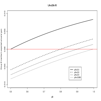
(a) 10 members in each group.

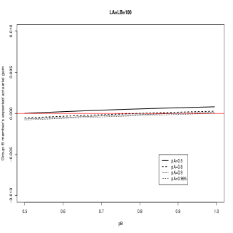
(b) 100 members in each group.

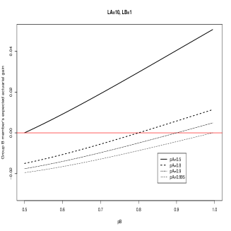
(c) 10 members in Group A, 1 member in Group B.

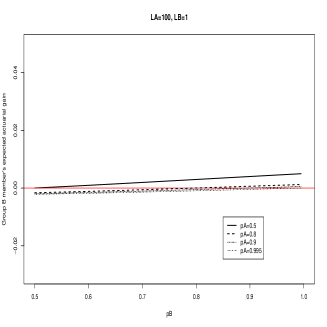
(d) 100 members in Group A, 1 member in Group B.

Figure 1: The expected actuarial gain per unit initial contribution for a Group $B$ member as the survival probability $p^{\textrm{B}}$ varies in a heterogeneous GSA. The figures show the gain for a fixed number of members in each group, fixed survival probabilities $p^{\textrm{A}}$ and the same initial contribution of 1 unit from each Group $A$ and Group $B$ member.

which is the expected actuarial gain from sharing mortality risk. In an actuarially fair fund, the net expected actuarial gain is zero for all members. If it is greater than zero for a member, then the member has an expected consumption that is higher than their initial contribution of 1 unit, and vice versa. The results, illustrated in Figure 1, show that

$$\mathbb{E}(c_{0}^{\textrm{B}}+c_{1}^{\textrm{B}})-1\left\{\begin{array}[]{ll}<0&\textrm{if $p^{\textrm{A}}>p^{\textrm{B}}$}\\ >0&\textrm{if $p^{\textrm{A}}<p^{\textrm{B}}$},\end{array}\right.$$

i.e. the GSA with different group survival probabilities is not actuarially fair.

4.4 Is actuarial unfairness financially significant?

We have shown that the GSA is actuarially unfair. Here we investigate if the fairness is financially significant. We find that it can be for small or highly heterogeneous groups. Qiao and Sherris (2013) analyze numerically the number of members required to adequately pool mortality risk in a heterogeneous GSA.

First we calculate Bob’s expected actuarial gain per unit initial contribution in a heterogeneous GSA, i.e.

$$\frac{\mathbb{E}(c_{0}^{\textrm{B}}+c_{1}^{\textrm{B}})-F^{\textrm{B}}_{0}}{F^{\textrm{B}}_{0}}$$

(in an actuarially-fair fund, the expected actuarial gain is zero for each member).

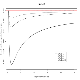
(a) 10 members in each group.

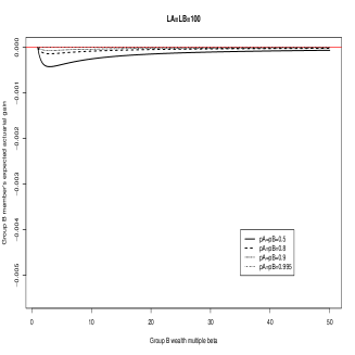
(b) 100 members in each group.

(c) 10 members in Group A, 1 member in Group B.

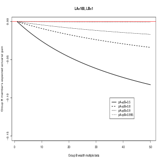
(d) 100 members in Group A, 1 member in Group B.

Figure 2: The expected actuarial gain per unit initial contribution for a Group B member as the initial contribution of the Group $B$ member varies, in a heterogeneous GSA. The figures show the gain for a fixed number of members in each group, fixed survival probabilities $p^{\textrm{A}}$ and $p^{\textrm{B}}$, and initial contribution of 1 unit from each Group $A$ member.

The expected actuarial gain is shown in Figures 1 and 2 for various sample heterogeneous GSAs. The results show that it is only with very small or highly heterogeneous groups that Bob’s expected actuarial loss is significant. For example, for $p^{\textrm{A}}=p^{\textrm{B}}=0.9$, Bob the only member of Group $B$ and Bob making 10 times the initial contribution of each Group $A$ member, Bob’s expected actuarial gain is $-2.4\%$ with 10 members in Group $A$, but this declines to $-0.4\%$ with 100 members in Group $A$.

Next we turn to Bob’s gain conditional upon his survival to time 1, relative to a homogeneous GSA in which everyone has the same probability of survival as Bob. If the conditional gains are greater than zero, then Bob can obtain a higher consumption while he is alive from the heterogeneous GSA, and vice versa.

Specifically, we calculate the excess of Bob’s expected conditional consumption

$$\mathbb{E}(c_{0}^{\textrm{B}}+c_{1}^{\textrm{B}}\,\big{|}\,\textrm{Bob survives to time 1})$$

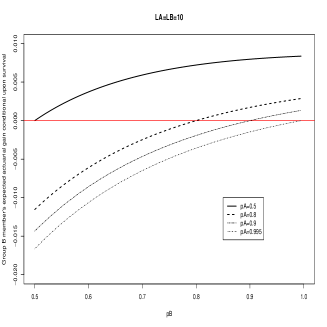
(a) 10 members in each group.

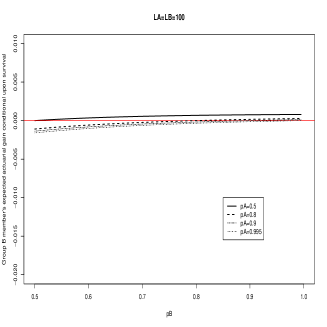
(b) 100 members in each group.

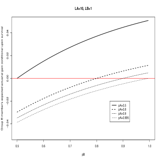
(c) 10 members in Group A, 1 member in Group B.

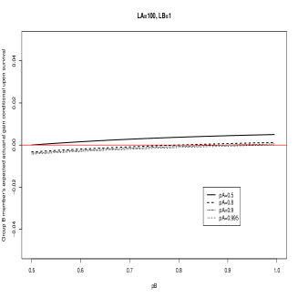
(d) 100 members in Group A, 1 member in Group B.

Figure 3: The relative expected actuarial gain, conditional upon survival to time 1, per unit initial contribution for a Group $B$ member as the survival probability $p^{\textrm{B}}$ varies, in a heterogeneous GSA. The figures show the gain for a fixed number of members in each group, fixed survival probabilities $p^{\textrm{A}}$ and the same initial contribution of 1 unit from each Group $A$ and Group $B$ member.

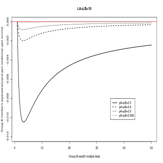
(a) 10 members in each group.

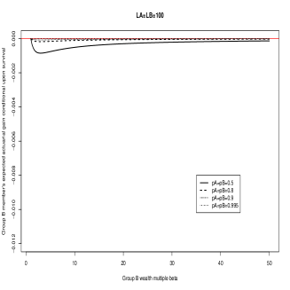
(b) 100 members in each group.

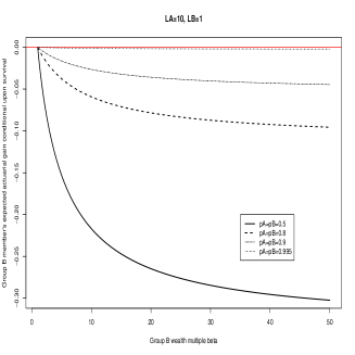
(c) 10 members in Group A, 1 member in Group B.

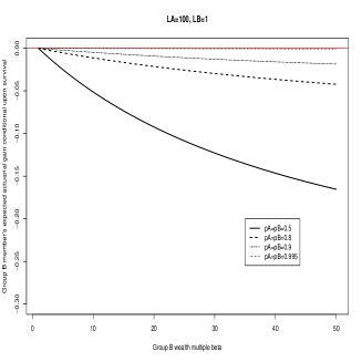
(d) 100 members in Group A, 1 member in Group B.

Figure 4: The relative expected actuarial gain, conditional upon survival to time 1, per unit initial contribution for a Group $B$ member as the initial contribution of the Group $B$ member varies, in a heterogeneous GSA. The figures show the gain for a fixed number of members in each group, fixed survival probabilities $p^{\textrm{A}}$ and $p^{\textrm{B}}$, and initial contribution of 1 unit from each Group $A$ member.

from a heterogeneous GSA over his expected conditional consumption from a homogeneous GSA, in which all members make the same initial contribution as Bob. This gives Bob’s relative expected actuarial gain conditional upon survival to time 1. We divide the relative conditional expected actuarial gain by Bob’s initial contribution. Figures 3 and 4 illustrate the results.

Again we see that it is only with small or highly heterogeneous groups that the relative conditional gain is significant. For example, for $p^{\textrm{A}}=p^{\textrm{B}}=0.9$, Bob the only member of Group $B$ and and Bob contributing 10 times the initial amount of each Group $A$ member, Bob’s expected conditional actuarial gain is $-2.6\%$ with 10 members in Group $A$, declining to $-0.5\%$ with 100 members in Group $A$.

4.5 Discussion of the GSA compared to a AOF for a heterogeneous group

A mortality risk-sharing arrangement does not create money for a group. It is simply a rule to allocate the group’s funds among the participants. However, the AOF and the GSA approach the sharing of mortality risk differently. They have different aims. In the GSA, the approach is a group risk-sharing perspective and in the AOF it is an individual member perspective.

The GSA assumes that the actual number of deaths in the scheme should be the expected number of deaths, assuming no longevity risk, since this is the basis of the calculation of the future consumption payments. This is reasonable when there are enough members to sufficiently pool mortality risk, by the Law of Large Numbers. In the GSA, deviations of the observed number of deaths from the expected number of deaths result in adjustments to the consumption payments. For example, if deaths turn out exactly as expected for Group $A$ but not as expected for Group $B$, then both Group $A$ and $B$ members will have their consumption payments adjusted by the same percentage.

The AOF starts with the requirement that the fund is actuarially fair for each member, by taking into account the actual scheme membership profile in the calculation of the actuarial gains due to mortality risk-sharing. Actuarial gains due to deaths in the AOF result in members’ fund values changing by different percentages, according to their individual mortality rate and wealth, rather than by the same percentage as in the GSA.

The structure of the GSA is focused on paying its members a consumption stream. Members pay an initial contribution and do not individually own a share of the assets of the GSA. This means that individuals give up their claim on their initial contribution in exchange for the consumption stream.

In contrast, the AOF emphasizes an investment frame, in which the result of mortality risk-sharing is an additional, nonnegative return on an individual’s assets. Participants in an AOF retain investment control over their own assets. Indeed, theoretically these assets could include the individual’s house which would only need to be sold upon the death of the individual to order to share its financial value among the AOF members; in the meantime the individual could continue living in their house. This is unlike the GSA which, as it pays an income stream to its members, could not have its participants continuing to own and live in their own houses. The GSA requires the initial contributions upfront, whereas the AOF requires it upon the death of the member.

As the mortality risk-sharing rule in the AOF results in a payment to the estate of the recently deceased, there is less money to be shared among the survivors. Thus we expect that the survivors in an GSA should, considered as a group, gain more money than the survivors in the AOF no matter which future state of the world occurs.

However, this does not hold when we consider each survivor individually in a GSA. Consider the notional fund values in a GSA. Since

$$F^{\textrm{X}}_{0+}=F^{\textrm{X}}_{0}-c_{0}^{\textrm{X}}=p^{\textrm{X}}c_{0}^{\textrm{X}},$$

we find

$$F^{\textrm{X}}_{1}=\textrm{MEA}\cdot c_{0}^{\textrm{X}}=\textrm{MEA}\cdot\frac{F^{\textrm{X}}_{0+}}{p^{\textrm{X}}},$$

which implies

$$F^{\textrm{X}}_{1}\left\{\begin{array}[]{ll}>F^{\textrm{X}}_{0+}&\textrm{if $\textrm{MEA}>p^{\textrm{X}}$}\\ =F^{\textrm{X}}_{0+}&\textrm{if $\textrm{MEA}=p^{\textrm{X}}$}\\ <F^{\textrm{X}}_{0+}&\textrm{if $\textrm{MEA}<p^{\textrm{X}}$},\end{array}\right.$$

for $X\in\{A,B\}$. Hence it is possible that the notional fund value of a survivor in Group $A$ increases at time 1 while the notional fund value of a survivor in Group $B$ decreases at time 1. For example, consider a GSA with group wealth-mortality characteristics

$$\mathbf{z}^{A}=(L,p^{\textrm{A}},1)\quad\textrm{and}\quad\mathbf{z}^{B}=(L,p^{\textrm{B}},1),$$

with $p^{\textrm{B}}>p^{\textrm{A}}$. Then on the event $[N^{A}=N^{B}=0]$, the mortality experience adjustment factor defined by equation (4) becomes

$$\textrm{MEA}=\frac{2p^{\textrm{A}}p^{\textrm{B}}}{p^{\textrm{A}}+p^{\textrm{B}}}.$$

As $p^{\textrm{B}}>p^{\textrm{A}}$, it is straightforward to show that

$$\textrm{MEA}>p^{\textrm{A}}\qquad\textrm{and}\qquad\textrm{MEA}<p^{\textrm{B}}.$$

Thus with strictly positive probability,

$$F^{\textrm{A}}_{1}>F^{\textrm{A}}_{0+}\qquad\textrm{and}\qquad F^{\textrm{B}}_{1}<F^{\textrm{B}}_{0+},\qquad\textrm{on $[N^{A}=N^{B}=0]$}.$$

The interpretation is that when no-one in each group dies, the survivors in Group $B$ lose financially from pooling mortality in the GSA. In comparison, survivors in either group in the corresponding heterogeneous AOF never lose financially from pooling mortality (see Donnelly et al. 2013). In the heterogeneous AOF when no-one dies in either group by time 1, the fund values at time 1 of each member would equal their fund values at time 0 (ignoring investment returns).

Both structures mean that longevity risk is shared among the group. We have not analyzed the impact of longevity risk here, but instead refer the reader to Qiao and Sherris (2013) for the GSA. A related paper is Hanewald et al. (2013).

In conclusion, the attractiveness of the GSA over the AOF depends on an individual’s circumstances. One person may prefer to have an income stream paid from the GSA without having the worry of managing their own assets, another may prefer the flexibility of the AOF. We simply highlight that the structures are different in how they share mortality risk and that this has implications, both financial and for which assets can be used for the pooling.

5 Summary

Various risk-sharing pension schemes have been proposed in the literature, which do not involve a sponsoring employer or insurance company. We have highlighted the connections and differences between some of these schemes.

We have also examined if the group self-annuitization scheme is actuarially fair, and we have found that it is not fair for a finite, heterogeneous group. The primary reason for this result is that the Law of Large Numbers can only be approximately true for a finite group, while the calculation of the consumption payments in the group self-annuitization scheme assumes that mortality risk is fully diversified. The greater the heterogeneity in the fund, the greater is the number of members required to make the assumption of full diversification of mortality risk a reasonable approximation. Consequently, certain classes of members may be financially disadvantaged in a group self-annuitization scheme. While it may have been the intention of the authors who proposed the group self-annuitization scheme that they are only operated for large numbers of people, this is not often clearly stated.

The relative attractiveness of the examined schemes for different types of individuals is an important question that we leave for future work.

Appendix A Proofs

*

Proof.

In a heterogeneous GSA in which the wealth-mortality characteristics of

• Group $A$ are $\mathbf{z}^{A}=(L,p,1)$, i.e. $F^{\textrm{A}}_{0}=1$, and

• Group $B$ are $\mathbf{z}^{B}=(L,p,\beta)$, i.e. $F^{\textrm{B}}_{0}=\beta$,

denote by

• $c_{0}^{\textrm{B}}(\beta)$ the consumption at time 0 of a member of Group $B$,

• $c_{1}^{\textrm{B}}(\beta)$ the consumption at time 1 of a surviving member of Group $B$,

• $f(\beta):=\mathbb{E}(c_{0}^{\textrm{B}}(\beta)+c_{1}^{\textrm{B}}(\beta)\,\big{|}\,\textrm{Bob survives to time 1})$ the expected consumption of Bob conditional upon his survival to time 1, and

• $g(\beta):=\mathbb{E}(c_{0}^{\textrm{B}}(\beta)+c_{1}^{\textrm{B}}(\beta))$ the expected consumption of Bob.

We begin by showing that, conditional upon his survival to time 1, Bob’s expected consumption in the heterogeneous GSA is different than in a homogeneous GSA, in which all surviving members have the same amount of wealth as Bob. Specifically, we prove that

$$f(\beta)\left\{\begin{array}[]{ll}<\beta f(1)&\textrm{if $\beta>1$}\\ =\beta f(1)&\textrm{if $\beta=1$}\\ >\beta f(1)&\textrm{if $\beta<1$},\end{array}\right.$$ (7)

in which $\beta f(1)$ is Bob’s conditional expected consumption in a homogeneous GSA in which all members make the same initial contribution $\beta$.

From (3),

$$F^{\textrm{X}}_{0+}:=F^{\textrm{X}}_{0}-c_{0}^{\textrm{X}}=F^{\textrm{X}}_{0}\left(1-\frac{1}{\ddot{a}_{0}^{X}}\right)=F^{\textrm{X}}_{0}\frac{p}{1+p},$$

so that from (4) and (5) we find

$$\begin{split}\mathbb{E}(c_{1}^{\textrm{B}}(\beta)\,|\,\textrm{Bob survives to time 1})=&\mathbb{E}(c_{0}^{\textrm{X}}\cdot\textrm{MEA}\,|\,\textrm{Bob survives to time 1})\\ =&\mathbb{E}\left(\frac{\beta}{1+p}\cdot\frac{p(\beta+1)L}{L-N^{A}+\beta(L-N^{B})}\,\bigg{|}\,\textrm{Bob survives to time 1}\right).\end{split}$$

Set $q:=1-p$. Since $N^{A}\sim BIN(L,q)$ and $N^{B}\sim BIN(L-1,q)$, we get

$$f(\beta)=\frac{\beta}{1+p}+\frac{p}{1+p}\sum_{n=0}^{L}\sum_{m=0}^{L-1}\frac{\beta(\beta+1)}{L-n+\beta(L-m)}\,\binom{L}{n}\binom{L-1}{m}q^{n+m}p^{2L-1-(n+m)}.$$

Define

$$h(n,m,\beta):=\frac{\beta(\beta+1)}{L-n+\beta(L-m)}\,\binom{L}{n}\binom{L-1}{m}q^{n+m}p^{2L-1-(n+m)},$$

which allows us to write more compactly

$$\begin{split}f(\beta)&=\frac{\beta}{1+p}+\frac{p}{1+p}\sum_{n=0}^{L}\sum_{m=0}^{L-1}h(n,m,\beta)\\ &=\frac{\beta}{1+p}+\frac{p}{1+p}\sum_{n=0}^{L-1}\sum_{m=0}^{L-1}h(n,m,\beta)+\frac{p}{1+p}\sum_{m=0}^{L-1}h(L,m,\beta).\end{split}$$

First, as

$$\sum_{n=0}^{L-1}\sum_{m=0}^{L-1}h(n,m,\beta)=\sum_{n=0}^{L-1}h(n,n,\beta)+\mathds{1}_{\left[L\geq 2\right]}\sum_{n=0}^{L-2}\sum_{m=n+1}^{L-1}\left[h(n,m,\beta)+h(m,n,\beta)\right]$$

and

$$\sum_{m=0}^{L-1}h(L,m,\beta)=(\beta+1)\frac{q^{L}(1-q^{L})}{p},$$

then

$$\begin{split}f(\beta)&=\frac{\beta}{1+p}+\frac{p}{1+p}\left(\sum_{n=0}^{L-1}h(n,n,\beta)+\mathds{1}_{\left[L\geq 2\right]}\sum_{n=0}^{L-2}\sum_{m=n+1}^{L-1}\left[h(n,m,\beta)+h(m,n,\beta)\right]\right)\\ &+\frac{(\beta+1)q^{L}(1-q^{L})}{1+p}.\end{split}$$

Thus

$$\begin{split}\beta f(1)-f(\beta)&=\frac{p}{1+p}\sum_{n=0}^{L-1}\left[\beta h\left(n,n,1\right)-h(n,n,\beta)\right]\\ &+\mathds{1}_{\left[L\geq 2\right]}\frac{p}{1+p}\sum_{n=0}^{L-2}\sum_{m=n+1}^{L-1}\left(\beta\left[h(n,m,1)+h(m,n,1)\right]-\left[h(n,m,\beta)+h(m,n,\beta)\right]\right)\\ &+\frac{(\beta-1)q^{L}(1-q^{L})}{1+p}.\end{split}$$ (8)

Next, after some algebra, we find for $n=0,1,\ldots,L-1$ that

$$h\left(n,n,\beta\right)=\beta\,h\left(n,n,1\right)$$

and

$$\begin{split}&h(n,m,\beta)+h(n,m,\beta)\\ =&\frac{\beta(\beta+1)}{L}\binom{L}{n}\binom{L}{m}q^{n+m}p^{2L-1-(n+m)}\left[\frac{L-m}{L-n+\beta(L-m)}+\frac{L-n}{L-m+\beta(L-n)}\right],\end{split}$$

which allows us to simplify equation (8) to

$$\begin{split}&\beta f(1)-f(\beta)\\ =&\frac{\beta-1}{1+p}\\ &\cdot\left[\frac{\beta p}{L}\mathds{1}_{\left[L\geq 2\right]}\sum_{n=0}^{L-2}\sum_{m=n+1}^{L-1}\binom{L}{n}\binom{L}{m}\frac{(n-m)^{2}q^{n+m}p^{2L-1-(n+m)}}{\left[L-n+\beta(L-m)\right]\left[L-m+\beta(L-n)\right]}+q^{L}(1-q^{L})\right].\end{split}$$

From the positivity of the terms in the square bracket we obtain the required inequality (7).

Now turning to Bob’s expected consumption, we show that his expected consumption in the heterogeneous GSA is different than in a homogeneous GSA, in which all surviving members have the same amount of wealth as Bob. Recall that his expected consumption is given by

$$g(\beta)=\mathbb{E}(c_{0}^{\textrm{B}}(\beta)+c_{1}^{\textrm{B}}(\beta)).$$

We prove that

$$g(\beta)\left\{\begin{array}[]{ll}<\beta&\textrm{if $\beta>1$}\\ =\beta&\textrm{if $\beta=1$}\\ >\beta&\textrm{if $\beta<1$}.\end{array}\right.$$ (9)

We assume that if everyone in the GSA dies by time 1 then the estates of the members receive their individual notional fund values. Then

$$\begin{split}g(\beta)&=pf(\beta)+q\mathbb{E}(c_{0}^{\textrm{B}}(\beta)+c_{1}^{\textrm{B}}(\beta)\,|\,\textrm{Bob dies by time 1})\\ &=pf(\beta)+q\left(\frac{\beta}{1+p}+\frac{\beta p}{1+p}q^{2L-1}\right),\end{split}$$

from which we obtain

$$\beta g(1)-g(\beta)=p\left(\beta f(1)-f(\beta)\right).$$

Upon noting that the homogeneous GSA is actuarially fair, i.e. $g(1)=1$, and that $p\in(0,1)$, the inequality (9) follows from (7). ∎

*

Proof.

In a heterogeneous GSA in which the wealth-mortality characteristics of

• Group $A$ are $\mathbf{z}^{A}=(L^{A},p,1)$, i.e. $F^{\textrm{A}}_{0}=1$, and

• Group $B$ are $\mathbf{z}^{B}=(1,p,\beta)$, i.e. $F^{\textrm{B}}_{0}=\beta$,

denote by

• $c_{0}^{\textrm{B}}(\beta)$ the consumption at time 0 of Bob,

• $c_{1}^{\textrm{B}}(\beta)$ the consumption at time 1 of Bob if he survives to time 1,

• $f(\beta):=\mathbb{E}(c_{0}^{\textrm{B}}(\beta)+c_{1}^{\textrm{B}}(\beta)\,\big{|}\,\textrm{Bob survives to time 1})$ the expected consumption of Bob conditional upon his survival to time 1, and

• $g(\beta):=\mathbb{E}(c_{0}^{\textrm{B}}(\beta)+c_{1}^{\textrm{B}}(\beta))$ the expected consumption of Bob.

We begin by showing that, conditional upon his survival to time 1, Bob’s expected consumption in the heterogeneous GSA is different than in a homogeneous GSA, in which all surviving members have the same amount of wealth as Bob. As before, we show that

$$f(\beta)\left\{\begin{array}[]{ll}<\beta f(1)&\textrm{if $\beta>1$}\\ =\beta f(1)&\textrm{if $\beta=1$}\\ >\beta f(1)&\textrm{if $\beta<1$}.\end{array}\right.$$ (10)

From (4) and (5),

$$\begin{split}&\mathbb{E}(c_{1}^{\textrm{B}}(\beta)\,|\,\textrm{Bob survives to time 1})\\ =&\mathbb{E}\left(\frac{\beta}{1+p}\cdot\frac{p\left(L+\beta\right)}{L-N^{A}+\beta}\,\bigg{|}\,\textrm{Bob survives to time 1}\right).\end{split}$$

Set $q:=1-p$. Since $N^{A}\sim BIN(L,q)$, we get

$$f(\beta)=\frac{\beta}{1+p}+\frac{p}{1+p}\sum_{n=0}^{L}\frac{\beta(L+\beta)}{L+\beta-n}\,\binom{L}{n}q^{n}p^{L-n}.$$

Thus

$$\begin{split}\beta f(1)-f(\beta)&=\frac{\beta p}{1+p}\sum_{n=0}^{L}\binom{L}{n}q^{n}p^{L-n}\left[\frac{L+1}{L+1-n}-\frac{L+\beta}{L+\beta-n}\right]\\ &=\frac{\beta(\beta-1)p}{1+p}\sum_{n=0}^{L}\binom{L}{n}q^{n}p^{L-n}\frac{n}{(L+1-n)(L+\beta-n)},\end{split}$$

so that the sign of $\beta f(1)-f(\beta)$ is inherited from the sign of $\beta-1$. Thus we obtain the inequality (10).

Now turning to Bob’s overall expected consumption, the proof that

$$g(\beta)\left\{\begin{array}[]{ll}<\beta&\textrm{if $\beta>1$}\\ =\beta&\textrm{if $\beta=1$}\\ >\beta&\textrm{if $\beta<1$}\end{array}\right.$$

is identical to that in Proposition 4.3. ∎

Appendix B Figures

References

- Donnelly (2014) C. Donnelly. Quantifying mortality risk in small defined-benefit pension schemes. Scandinavian Actuarial Journal, 2014(1):41–57, 2014.
- Donnelly et al. (2013) C. Donnelly, M. Guillén, and J.P. Nielsen. Exchanging uncertain mortality for a cost. Insurance: Mathematics and Economics, 52(1):65–76, 2013.
- Donnelly et al. (2014) C. Donnelly, M. Guillén, and J.P. Nielsen. Bringing cost transparency to the life annuity market. Insurance: Mathematics and Economics, 56:14–27, 2014.
- Hanewald et al. (2013) K. Hanewald, J. Piggott, and M. Sherris. Individual post-retirement longevity risk management under systematic mortality risk. Insurance: Mathematics and Economics, 52(1):87–97, 2013.
- Piggott et al. (2005) J. Piggott, E.A. Valdez, and B. Detzel. The simple analytics of a pooled annuity fund. Journal of Risk and Insurance, 72(3):497–520, 2005.
- Pension Protection Fund (2013) PPF. The purple book: DB pensions universe risk profile, 2013. Produced by the Pension Protection Fund and The Pensions Regulator. Published on 5 November 2013. http://www.pensionprotectionfund.org.uk/Pages/ThePurpleBook.aspx.
- Qiao and Sherris (2013) C. Qiao and M. Sherris. Managing systematic mortality risk with group self pooling and annuitization schemes. Journal of Risk and Insurance, 80(4):949––974, 2013.
- Sabin (2010) M.J. Sabin. Fair tontine annuity. http://ssrn.com/abstract=1579932, March 2010.
- Stamos (2008) M.Z. Stamos. Optimal consumption and portfolio choice for pooled annuity funds. Insurance: Mathematics and Economics, 43(1):56–68, 2008.