Non-Kähler Expanding Ricci Solitons II

Abstract.

We produce new non-Kähler, non-Einstein, complete expanding gradient Ricci solitons with conical asymptotics and underlying manifold of the form $\mbox{${\mathbb{R}}$}^{2}\times M_{2}\times\cdots\times M_{r}$, where $r\geq 2$ and $M_{i}$ are arbitrary closed Einstein spaces with positive scalar curvature. We also find numerical evidence for complete expanding solitons on the vector bundles whose sphere bundles are the twistor or ${\rm Sp}(1)$ bundles over quaternionic projective space.

Mathematics Subject Classification (2000): 53C25, 53C44

0. Introduction

In [BDGW] we constructed complete steady gradient Ricci soliton structures (including Ricci-flat metrics) on manifolds of the form ${\mbox{${\mathbb{R}}$}}^{2}\times M_{2}\times\ldots\times M_{r}$ where $M_{i},\,2\leq i\leq r,$ are arbitrary closed Einstein manifolds with positive scalar curvature. We also produced numerical solutions of the steady gradient Ricci soliton equation on certain non-trivial $\mbox{${\mathbb{R}}$}^{3}$ and $\mbox{${\mathbb{R}}$}^{4}$ bundles over quaternionic projective spaces. In the current paper we will present the analogous results for the case of expanding solitons on the same underlying manifolds.

Recall that a gradient Ricci soliton is a manifold $M$ together with a smooth Riemannian metric $g$ and a smooth function $u$, called the soliton potential, which give a solution to the equation:

(0.1) $${{\rm Ric}}(g)+{\rm Hess}(u)+\frac{\epsilon}{2}\,g=0$$

for some constant $\epsilon$. The soliton is then called expanding, steady, or shrinking according to whether $\epsilon$ is greater, equal, or less than zero.

A gradient Ricci soliton is called complete if the metric $g$ is complete. The completeness of the vector field $\nabla u$ follows from that of the metric (cf [Zh]). If the metric of a gradient Ricci soliton is Einstein, then either ${\rm Hess}\,u=0$ (i.e., $\nabla u$ is parallel) or we are in the case of the Gaussian soliton (cf [PW] or [PRS]).

At present most examples of non-Kählerian expanding solitons arise from left-invariant metrics on nilpotent and solvable Lie groups (resp. nilsolitons, solvsolitons), as a result of work by J. Lauret [La1], [La3], M. Jablonski [Ja], and many others (cf the survey [La2]). These expanders are however not of gradient type, i.e., they satisfy the more general equation

(0.2) $${{\rm Ric}}(g)+\frac{1}{2}\,{\sf L}_{X}g+\frac{\epsilon}{2}\,g=0$$

where $X$ is a vector field on $M$ and ${\sf L}$ denotes Lie differentiation.

A large class of complete, non-Einstein, non-Kählerian expanders of gradient type (with dimension $\geq 3$) consists of an $r$-parameter family of solutions to (0.1) on $\mbox{${\mathbb{R}}$}^{k+1}\times M_{2}\times\ldots\times M_{r}$ where $k>1$ and $M_{i}$ are positive Einstein manifolds. The special case $r=1$ (i.e., no $M_{i}$) is due to Bryant [Bry] and the solitons have positive sectional curvature. The $r=2$ case is due to Gastel and Kronz [GK], who adapted Böhm’s construction of complete Einstein metrics with negative scalar curvature to the soliton case. The case of arbitrary $r$ was treated in [DW3] via a generalization of the dynamical system studied by Bryant. The soliton metrics in this family are all of multiple warped product type. In other words, the manifold is thought of as being foliated by hypersurfaces of the form $S^{k}\times M_{2}\times\ldots\times M_{r}$ each equipped with a product metric depending smoothly on a real parameter $t$.

More recently, Schulze and Simon [SS] constructed expanding gradient Ricci solitons with non-negative curvature operator in arbitrary dimensions by studying the scaling limits of the Ricci flow on complete open Riemannian manifolds with non-negative bounded curvature operator and positive asymptotic volume ratio.

As pointed out in [BDGW], the situation of multiple warped products on nonnegative Einstein manifolds is rather special because of the automatic lower bound on the scalar curvature of the hypersurfaces. This leads, in the case where all factors have positive scalar curvature, i.e., $k>1$, to definiteness of certain energy functionals occurring in the analysis of the dynamical system arising from (0.1), and hence to coercive estimates on the flow. In the present case, where one factor is a circle, i.e., $k=1$, we can pass, as in [BDGW], to a subsystem where coercivity holds, and this is enough for the analysis to proceed. The new solitons obtained, like those of [DW3], have conical asymptotics, and are not of Kähler type (Theorem 2.14). We note that the lowest dimensional solitons we obtain form a $2$-parameter family on $\mbox{${\mathbb{R}}$}^{2}\times S^{2}$. The special case $r=1$ was analysed earlier by the physicists Gutperle, Headrick, Minwalla and Schomerus [GHMS].

As in [BDGW] we also obtain a family of solutions to our soliton equations that yield complete Einstein metrics of negative scalar curvature (Theorem 3.1). These are analogous to the metrics discovered by Böhm in [Bo]. Recall that for Böhm’s construction the fact that the hyperbolic cone over the product Einstein metric on the hypersurface acts as an attractor plays an important role in the convergence proof for the Einstein trajectories. When $k=1$, however, no product metric on the hypersurface can be Einstein with positive scalar curvature, so the hyperbolic cone construction cannot be exploited directly. It turns out that the analysis of the soliton case already contains most of the analysis required for the Einstein case. The new Einstein metrics we obtain have exponential volume growth.

Since the underlying smooth manifolds in the present paper are identical to those in [BDGW], our constructions give rise to pairs of homeomorphic but not diffeomorphic non-Einstein expanding gradient Ricci solitons as well as similar pairs of complete Einstein manifolds with negative scalar curvature. Furthermore, since our expanders and Einstein metrics have asymptotically conical structures, we also obtain pairs whose asymptotic cones are homeomorphic but not diffeomorphic. The details can be found at the end of §3.

To make further progress in the search for expanders, we need to consider more complicated hypersurface types where the scalar curvature may not be bounded below. In [BDGW] we carried out numerical investigations of steady solitons where the hypersurfaces are the total spaces of Riemannian submersions for which the hypersurface metric involves two functions, one scaling the base and one the fibre of the submersion. We now look numerically at expanding solitons with such hypersurface types, in particular where the hypersurfaces are $S^{2}$ or $S^{3}$ bundles over quaternionic projective space. We produce numerical evidence of complete expanding gradient Ricci soliton structures in these cases.

Before undertaking our theoretical and numerical investigations, we first prove some general results about expanding solitons of cohomogeneity one type. Some of the results follow from properties of general expanding gradient Ricci solitons. However, the proofs are much simpler and sometimes the statements are sharper, which is helpful in numerical studies. The results include monotonicity and concavity properties for the soliton potential similar to those proved in [BDGW] in the steady case, as well as an upper bound for the mean curvature of the hypersurfaces. To derive this bound, we need to know that complete non-Einstein expanding gradient Ricci solitons have infinite volume. We include a proof of this fact here (Prop. 1.22) since we were not able to find an explicit statement in the literature. Finally we derive an asymptotic lower bound for the gradient of the soliton potential, which is in turn used to exhibit a general Lyapunov function for the cohomogeneity one expander equations.

1. Background on cohomogeneity one expanding solitons

We briefly review the formalism [DW1] for Ricci solitons of cohomogeneity one. We work on a manifold $M$ with an open dense set foliated by equidistant diffeomorphic hypersurfaces $P_{t}$ of real dimension $n$. The dimension of $M$, the manifold where we construct the soliton, is therefore $n+1$. The metric is then of the form $\bar{g}=dt^{2}+g_{t}$ where $g_{t}$ is a metric on $P_{t}$ and $t$ is the arclength coordinate along a geodesic orthogonal to the hypersurfaces. This set-up is more general than the cohomogeneity one ansatz, as it allows us to consider metrics with no symmetry provided that appropriate additional conditions on $P_{t}$ are satisfied, see the following as well as Remarks 2.18 and 3.18 in [DW1]. We will also suppose that $u$ is a function of $t$ only.

We let $r_{t}$ denote the Ricci endomorphism of $g_{t}$, defined by ${\rm Ric}(g_{t})(X,Y)=g_{t}(r_{t}(X),Y)$ and viewed as an endomorphism via $g_{t}$. Also let $L_{t}$ be the shape operator of the hypersurfaces, defined by the equation $\dot{g_{t}}=2g_{t}L_{t}$ where $g_{t}$ is regarded as an endomorphism with respect to a fixed background metric $Q$. The Levi-Civita connections of $\bar{g}$ and $g_{t}$ will be denoted by $\overline{\nabla}$ and $\nabla$ respectively. The relative volume $v(t)$ is defined by $d\mu_{g_{t}}=v(t)\,d\mu_{Q}$

We assume that the scalar curvature $S_{t}={\rm tr}(r_{t})$ and the mean curvature ${\rm tr}(L_{t})$ (with respect to the normal $\nu=\frac{\partial}{\partial t}$) are constant on each hypersurface. These assumptions hold, for example, if $M$ is of cohomogeneity one with respect to an isometric Lie group action. They are satisfied also when $M$ is a multiple warped product over an interval.

The gradient Ricci soliton equation now becomes the system

(1.1) $$-{\rm tr}(\dot{L})-{\rm tr}(L^{2})+\ddot{u}+\frac{\epsilon}{2} = 0,$$

(1.2) $$r-({\rm tr}\,L)L-\dot{L}+\dot{u}L+\frac{\epsilon}{2}\,\mbox{${\mathbb{I}}$} = 0,$$

(1.3) $$d({\rm tr}L)+\delta^{\nabla}L = 0.$$

The first two equations represent the components of the equation in the directions normal and tangent to the hypersurfaces $P$, respectively. The third equation represents the equation in mixed directions—here $\delta^{\nabla}L$ denotes the codifferential for $TP$-valued $1$-forms.

In the warped product case the final equation involving the codifferential automatically holds. This is also true for cohomogeneity one metrics that are monotypic, i.e., when there are no repeated real irreducible summands in the isotropy representation of the principal orbits (cf [BB], Prop. 3.18).

There is a conservation law

(1.4) $$\ddot{u}+(-\dot{u}+{\rm tr}\,L)\,\dot{u}-\epsilon u=C$$

for some constant $C$. Using our equations we may rewrite this as

(1.5) $$S+{\rm tr}(L^{2})-(\dot{u}-{\rm tr}\,L)^{2}-\epsilon u+\frac{1}{2}(n-1)\epsilon=C.$$

where $S:={\rm tr}(r_{t})$ is the scalar curvature $S$ of the principal orbits. If $\bar{R}$ denotes the scalar curvature of the ambient metric $\bar{g}$, then

$$\bar{R}=-2{\rm tr}(\dot{L})-{\rm tr}(L^{2})-({\rm tr}L)^{2}+S.$$

We can deduce the equality

(1.6) $$\bar{R}+\dot{u}^{2}+\epsilon u=-C-\frac{\epsilon}{2}(n+1).$$

We let $\xi$ denote the dilaton mean curvature

$$\xi:=-\dot{u}+{\rm tr}\,L.$$

This is the mean curvature of the dilaton volume element $e^{-u}d\mu_{\bar{g}}$. It is often useful to define a new independent variable $s$ by

(1.7) $$\frac{d}{ds}:=\frac{1}{\xi}\frac{d}{dt},$$

and use a prime to denote $\frac{d}{ds}$. We note that equation (1.1) implies that $\dot{\xi}=-{\rm tr}(L^{2})+\frac{\epsilon}{2}$.

It is also useful, following [DHW], to introduce the quantity

$$\mbox{${\mathcal{E}}$}:=C+\epsilon u.$$

The conservation law may now be rewritten (for nonzero $\epsilon$) as

(1.8) $$\ddot{\mbox{${\mathcal{E}}$}}+\xi\dot{\mbox{${\mathcal{E}}$}}-\epsilon\mbox{${\mathcal{E}}$}=0.$$

Note that for a function $t\mapsto f(t)$, the quantity $\ddot{f}+\xi\dot{f}$ is just the $u$-Laplacian in the sense of metric measure spaces.

Another useful quantity is the normalised mean curvature

$${\mathcal{H}}=\frac{{\rm tr}L}{\xi}=1+\frac{\dot{u}}{\xi}=1+u^{\prime},$$

which was introduced in [DW3] and [DHW].

We now specialise to the case of expanding solitons, that is

$$\epsilon>0.$$

We shall consider complete noncompact expanding solitons with one special orbit. We may take the interval $I$ over which $t$ ranges to be $[0,\infty)$ with the special orbit placed at $t=0$. Let $k$ denote the dimension of the collapsing sphere at $t=0$. We will moreover assume in this section that $u(0)=0$, since adding a constant to the soliton potential does not affect the equations.

A basic result of B.L. Chen [Chb] together with the strong maximum principle says that for a non-Einstein expanding gradient Ricci soliton $\bar{R}>-\frac{\epsilon}{2}(n+1)$. So we deduce from (1.6) that

$$\mbox{${\mathcal{E}}$}<0\,\,\,\,\mbox{and}\,\,\,\,(\dot{u})^{2}<-\mbox{${\mathcal{E}}$}:=-(C+\epsilon u).$$

Using the first inequality and the smoothness conditions at $t=0$ we find as in the steady case that $\ddot{u}(0)=\frac{C}{k+1}<0$, so completeness imposes restrictions on our initial conditions.

Integrating the second inequality and using the initial conditions yield

(1.9) $$0\leq-u(t)<\frac{\epsilon}{4}t^{2}+\sqrt{-C}t$$

and

(1.10) $$|\dot{u}|<\frac{\epsilon}{2}t+\sqrt{-C}.$$

These are just the cohomogeneity one versions of general estimates of the potential due to Z.-H. Zhang [Zh].

Proposition 1.11.

For a non-Einstein, complete, expanding gradient Ricci soliton of cohomogeneity one with a special orbit, the soliton potential $u$ is strictly decreasing and strictly concave on $(0,\infty)$.

Proof.

The conservation law (1.8) and the fact that ${\mathcal{E}}$ is negative and $\epsilon$ is positive show that $u$ is strictly concave on a neighbourhood of each critical point $t_{0}$. As we noted above, we also have concavity at the special orbit $t=0$. Now, as in the steady case [BDGW], we see there are no critical points of $u$ in $(0,\infty)$. As $\dot{u}(0)=0$, we see $u$ is strictly decreasing on $(0,\infty)$.

Now set $y=\dot{u}$ and differentiate (1.4); using (1.1) we obtain

$$\ddot{y}+\xi\dot{y}-\left(\frac{\epsilon}{2}+{\rm tr}(L^{2})\right)y=0.$$

In particular $\ddot{y}+\xi\dot{y}<0$ since $y$ is negative. Integrating shows $ve^{-u}\dot{y}$ is strictly decreasing, where we recall that $v$ is the relative volume. As $t$ tends to $0$, the smoothness conditions imply that $ve^{-u}\dot{y}$ tends to zero, so $\dot{y}=\ddot{u}$ is negative, as required. ∎

Our next result is inspired by the work of Munteanu-Sesum [MS] for the case of steady solitons.

Proposition 1.12.

For a non-Einstein, complete, expanding gradient Ricci soliton of cohomogeneity one with a special orbit, the volume growth is at least logarithmic.

Proof.

Let $M_{t}=\pi^{-1}([0,t])$ where $\pi$ is the projection of $M$ onto the orbit space $I$. We consider the integral

$$f(t):=\int_{M_{t}}\left(\bar{R}+\frac{\epsilon}{2}(n+1)\right)\;d\mu_{\bar{g}}$$

As we are considering non-Einstein solitons the integrand is positive.

Let $t_{0}>0$ and let $b:=f(t_{0})$. Using the trace of the soliton equation and also the divergence theorem, we have, for $t\geq t_{0}$:

$$0<b\leq f(t) = -\int_{M_{t}}\bar{\triangle}u\;d\mu_{\bar{g}}$$

$$= \int_{\partial M_{t}}(\bar{\nabla}u)\cdot(-\frac{\partial}{\partial t})\,d\mu_{\bar{g}}|_{\partial M_{t}}$$

$$= |\dot{u}|\,v(t)$$

$$< (\frac{\epsilon}{2}t+\sqrt{-C})v(t)$$

where we use (1.10) in the last line. Hence $v(t)>\frac{b}{\frac{\epsilon}{2}t+\sqrt{-C}}$, and integrating yields

$${\rm vol}(M_{t})>{\rm vol}(M_{t_{0}})-\frac{2b}{\epsilon}\log(\frac{\epsilon}{2}t_{0}+\sqrt{-C})+\frac{2b}{\epsilon}\log(\frac{\epsilon}{2}t+\sqrt{-C}).$$

∎

Proposition 1.13.

Let $(M,\bar{g},u)$ be a non-Einstein, complete, expanding gradient Ricci soliton of cohomogeneity one with a special orbit. Then there exists $t_{1}>0$ such that on $(t_{1},\infty)$ we have ${\rm tr}\;L<\sqrt{\frac{n\epsilon}{2}}$.

Proof.

By Cauchy-Schwartz and the concavity result, we have

(1.14) $$\frac{d}{dt}({\rm tr}\;L)<\frac{\epsilon}{2}-{\rm tr}\;(L^{2})\leq\frac{\epsilon}{2}-\frac{1}{n}({\rm tr}\;L)^{2}.$$

Note that by the smoothness conditions ${\rm tr}\;L$ is strictly decreasing near $t=0$, and its limit as $t$ tends to zero from above is $+\infty$.

(i) First let us assume that $\frac{d}{dt}({\rm tr}L)$ is nonnegative at some $t_{1}$. The above inequality shows that $|{\rm tr}L|^{2}<\frac{\epsilon n}{2}$ at $t=t_{1}$.

Let us consider the solutions of the equation

(1.15) $$\dot{h}=\frac{\epsilon}{2}-\frac{1}{n}h^{2}.$$

These are the family of increasing functions

$$h(t)=\sqrt{\frac{\epsilon n}{2}}\left(\frac{a\exp(t\sqrt{\frac{2\epsilon}{n}})-1}{a\exp(t\sqrt{\frac{2\epsilon}{n}})+1}\right),$$

where $a$ is a positive constant, as well as the constant functions $\pm\sqrt{\frac{\epsilon n}{2}}$ which form the bounding envelope for this family. Hence ${\rm tr}\;L\leq h^{*}(t)<\sqrt{\frac{\epsilon n}{2}}$ where $h^{*}(t)$ is the solution to (1.15) which agrees with ${\rm tr}\;L$ at $t_{1}$.

(ii) Next suppose that $\frac{d}{dt}({\rm tr}L)$ is always negative. Now if ${\rm tr}L$ is ever zero then it is negative and bounded away from zero on some semi-infinite interval. Recalling that ${\rm tr}L=\frac{\dot{v}}{v}$ and integrating, we see that the soliton volume is finite, which contradicts Proposition 1.12. So ${\rm tr}L$ is positive on $(0,\infty)$, and, using Proposition 1.11, we see $\xi$ is also positive on this interval. Theorem 11 of [PRS] shows that $\xi$ tends to infinity as $t$ tends to $\infty$. But $\xi$ also tends to infinity as $t$ tends to zero, so we have a minimum $t_{1}$ where $\dot{\xi}$ vanishes. Now (1.1) shows ${\rm tr}(L^{2})=\frac{\epsilon}{2}$ at $t_{1}$ and Cauchy-Schwartz shows $({\rm tr}L)^{2}\leq\frac{n\epsilon}{2}$ at $t_{1}$. As ${\rm tr}L$ is decreasing, we have the desired result. ∎

Remark 1.16.

This bound on ${\rm tr}L$ is best possible, at least if we allow the solitons to be Einstein. Indeed, the negative scalar curvature Einstein metrics of Böhm [Bo] give exactly this bound, as ${\rm tr}L$ is asymptotic to $\frac{n\epsilon}{2}$.

Next we consider properties of the Lyapunov function ${\mathscr{F}}_{0}$ which was introduced by Böhm in [Bo] for the Einstein case and was subsequently studied in [DHW] and [BDGW] for the soliton case. Note that this function was denoted by $\mathscr{F}$ in [DHW].

Proposition 1.17.

Let ${\mathscr{F}}_{0}$ denote the function $v^{\frac{2}{n}}\left(S+{\rm tr}((L^{(0)})^{2})\right)$ defined on the velocity phase space of the cohomogeneity one expanding gradient Ricci soliton equations, with $L^{(0)}$ representing the trace-free part of $L$. Then along the trajectory of a complete smooth non-Einstein expanding soliton, ${\mathscr{F}}_{0}$ is non-increasing for sufficiently large $t$.

Proof.

The formula for $\frac{d}{dt}{\mathscr{F}}_{0}$ in Proposition 2.17 of [DHW] shows that the proposition would follow if for sufficiently large $t$ one can show that

$$\xi-\frac{1}{n}{\rm tr}\,L=-\dot{u}+\left(\frac{n-1}{n}\right)\,{\rm tr}\,L\geq 0.$$

We first note that ${\rm tr}\,L$ is eventually bounded below by $-\sqrt{\epsilon n/2}$. Otherwise at some $t=t_{1}>0$, ${\rm tr}\,L\leq-\sqrt{\epsilon n/2}$ and (1.14) shows that this inequality continues to hold from $t_{1}$ onwards. But this would imply that the soliton has finite volume, contradicting Proposition 1.12.

We are now done since the next proposition (part (i)) shows that $|\dot{u}|=-\dot{u}$ grows at least linearly for sufficiently large $t$. In particular, for large enough $t$, ${\mathcal{F}}_{0}$ fails to be strictly decreasing iff the shape operator of the hypersurfaces become diagonal. ∎

Proposition 1.18.

Let $(M,\bar{g},u)$ be a complete, non-Einstein, expanding gradient Ricci soliton of cohomogeneity one with a special orbit. Suppose $t_{1}>2\sqrt{\frac{5}{\epsilon}}$ and on $[t_{1},+\infty)$ we have an upper bound $\lambda_{0}>0$ for ${\rm tr}\,L$. Set $a:=\lambda_{0}+\sqrt{-C}$. Then on $[t_{1},+\infty)$ we have

• $|\overline{\nabla}u|=-\dot{u}(t)>\frac{9}{10}\left(\frac{-\dot{u}(t_{1})}{\frac{\epsilon}{2}t_{1}+a}\right)\left(\frac{\epsilon}{2}t+a\right)$,
  

• $\ddot{u}+\frac{\epsilon}{2}=-{\rm Ric}_{\bar{g}}(\frac{\partial}{\partial t},\frac{\partial}{\partial t})\leq\frac{\epsilon}{2}\left(1+\frac{9}{10}\frac{\dot{u}(t_{1})}{\frac{\epsilon}{2}t_{1}+a}\right).$

Proof.

By assumption and the upper bound (1.10) we have $\xi<\frac{\epsilon}{2}t+a$. Since $\dot{y}=\ddot{u}<0$ and $y=\dot{u}<0$ by Proposition 1.11, we see that $y$ satisfies the differential inequality

$$\ddot{y}+\left(\frac{\epsilon}{2}t+a\right)\,\dot{y}-\frac{\epsilon}{2}\,y<0.$$

We will now compare $y$ with solutions of the corresponding equation

(1.19) $$\ddot{x}+\left(\frac{\epsilon}{2}t+a\right)\,\dot{x}-\frac{\epsilon}{2}\,x=0,$$

which can be solved explicitly. This is because if we differentiate this equation, we obtain

$$\frac{d^{3}x}{dt^{3}}+\left(\frac{\epsilon}{2}t+a\right)\ddot{x}=0,$$

from which we can solve for $\ddot{x}$. Accordingly, upon integration and using (1.19) we obtain

(1.20) $$x(t)=-\left(\frac{\epsilon}{2}t+a\right)\left(\frac{c_{0}}{\frac{\epsilon}{2}t_{1}+a}-c_{1}e^{\frac{\epsilon}{4}t_{1}^{2}+at_{1}}\int_{t_{1}}^{t}\,\frac{e^{-\frac{\epsilon}{4}\tau^{2}-a\tau}}{(\frac{\epsilon}{2}\tau+a)^{2}}\,d\tau\right)$$

where $c_{0}$ and $c_{1}$ are arbitrary constants.

In order to apply Theorem 13 on p. 26 of [PrW], we must choose $x(t_{1})\geq y(t_{1})=\dot{u}(t_{1})$ and $\dot{x}(t_{1})\geq\dot{y}(t_{1})=\ddot{u}(t_{1})$. Since $x(t_{1})=-c_{0}$, we can maximize $c_{0}$ by choosing $x(t_{1})=\dot{u}(t_{1})$. It follows that

$$c_{1}=-\ddot{x}(t_{1})=-\frac{\epsilon}{2}\,x(t_{1})+\left(\frac{\epsilon}{2}t_{1}+a\right)\dot{x}(t_{1})\geq-\frac{\epsilon}{2}\,\dot{u}(t_{1})+\left(\frac{\epsilon}{2}t_{1}+a\right)\ddot{u}(t_{1}).$$

In particular, an admissible choice for $c_{1}$ is $c_{1}=\frac{\epsilon}{2}c_{0}>0$. With this choice, it remains to find an upper bound for the integral in (1.20).

To do this, we integrate by parts three times and then throw away the resulting term involving integration (this term is negative). Specifically, we have

$$\int_{\lambda_{1}}^{\lambda}\,\frac{e^{-\sigma^{2}/\epsilon}}{\sigma^{2}}\,d\sigma\leq\frac{\epsilon}{2}\left(\frac{e^{-\lambda_{1}^{2}/\epsilon}}{\lambda_{1}^{3}}\right)\left(1-\frac{3}{2}\frac{\epsilon}{\lambda_{1}^{2}}+\frac{15}{\lambda_{1}^{4}}\left(\frac{\epsilon}{2}\right)^{2}-\left(\frac{\lambda_{1}}{\lambda}\right)^{3}e^{-(\lambda^{2}-\lambda_{1}^{2})/\epsilon}\left(1-\frac{3}{2}\frac{\epsilon}{\lambda^{2}}+\frac{15}{\lambda^{4}}\left(\frac{\epsilon}{2}\right)^{2}\right)\right).$$

Using the change of independent variable $\lambda:=\frac{\epsilon}{2}t+a$ and the fact that

$$1-\frac{3\epsilon}{2}x+\frac{15}{4}\,\epsilon^{2}x^{2}=\left(1-\frac{3\epsilon}{4}\,x\right)^{2}+\frac{51}{16}\,\epsilon^{2}x^{2}\geq\frac{17}{20},$$

we obtain

$$e^{\frac{\epsilon}{4}t_{1}^{2}+at_{1}}\int_{t_{1}}^{t}\,\frac{e^{-\frac{\epsilon}{4}\tau^{2}-a\tau}}{(\frac{\epsilon}{2}\tau+a)^{2}}\,d\tau\leq$$

$$\hskip 28.45274pt\frac{1}{(\frac{\epsilon}{2}t_{1}+a)^{3}}\left(1-\frac{\epsilon}{2}\frac{3}{(\frac{\epsilon}{2}t_{1}+a)^{2}}+\left(\frac{\epsilon}{2}\right)^{2}\frac{15}{(\frac{\epsilon}{2}t_{1}+a)^{4}}-\frac{17}{20}\left(\frac{\frac{\epsilon}{2}t_{1}+a}{\frac{\epsilon}{2}t+a}\right)^{3}\frac{e^{\frac{\epsilon}{4}t_{1}^{2}+at_{1}}}{e^{\frac{\epsilon}{4}t^{2}+at}}\right).$$

If we substitute the above information together with the choice $c_{1}=\frac{\epsilon}{2}c_{0}$ in the comparison inequality $\dot{u}(t)\leq x(t)$ (for $t\geq t_{1}$), we obtain

$$-\dot{u}(t) \geq -\frac{\dot{u}(t_{1})}{\frac{\epsilon}{2}t_{1}+a}\left(\frac{\epsilon}{2}t+a\right)\left(1-\frac{\epsilon}{2}\frac{1}{(\frac{\epsilon}{2}t_{1}+a)^{2}}\left(1-\frac{\epsilon}{2}\frac{3}{(\frac{\epsilon}{2}t_{1}+a)^{2}}+\left(\frac{\epsilon}{2}\right)^{2}\frac{15}{(\frac{\epsilon}{2}t_{1}+a)^{4}}\right)\right)$$

$$\geq -\frac{\dot{u}(t_{1})}{\frac{\epsilon}{2}t_{1}+a}\left(\frac{\epsilon}{2}t+a\right)\left(1-\frac{\epsilon}{2}\frac{1}{(\frac{\epsilon}{2}t_{1}+a)^{2}}\right)$$

$$> \frac{9}{10}\left(-\frac{\dot{u}(t_{1})}{\frac{\epsilon}{2}t_{1}+a}\right)\left(\frac{\epsilon}{2}t+a\right)$$

where for the last inequality we used the hypothesis that $t_{1}>2\sqrt{\frac{5}{\epsilon}}$, so that $\frac{\epsilon}{2}t_{1}+a>\sqrt{5\epsilon}$. This completes the proof of (i).

The proof of (ii) follows by applying the same estimates to the comparison inequality $\ddot{u}(t)=\dot{y}(t)\leq\dot{x}(t)$ for $t\geq t_{1}$. Note that by (2.2) in [DW4] and (1.2), the quantity $\ddot{u}+\frac{\epsilon}{2}$ is precisely the negative of the Ricci curvature of the soliton metric in the direction $\frac{\partial}{\partial t}$. ∎

Remark 1.21.

In the above proof we can of course take $\lambda_{0}$ to be $\sqrt{\epsilon n/2}$ by Proposition 1.13. Notice, however, that in part (ii) of the proof of Proposition 1.13 one automatically has an upper bound on ${\rm tr}\,L$. So one can apply Proposition 1.18 instead of Theorem 11 of [PRS] to obtain a self-contained proof for Proposition 1.13.

Note also that both Propositions 1.13 and 1.18 do not require any curvature bounds.

We end this section with a simple generalization of Proposition 1.12 which, as far as we know, has not been explicitly observed in the literature. An analogous result for steady gradient Ricci solitons is Theorem 5.1 in [MS].

Proposition 1.22.

A complete non-Einstein expanding gradient Ricci soliton has at least logarithmic volume growth.

Proof.

The basic idea is the same as that for the cohomogeneity one case. Technically, we employ a formulation of the approximation arguments of Gaffney [Gaf] given by Yau in [Y] (p. 660) which provides a compact exhaustion of the underlying manifold with good properties for applying Stoke’s theorem.

Let $(M,g,u)$ denote our non-Einstein expander, which is necessarily non-compact. By going to the orientation double cover we may assume without loss of generality that $M$ is orientable. Let us fix a point $p\in M$ and denote by $r(x)$ the distance function from $p$, which is in general only Lipschitz continuous. Then for any value $r>0$, there exists a smooth positive function $\varphi_{r}$ on $M$ such that

1. except for finitely many $t<r$, $\varphi_{r}^{-1}(t)$ is a compact regular hypersurface in $M$

2. $|d\varphi_{r}|\leq\frac{3}{2}$ on $\varphi_{r}^{-1}([0,r])$

3. for all $t\leq r$, $\varphi_{r}^{-1}(t)\subset B_{p}(t+1)\setminus B_{p}(t-1)$

where $B_{p}(t)$ denotes the metric ball with centre $p$ and radius $t$.

We now consider the analogous function

$${\tilde{f}}(t):=\int_{B_{p}(t)}\,(R+\frac{\epsilon}{2}n)\,d\mu_{g}$$

where $R$ is the scalar curvature of $g$ and $n$ is the dimension of $M$. Note that ${\tilde{f}}$ is a non-decreasing function in $t$ and since the soliton is non-Einstein, it follows from [Chb] and the strong maximum principle that the integrand is strictly positive, so that ${\tilde{f}}(t)>0$ for $t>0$.

Let us choose $r\geq 3$ and $t$ to be between $2$ and $r$ such that $\varphi_{r}^{-1}(t)$ is a closed regular hypersurface. If $M_{t}:=\varphi_{r}^{-1}([0,t])$, then $M_{t}\subset B_{p}(r+1)$ and $\partial M_{t}=\varphi_{r}^{-1}(t)$. As in the proof of Prop 1.12 we have

$$0<{\tilde{b}}:=\int_{B_{p}(1)}\,(R+\frac{\epsilon}{2}n)\,d\mu_{g}\leq\int_{M_{t}}(R+\frac{\epsilon}{2}n)\,d\mu_{g}=-\int_{M_{t}}\Delta u\,d\mu_{g},$$

where we have used the trace of the soliton equation. By Stoke’s theorem, the last integral equals

$$-\int_{\varphi_{r}^{-1}(t)}\,\nabla u\cdot\nu\,d\sigma_{t}$$

where $\nu$ denotes the unit outward normal along $\varphi_{r}^{-1}(t)$. It follows from [Zh] that the integrand can be bounded by ${\tilde{c}}\,(t+2)\,{\rm vol}_{n-1}(\varphi_{r}^{-1}(t))$ where $\tilde{c}$ is a positive constant which depends only on $n$ and $\epsilon$. Therefore, except for a finite number of values of $t$, $2\leq t\leq r$, we have

$$\frac{{\tilde{b}}}{{\tilde{c}}(t+2)}\leq{\rm vol}_{n-1}(\varphi_{r}^{-1}(t)).$$

Integrating this inequality from $2$ to $t$ and using the coarea formula together with property (b) above, we obtain

$$\int_{2}^{t}\,\frac{{\tilde{b}}}{{\tilde{c}}(\tau+2)}\,d\tau\leq\frac{3}{2}\,{\rm vol}_{n}(M_{t})\leq\frac{3}{2}\,{\rm vol}_{n}(B_{p}(r+1)).$$

It follows that except for a finite number of $t$, $2\leq t\leq r$, we have ${\rm vol}_{n}(B_{p}(r+1))\geq\frac{2{\tilde{b}}}{3{\tilde{c}}}\log(1+\frac{t}{2})$, which yields for all $r$ ($r\geq 3$)

$${\rm vol}_{n}(B_{p}(r+1))\geq\frac{2{\tilde{b}}}{3{\tilde{c}}}\log(1+\frac{r}{2}).$$

∎

Remark 1.23.

Of course there are non-compact negative Einstein manifolds with finite volume. It is quite probable though that for non-trivial expanders the above volume lower bound is not sharp. Most lower bounds for the volume in the literature involve additional assumptions on the curvature. For example, in Proposition 5.1(b) of [CaNi] or Theorem 1 of [Chc] a lower bound on the (average) scalar curvature is assumed.

2. Multiple warped product expanders

In this section, we specialise to multiple warped products, that is metrics of the form

(2.1) $${\bar{g}}=dt^{2}+\sum_{i=1}^{r}g_{i}^{2}(t)\,h_{i}$$

on $I\times M_{1}\times\cdots\times M_{r}$  where $I$ is an interval in $\mathbb{R},$ $r\geq 2,$ and $(M_{i},h_{i})$ are Einstein manifolds with real dimensions $d_{i}$ and Einstein constants $\lambda_{i}$. We observe that $n=\sum_{i}d_{i}$ is greater than or equal to $3$ as long as some $M_{i}$ is non-flat.

The Ricci endomorphism is now diagonal with components given by blocks $\frac{\lambda_{i}}{g_{i}^{2}}\mbox{${\mathbb{I}}$}_{d_{i}}$, where $i=1,\ldots,r$ and $\mbox{${\mathbb{I}}$}_{m}$ denotes the identity matrix of size $m$. We work with the variables

(2.2) $$X_{i} = \frac{\sqrt{d_{i}}}{\xi}\frac{\dot{g_{i}}}{g_{i}}$$

(2.3) $$Y_{i} = \frac{\sqrt{d_{i}}}{\xi}\frac{1}{g_{i}}$$

(2.4) $$W = \frac{1}{\xi}:=\frac{1}{-\dot{u}+{\rm tr}\;L}$$

for $i=1,\ldots,r$. The definition of $Y_{i}$ in [DW2] and [DW3] differs from that above by a scale factor of $\sqrt{\lambda_{i}}$. This choice reflects the fact that we are now allowing one of the $\lambda_{i}$ to be zero. As in [BDGW] we have

$$\sum_{j=1}^{r}\,X_{j}^{2}=\frac{{\rm tr}(L^{2})}{\xi^{2}}\quad\textup{and}\quad\sum_{j=1}^{r}\,\lambda_{j}Y_{j}^{2}=\frac{{\rm tr}(r_{t})}{\xi^{2}}.$$

As mentioned earlier, we shall introduce the new independent variable $s$ defined by (1.7) and use a prime ^′ to denote differentiation with respect to $s$.

In these new variables the Ricci soliton system (1.1)-(1.2) becomes

(2.5) $$X_{i}^{\prime} = X_{i}\left(\sum_{j=1}^{r}X_{j}^{2}-1\right)+\frac{\lambda_{i}}{\sqrt{d_{i}}}\,\,Y_{i}^{2}+\frac{\epsilon}{2}(\sqrt{d_{i}}-X_{i})W^{2}\,,$$

(2.6) $$Y_{i}^{\prime} = Y_{i}\left(\sum_{j=1}^{r}X_{j}^{2}-\frac{X_{i}}{\sqrt{d_{i}}}-\frac{\epsilon}{2}W^{2}\right)$$

(2.7) $$W^{\prime} = W\,\left(\sum_{j=1}^{r}X_{j}^{2}-\frac{\epsilon}{2}W^{2}\right)$$

for $i=1,\ldots,r$. Note that in the warped product situation, equation (1.3) is automatically satisfied.

As in [BDGW] we use ${\mathcal{G}}$ to denote $\sum_{i=1}^{r}X_{i}^{2}$. The quantity ${\mathcal{H}}=W\,{\rm tr}\;L$ becomes $\sum_{i=1}^{r}\sqrt{d_{i}}X_{i}$ in our new variables. We further have the equation

$$({\mathcal{H}}-1)^{\prime}=({\mathcal{H}}-1)({\mathcal{G}}-1-\frac{\epsilon}{2}W^{2})+\mathcal{Q}$$

where

(2.8) $${\mathcal{Q}}=\sum_{i=1}^{r}\,(X_{i}^{2}+\lambda_{i}Y_{i}^{2})+\frac{\epsilon(n-1)}{2}\,W^{2}-1.$$

As explained in [DW3], $\mathcal{Q}$ serves as an energy functional in the expanding case, modifying the Lyapunov

(2.9) $${\mathcal{L}}:=\sum_{i=1}^{r}\,(X_{i}^{2}+\lambda_{i}Y_{i}^{2})-1$$

that plays a key role in the steady case (cf [DW2],[BDGW]). The general conservation law (1.5) then becomes ${\mathcal{Q}}=(C+\epsilon u)\,W^{2}.$

Note that in our situation, the quantity $\mathcal{Q}$ is no longer a Lyapunov. However, we do have the equations

$$({\mathcal{H}}-1)^{\prime} = f_{1}({\mathcal{H}}-1)+f_{2}{\mathcal{Q}}$$

$${\mathcal{Q}}^{\prime} = f_{3}({\mathcal{H}}-1)+f_{4}{\mathcal{Q}}$$

where $f_{1}=G-1-\frac{\epsilon}{2}W^{2},f_{2}=1,f_{3}=\epsilon W^{2},$ and $f_{4}=2(G-\frac{\epsilon}{2}W^{2})$. The crucial point for us is that in the expanding case both $f_{2}$ and $f_{3}$ are positive, so the phase plane diagram in the (${\mathcal{H}}-1,{\mathcal{Q}}$)-plane shows that the regions $\{{\mathcal{H}}<1,{\mathcal{Q}}<0\}$ and $\{{\mathcal{H}}>1,{\mathcal{Q}}>0\}$ are both flow-invariant. Furthermore, the region $\{{\mathcal{Q}}=0,{\mathcal{H}}=1\}$ of phase space corresponds to Einstein metrics of negative Einstein constant and is of course also flow-invariant.

The above observations are in fact valid for the general monotypic cohomogeneity one expanding soliton equations, not just for the warped product case, provided we make the general definition

$${\mathcal{Q}}:=W^{2}\mbox{${\mathcal{E}}$}=W^{2}(C+\epsilon u)\;\;\mbox{ and}\;\;{\mathcal{H}}:=W\,{\rm tr}\;L.$$

(The conservation law shows that this is consistent with the earlier formula for $\mathcal{Q}$ that we gave in the warped product case (cf equation (4.6) in [DHW])). We refer to [DHW] for a discussion of this topic as well as the qualitatively different situation of shrinking solitons, where $\epsilon$ is negative. However, apart from the multiple warped product case, these formulae for ${\mathcal{Q}}$ involve polynomial or rational expressions in the $X_{i}$ and $Y_{i}$ variables which need not be definite, so the estimates obtained are not coercive.

In the warped product case with all $\lambda_{i}$ positive, which was the situation examined in [DW3], $\mathcal{Q}$ is, as explained above, a positive definite form (up to an additive constant) in the $X_{i},Y_{i}$, so we obtained coercive estimates which allowed us to analyse the flow. For the rest of this section, we shall look at the case where the collapsing factor $M_{1}$ is $S^{1}$, so $d_{1}=1$, $\lambda_{1}=0,$ and the remaining Einstein constants $\lambda_{i}$ are positive. Then the equation for $X_{1}$ becomes

$$X_{1}^{\prime}=X_{1}\left(\sum_{j=1}^{r}X_{j}^{2}-1\right)+\frac{\epsilon}{2}(1-X_{1})W^{2}.$$

As $\mathcal{Q}$ now does not include a $Y_{1}$ term, the region ${\mathcal{Q}}<0$ is no longer precompact. However, we will see by using similar ideas as those in [BDGW] that we can still analyse the flow.

It is clear that we can recover $t$ and $g_{i}$ from a solution $X,Y,W$ of the above system via the relation $dt=W\;ds$ and the formulae (2.2), (2.3), (2.4). As usual we choose $t=0$ to correspond to $s=-\infty$. The soliton potential $u$ is recovered from integrating

(2.10) $$\dot{u}={\rm tr}(L)-\frac{1}{W}=\frac{{\mathcal{H}}-1}{W}=\frac{\sum_{i=1}^{r}\sqrt{d_{i}}X_{i}-1}{W}.$$

We next compute the critical points of the soliton system (2.5)-(2.7).

Lemma 2.11.

Let $d_{1}=1$ and $d_{i}>1$ for $i>1$, so that $\lambda_{i}=0$ iff $i=1$. The stationary points of $($2.5$)$, $($2.6$)$, $($2.7$)$ in $X,Y,W$-space consist of

1. the origin

2. points with $W=0$, $Y_{i}=0$ for all $i$, and $\sum_{i=1}^{r}X_{i}^{2}=1$

3. points given by

   $$W=0\;\;:\;\;X_{i}=\sqrt{d_{i}}\,\rho_{A}\;\;:\;\;Y_{i}^{2}=\frac{d_{i}}{\lambda_{i}}\,\,\rho_{A}(1-\rho_{A}),\;\;\;i\in A$$

   and $X_{i}=Y_{i}=0$ for $i\notin A$, where $A$ is any nonempty subset of $\{2,\ldots,r\}$,
   and $\rho_{A}=\left(\sum_{j\in A}d_{j}\right)^{-1}$

4. the line where $W=0$, $X_{i}=0$ for all $i$, and $Y_{i}=0$ for $i>1$

5. the line where $W=0$, $X_{1}=1$, and $X_{i},Y_{i}=0$ for $i>1$.

6. the points $E_{\pm}$ with coordinates

   $$X_{i}=\frac{\sqrt{d_{i}}}{n}\;\;:\;\;Y_{i}=0\;\;:\;\;W=\pm\sqrt{\frac{2}{n\epsilon}}\,.$$

   ∎

Note that $\mathcal{L}$ equals $-1$ in case (i) and (iv), equals $0$ in case (ii), (iii) and (v), and equals $\frac{1-n}{n}$ in case(vi). Also $\mathcal{Q}$ is $-1$ in cases (i) and (iv) and zero otherwise. Cases (i)-(v) arose in [BDGW] in the steady case. Case (vi) is special to the expanding case and arose in [DW3]. Again the origin is no longer an isolated critical point.

The analysis of the equations is quite similar to that in [DW3], with appropriate changes as in [BDGW] to reflect the fact that one factor $M_{1}$ of the product hypersurface is flat. Accordingly we shall be brief in our discussion.

We look for solutions where the flat factor $M_{1}=S^{1}$ collapses at the end corresponding to $t=0$ (that is, $s=-\infty$). In our new variables, this translates into considering trajectories in the unstable manifold of the critical point $P$ of (2.5)-(2.7) (of type (v)) given by

$$W=0,\;\;X_{1}=1,\;\;Y_{1}=1,\;\;X_{i}=Y_{i}=0\,\,(i>1).$$

Note that at this critical point we have ${\mathcal{L}}={\mathcal{Q}}=0$ and $\mbox{${\mathcal{G}}$}={\mathcal{H}}=1$.

The linearisation about this critical point is the system

$$x_{1}^{\prime} = 2x_{1}$$

$$y_{1}^{\prime} = x_{1}$$

$$x_{i}^{\prime} = 0\;\;\;\,\,(i\geq 2)$$

$$y_{i}^{\prime} = y_{i}\;\;\,\,(i\geq 2)$$

$$w^{\prime} = w$$

with eigenvalues $2$, $1$ ($r$ times), and $0$ ($r$ times).

The results of [Buz] now show we have an $r$-parameter family of trajectories $\gamma(s)$ emanating from $P$ and pointing into the region $\{{\mathcal{Q}}<0,{\mathcal{H}}<1\}$. Moreover, by the arguments above, such trajectories stay in this region. We can choose the trajectories to have $W,Y_{i}$ positive for all time, as the loci $\{Y_{i}=0\}$ or $\{W=0\}$ are flow-invariant and the equations are invariant under changing the sign of $W$ and/or of any $Y_{i}$.

As mentioned above, as $M_{1}$ is flat and $Y_{1}$ does not appear in $\mathcal{Q}$, the region $\{{\mathcal{Q}}<0\}$ is no longer precompact. However, since the variable $Y_{1}$ only enters into the equations through the equation for $Y_{1}^{\prime}$, we may follow [BDGW] and consider the subsystem obtained by omitting the $i=1$ equation in (2.6). The result is a system of equations in $W$, $X_{i}\,(i=1,\ldots,r)$ and $Y_{i}\,(i=2,\ldots,r)$, and on this $2r$-dimensional phase space the locus $\{{\mathcal{Q}}<0\}$ is precompact. Once we have a long-time solution to the subsystem, $Y_{1}$ may be recovered via

$$Y_{1}(s)=Y_{1}(s_{0})\exp\left(\int_{s_{0}}^{s}\sum_{j=1}^{r}X_{j}^{2}-X_{1}-\frac{\epsilon}{2}W^{2}\right)$$

where $s_{0}$ is a fixed but arbitrary constant.

The critical points of the subsystem are obtained by removing the $Y_{1}$-coordinate from those of the full system. In particular, the origin becomes an isolated critical point, and case (v) of Lemma 2.11 gives rise to the special critical point $\hat{P}$ with $W=0$, $X_{1}=1$, $X_{i}=0\;(i>1)$, $Y_{i}=0\;(i=2,\ldots,r)$, from which emanates an $r$ parameter family of local solutions lying in the region $\{W>0,Y_{i}>0\,(i>1),{\mathcal{Q}}<0,{\mathcal{H}}<1\}$. The $r$ parameters may be thought of as $g_{i}(0),i>1$ and the constant $C$ in the conservation law (which has to be negative under the assumption that $u(0)=0$). Homothetic solutions are eliminated by fixing the value of $\epsilon$.

Precompactness of the region where the subsystem flow lives shows that the variables are bounded, so that the flow exists for all $s$. Hence the same is true for the original flow also. As in Lemma 2.2 of [DW3] we can show that $X_{i}$ are positive for all $s$. It follows that ${\mathcal{H}}>0$ and $X_{i}<\frac{1}{\sqrt{d_{i}}}$. Furthermore, we still have the equation

$$\left(\frac{W}{Y_{i}}\right)^{\prime}=\frac{X_{i}}{\sqrt{d_{i}}}\left(\frac{W}{Y_{i}}\right),$$

including the possibility $i=1$. So $\frac{W}{Y_{i}}$ increase monotonically to limits $\sigma_{i}\in(0,\infty]$. (We shall presently show that $\sigma_{i}$ must all be equal to $+\infty$.)

As the trajectories of interest lie in a precompact set, each of them has a nonempty $\omega$-limit set $\Omega$, where we suppressed the dependence on the trajectory. Moreover, each $\Omega$ is compact, connected, and invariant under both forward and backward flows.

As in [DW3] (p. 1115) we can show that $\Omega$ lies in the locus $\{Y_{i}=0,2\leq i\leq r\}$. Now on this locus the flow is just the same as that in [DW3], and the arguments there (cf pp. 1116-1120) show as before that $\Omega$ contains the origin (in the phase space for the subsystem). The centre manifold argument on pp. 1121-1122 of [DW3] then shows the origin is a nonlinear sink, so in fact the trajectory converges to the origin.

Now we can follow the arguments for Lemma 3.13 in [DW3] to show that

(2.12) $$\lim_{s\rightarrow\infty}\frac{X_{i}}{W^{2}}=\Lambda_{i}:=\frac{\lambda_{i}}{\sigma_{i}^{2}\sqrt{d_{i}}}+\frac{\epsilon}{2}\sqrt{d_{i}},$$

where $\Lambda_{i}>0$. This is valid in particular for $i=1$, in which case $\Lambda_{1}=\frac{\epsilon}{2}$. In fact, the proof of Lemma 3.15 in [DW3] shows that $\sigma_{i}$ cannot be finite, and so $\frac{\Lambda_{i}}{\sqrt{d_{i}}}=\frac{\epsilon}{2}$ for all $i$. Applying this fact to the relation $\frac{\dot{g}_{i}}{g_{i}}=\frac{1}{\sqrt{d_{i}}}\frac{X_{i}}{W}=\frac{1}{\sqrt{d_{i}}}\frac{X_{i}}{W^{2}}W$, it follows that the hypersurfaces have asymptotically decaying principal curvatures.

The limits (2.12) also imply that, for sufficiently large $s$, there exist $a_{1},a_{2}>0$ such that $a_{1}W^{4}\leq\mbox{${\mathcal{G}}$}\leq a_{2}W^{4}$, from which we deduce completeness of the soliton metric by using the relation $dt=Wds$ and the equation (from (2.7)) $Wds=\frac{dW}{\mbox{${\mathcal{G}}$}-\frac{\epsilon}{2}W^{2}}$. We further have $W\sim\frac{1}{\sqrt{\epsilon s}}$ and $s\sim\frac{\epsilon t^{2}}{4}$.

The asymptotics for $g_{i},i>1,$ are deduced as in [DW3]. As for $g_{1}$, the equation

$$\left(\frac{W}{Y_{1}}\right)^{\prime}=\frac{X_{i}}{\sqrt{d_{i}}}\left(\frac{W}{Y_{1}}\right)$$

and $X_{1}\sim\frac{\epsilon}{2}W^{2}\sim\frac{1}{2s}$ show that $g_{1}=\frac{W}{Y_{1}}$ is also asymptotically linear in $t$, so we have conical asymptotics for all factors.

Remark 2.13.

This contrasts with the steady case, where the asymptotic geometry for $n=1,r=1$ (the cigar) is different from the paraboloid asymptotics for the Bryant solitons with $n>1,r=1$. In the steady case with $r>1$ our work in [BDGW] yielded solitons of mixed asymptotic type, where $g_{1}$ tended to a positive constant and $g_{i}$ for $i>1$ behave like $\sqrt{t}$.

In the expanding case, both the $n=1,r=1$ case (due to [GHMS]) and the $n>1,r=1$ case (due to Bryant [Bry]) have conical asymptotics, and our solutions here for the $r>1$ case also exhibit conical behaviour.

We summarise the discussion in this section by the following

Theorem 2.14.

Let $M_{2},\ldots,M_{r}$ be closed Einstein manifolds with positive scalar curvature. There is an $r$ parameter family of non-homothetic complete smooth expanding gradient Ricci soliton structures on the trivial rank $2$ vector bundle over $M_{2}\times\ldots\times M_{r}$, with conical asymptotics in the sense given above. ∎

Remark 2.15.

As in [DW3], we can see directly from the equations that the soliton potential $u$ is concave, in accordance with Proposition 1.11. We can similarly deduce directly that ${\rm Ric}(\bar{g})+\frac{\epsilon}{2}\,\bar{g}$ is positive semidefinite, so $-u$ is subharmonic.

Next we note that when $r\geq 2$, the sectional curvatures $\kappa(X\wedge Y)$, for $X,Y$ tangent to different Einstein factors, satisfy $-\frac{c_{1}}{t^{2}}\leq\kappa(X\wedge Y)\leq-\frac{c_{2}}{t^{2}}<0$ for certain positive constants $c_{1},c_{2}$. This shows that the hypothesis of $\lim_{t\rightarrow\infty}t^{2}|{\rm sect}|=0$ in many results in [Chc] is not satisfied by our examples. In particular, the simplest hypersurface type in our examples is $S^{1}\times S^{n-1}$ (cf Theorem 4 in [Chc]).

Furthermore, all sectional curvatures decay faster than $t^{-2+\delta}$ for an arbitarily small $\delta>0$. Hence the ambient scalar curvature $\bar{R}$ tends to zero. Finally we note that none of the hypotheses (topological or metric) in the recent rigidity theorem of Chodosh [Cho] are satisfied by our examples.

3. Complete Einstein metrics with negative scalar curvature

We may also consider the flow of equations (2.5)-(2.7) in the variety $\{{\mathcal{Q}}=0,{\mathcal{H}}=1\}$. Such solutions of course correspond to Einstein metrics with negative scalar curvature, the soliton potential now being constant. In the case when $d_{i}>1$ for all $i$, such metrics were constructed earlier in [Bo] by dynamical systems methods as well. In [DW3] we pointed out (in Remark 4.13 there) that a simpler proof of Böhm’s result can be obtained using our special variables and the embedding of the Einstein system within the soliton system.

In the present situation, where $d_{1}=1$, the hypersurfaces in the multiple warped product no longer admit a positive Einstein product metric whose hyperbolic cone acts as an attractor for the Einstein system. Nevertheless our setup allows us easily to deduce the following

Theorem 3.1.

Let $M_{2},\ldots,M_{r}$ be compact Einstein manifolds with positive scalar curvature. There is an $r-1$ parameter family of non-homothetic complete smooth Einstein metrics on the trivial rank $2$ vector bundle over $M_{2}\times\ldots\times M_{r}$.

To prove the theorem, we consider the $r-1$ parameter family of trajectories emanating from the critical point $P$ and lying in the variety $\{{\mathcal{Q}}=0$, ${\mathcal{H}}=1\}$. Note that this variety is smooth.

As in the previous section, we see that the flow is defined for all $s$ by first restricting to the subsystem obtained by omitting the equation for $Y_{1}$ and observing that the locus $\{{\mathcal{Q}}=0\}$ is compact. As usual we can take $Y_{i},W$ positive on our trajectories, and we can show $X_{i}$ are positive also. In the following we will work with the subsystem.

The $\omega$-limit set $\Omega$ of a fixed trajectory will lie within the locus $\{Y_{i}=0:i=2,\ldots,r\}$ by the same argument as in the soliton case. However, the difference now is that no point in $\Omega$ can have $W$-coordinate equal to $0$. Otherwise, ${\mathcal{G}}=1$ and such a point is a critical point of type (ii) in Lemma 2.11. The argument in the last part of the proof of Proposition 3.6 in [DW3] then leads to a contradiction. This in particular implies that the only critical point of the flow lying in $\Omega$ is $E_{+}$ (since $W>0$ along our trajectory).

We next consider the trajectory starting from a non-critical point in $\Omega$.

Recall from [DW3] that on the locus $\{{\mathcal{Q}}=0,{\mathcal{H}}=1,Y=0\}$, the quantity $J:=G-\frac{\epsilon}{2}W^{2}$ satisfies $0\leq J\leq 1$ and the equation

$$J^{\prime}=2J(J-1).$$

Moreover, $J=1$ exactly when $W=0$ and $\mbox{${\mathcal{G}}$}=1$, and $J=0$ exactly at the critical points $E_{\pm}$ (of type (vi) in Lemma 2.11). Points with $W>0$ (resp. $W<0$) flow to $E_{+}$ (resp. $E_{-}$) and flow backwards to $W=0$.

For our trajectory $W$ is necessarily positive, so we obtain a contradiction since $\Omega$ is compact, flow-invariant, and contains no point with zero $W$-coordinate. We therefore deduce that $\Omega$ is $\{E_{+}\}$. Now it was observed in Lemma 3.8 of [DW3] that for the flow on $\{{\mathcal{Q}}=0,{\mathcal{H}}=1\}$, the point $E_{+}$ is a sink, so our (original) trajectory converges to $E_{+}$.

As $dt=Wds$ and $W$ is converging to a positive constant we deduce the metric is complete. Using (2.2) we see that the metric components $g_{i}^{2}$ grow exponentially fast asymptotically.

We end this section with some consequences of combining our existence theorems with a study of the differential topology of some of our examples.

We will focus on the case where $r=2$ and $M_{2}$ is a homotopy sphere. Recall that Boyer, Galicki and Kollár [BGK1], [BGK2] have constructed Sasakian Einstein metrics with positive scalar curvature on all Kervaire spheres (with dimension $4m+1$) and those homotopy spheres of dimension $7,11,$ or $15$ which bound parallelizable manifolds. As in [BDGW] we can take these Einstein manifolds or the standard sphere as $M_{2}$ in our constructions in §2 and §3. Since it follows from the independent work of K. Kawakubo [Ka] and R. Schultz [Sc] that the manifolds $\mbox{${\mathbb{R}}$}^{2}\times M_{2}$ and $\mbox{${\mathbb{R}}$}^{2}\times S^{q}$ are not diffeomorphic if $M_{2}$ is an exotic sphere (cf [KwS]), we deduce the following

Corollary 3.2.

In dimensions $9,13,17$ and all dimensions $4m+3$ with $m\neq 0,1,3,7,15,31$ there exist pairs of homeomorphic but not diffeomorphic manifolds both of which admit non-Einstein, complete, expanding gradient Ricci soliton structures. The same holds for complete Einstein metrics with negative scalar curvature. ∎

Note also that our expanding gradient Ricci solitons and negative Einstein manifolds also exhibit conical asymptotics. The corresponding cones are differentially of the form $\mbox{${\mathbb{R}}$}_{+}\times S^{1}\times M_{2}$, where $\mbox{${\mathbb{R}}$}_{+}$ is the set of positive real numbers. We are indebted to Ian Hambleton for providing an outline of the proof of the following consequence of the above-mentioned work of Kawakubo and Schultz.

Proposition 3.3.

Let $\Sigma^{q}$ and $S^{q}$ denote respectively a non-standard homotopy sphere and the standard $q$-sphere. Then the open cones $\mbox{${\mathbb{R}}$}_{+}\times S^{1}\times\Sigma$ and $\mbox{${\mathbb{R}}$}_{+}\times S^{1}\times S^{q}$ are not diffeomorphic.

Proof.

(I. Hambleton) Let $\phi:\mbox{${\mathbb{R}}$}_{+}\times S^{1}\times\Sigma^{q}\longrightarrow\mbox{${\mathbb{R}}$}_{+}\times S^{1}\times S^{q}$ be an orientation preserving diffeomorphism. For convenience, let $X=S^{1}\times\Sigma^{q}$, $Y=S^{1}\times S^{q}$, and $X_{a}=\{a\}\times X$, $Y_{b}=\{b\}\times Y$. By compactness, $\phi(X_{1})\subset(a,b)\times Y$ for some $0<a<b$. Moreover, by Alexander duality (applied e.g. to $(a,b)\times Y$ with the ends capped off by attaching $D_{\pm}^{2}\times Y$), $\phi(X_{1})$ is a two-sided hypersurface that separates $(a,b)\times Y$ into two path-connected open submanifolds of $\mbox{${\mathbb{R}}$}_{+}\times Y$.

Let $W_{\pm}$ denote the closures of these path components. Then, using the diffeomorphism $\phi$, which has to preserve the ends of $\mbox{${\mathbb{R}}$}_{+}\times X$ and $\mbox{${\mathbb{R}}$}_{+}\times Y$, one easily sees that $W_{-}$ (resp. $W_{+}$) is a compact manifold whose boundary consists of $Y_{a}$ and $\phi(X_{1})$ (resp. $\phi(X_{1})$ and $Y_{b}$). Moreover, by composition with suitable retractions and the restrictions of $\phi$ or $\phi^{-1}$ to suitable subsets, one also sees easily that the inclusion of the boundary components into $W_{-}$ are homotopy equivalences, i.e., $W_{-}$ is an $h$-cobordism between its boundary components. Noting that the Whitehead group of $\pi_{1}(S^{1}\times S^{q})=\mbox{${\mathbb{Z}}$}$ is trivial and applying the $s$-cobordism theorem, we get a contradiction to the result of Kawakubo and Schultz that $S^{1}\times\Sigma^{q}$ and $S^{1}\times S^{q}$ are not diffeomorphic. ∎

Hence we obtain for the dimensions given in Corollary 3.2 pairs of non-Einstein complete expanding gradient Ricci solitons (or complete negative Einstein manifolds) whose asymptotic cones are homeomorphic but not diffeomorphic.

4. Numerical examples

We shall now look at some numerical solutions of the equations (1.1)-(1.3). The Ricci soliton equation in the cohomogeneity one setting has an irregular singular point at $t=0$. We therefore follow the procedure in [DHW], §5 and [BDGW]. That is, we first find a series solution in a neighbourhood of the singular orbit satisfying the appropriate smoothness conditions. We then truncate the series and use the values of the resulting functions at some small $t_{0}>0$ as initial values to generate solutions of the equations for $t>t_{0}$ via a fourth order Runge-Kutta scheme. Because the manifolds we are considering are non-compact, we check the numerics obtained against the general asymptotic properties given in the first section.

The explicit cases that we shall look at are those where the hypersurface is the twistor space of quaternionic projective space and the total space of the corresponding ${\rm Sp}(1)$ bundle. For these examples, the estimates ${\mathcal{Q}}<0$ and ${\mathcal{H}}<1$ do not give coercive estimates, and we do not yet have analytical existence proofs. However the numerics give a strong indication that complete expanding solitons exist in these cases.

Let us recall the equations that will be analysed numerically, following [BDGW]. We consider cohomogeneity one manifolds with principal orbits $G/K$ whose isotropy representation consists of two inequivalent ${\rm Ad}(K)$-invariant irreducible real summands. We assume that $K\subset H\subset G$ where $H,K$ are closed subgroups of the compact Lie group $G$ such that $H/K$ is a sphere. A $G$-invariant background metric $\mathsf{b}$ is chosen on $G/K$ such that it induces the constant curvature $1$ metric on $H/K$. The cohomogeneity one manifolds are then the vector bundles $G\times_{H}\mbox{${\mathbb{R}}$}^{d_{1}+1}$ where $H/K\subset\mbox{${\mathbb{R}}$}^{d_{1}+1}$ is regarded as the unit sphere.

Let $\mbox{${\mathfrak{g}}$}=\mbox{${\mathfrak{k}}$}\oplus\mbox{${\mathfrak{p}}$}$ be an ${\rm Ad}(K)$-invariant decomposition of the Lie algebra of $G$, so that ${\mathfrak{p}}$ is identified with the tangent space of $G/K$ at the base point. We can further decompose ${\mathfrak{p}}$ into irreducible $K$-modules; thus $\mbox{${\mathfrak{p}}$}=\mbox{${\mathfrak{p}}$}_{1}\oplus\mbox{${\mathfrak{p}}$}_{2}$ where $\mbox{${\mathfrak{p}}$}_{1}$ and $\mbox{${\mathfrak{p}}$}_{2}$ are respectively the tangent spaces (at the base point) to the sphere $H/K$ and the singular orbit $G/H$. Their respective dimensions are denoted by $d_{1}$ and $d_{2}$.

The metrics of cohomogeneity one take the form

$$\bar{g}=dt^{2}+g_{1}(t)^{2}\;{\mathsf{b}}|\mbox{${\mathfrak{p}}$}_{1}+g_{2}(t)^{2}\;{\mathsf{b}}|\mbox{${\mathfrak{p}}$}_{2}.$$

Letting $(z_{1},\ldots,z_{6}):=(g_{1},\dot{g_{1}},g_{2},\dot{g_{2}},u,\dot{u})$, the gradient Ricci soliton equations become

$$\dot{z_{1}} = z_{2}$$

$$\dot{z_{2}} = -(d_{1}-1)\frac{z_{2}^{2}}{z_{1}}-d_{2}\frac{z_{2}z_{4}}{z_{3}}+z_{2}z_{6}+\frac{d_{1}-1}{z_{1}}+\frac{A_{3}}{d_{1}}\frac{z_{1}^{3}}{z_{3}^{4}}+\frac{\epsilon}{2}z_{1}$$

$$\dot{z_{3}} = z_{4}$$

$$\dot{z_{4}} = -d_{1}\frac{z_{2}z_{4}}{z_{1}}-(d_{2}-1)\frac{z_{4}^{2}}{z_{3}}+z_{4}z_{6}+\frac{A_{2}}{d_{2}}\frac{1}{z_{3}}-2\frac{A_{3}}{d_{2}}\frac{z_{1}^{2}}{z_{3}^{3}}+\frac{\epsilon}{2}z_{3}$$

$$\dot{z_{5}} = z_{6}$$

$$\dot{z_{6}} = -z_{6}\left(d_{1}\frac{z_{2}}{z_{1}}+d_{2}\frac{z_{4}}{z_{3}}\right)+z_{6}^{2}+\epsilon z_{5}+C,$$

where $A_{i}$ are positive constants which appear in the scalar curvature function of the principal orbit. Note that because of the backgound metric chosen, the coefficient $\frac{A_{1}}{d_{1}}$ of the $\frac{1}{z_{1}}$ term in the second equation becomes $d_{1}-1$, and for expanding solitons we have $\epsilon>0$.

Recall also the general relation $(d_{1}+1)\,\ddot{u}(0)=C+\epsilon u$, which follows from the conservation law and the smoothness conditions at $t=0$. In generating the numerics, we find it convenient to eliminate homothetic solutions by choosing $\epsilon$ to be $1$. Furthermore, rather than setting $u(0)=0$, as was done throughout §1, we now set the constant $C$ to be zero. It then follows from the necessary condition ${\mathcal{E}}<0$ that in the series solution we must arrange for $\ddot{u}(0)=\frac{u(0)}{d_{1}+1}<0$, with $u(0)$ as an otherwise arbitrary parameter.

Example 1.   We set $G={\rm Sp}(m+1),H={\rm Sp}(m)\times{\rm Sp}(1),$ and $K={\rm Sp}(m)\times{\rm U}(1)$. The principal orbit $G/K$ is diffeomorphic to $\mbox{${\mathbb{C}}$}{\mbox{${\mathbb{P}}$}}^{2m+1}$ and the singular orbit $G/H$ is $\mbox{${\mathbb{H}}$}{\mbox{${\mathbb{P}}$}}^{m}$. So $d_{1}=2,d_{2}=4m$, and $A_{2}=2m(m+2),A_{3}=\frac{m}{2}$ (with $\mathsf{b}$ chosen to be $-2{\rm tr}(XY)$). The initial values of $(z_{1},\ldots,z_{6})$ are given by $(0,1,\bar{h},0,\bar{u},0)$ where $\bar{h}>0$ and $\bar{u}<0$. These give rise to a $2$-parameter family of numerical solutions.

In Figures 1 and 2 below we plot the functions $g_{i}$ and $u$ for the $m=1$ and $m=2$ cases respectively with parameter values $\bar{h}=6$ and $\bar{u}=-1$.

Note that the soliton potential is concave down and becomes approximately quadratic, in accordance with Proposition 1.11 and Proposition 1.18. The $g_{i}$ are asymptotically linear.

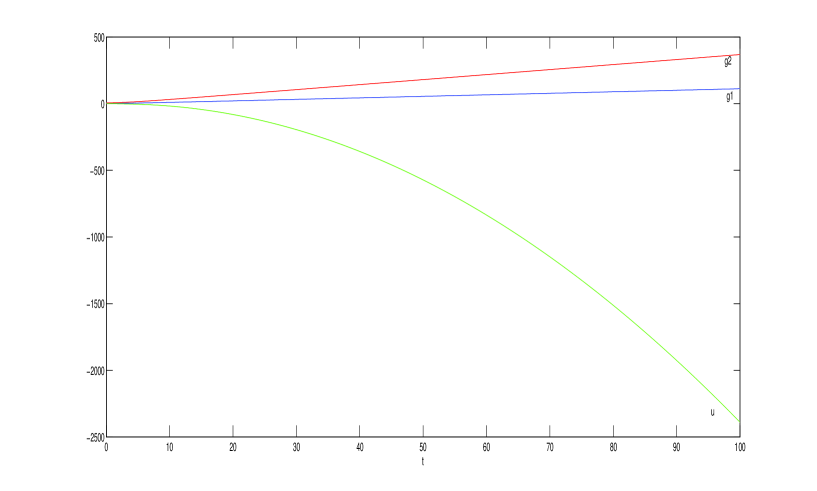
Figure 1. $m=1$ case

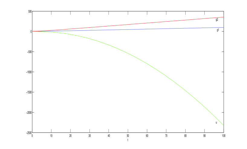
Figure 2. $m=2$ case

We have also plotted the quantities ${\tilde{X}}_{i}=\frac{X_{i}}{\sqrt{d_{i}}}$ and ${\tilde{Y}}_{i}=\frac{Y_{i}}{\sqrt{d_{1}}}$ against $t$ in Figures 3 and 4 for the $m=1$ and $m=2$ cases respectively. They all converge quickly to $0$.

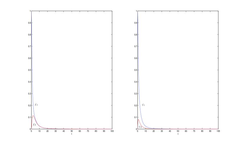
Figure 3. $m=1$ case

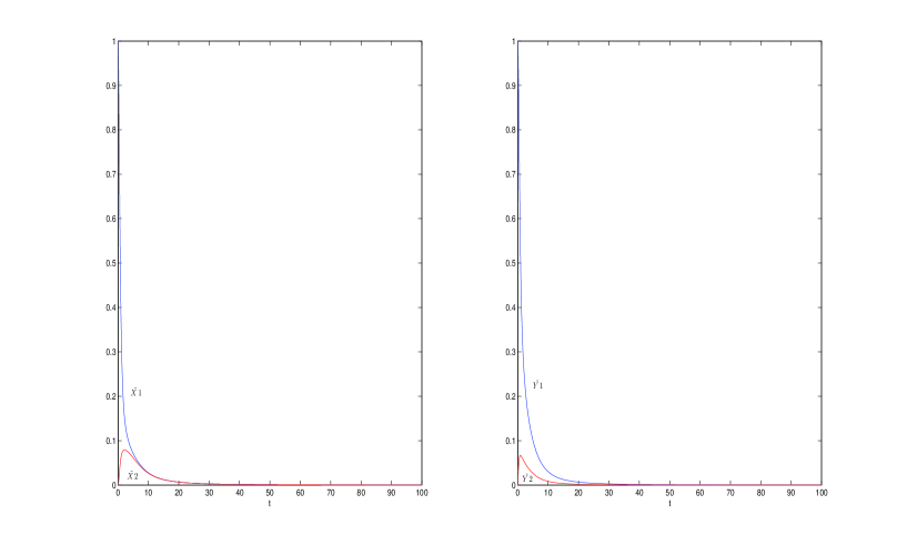
Figure 4. $m=2$ case

In Figure 5 we plot the ratios ${\tilde{X}}_{1}/{\tilde{X}}_{2}$ and ${\tilde{Y}}_{1}/{\tilde{Y}_{2}}$. Note that the second ratio is $\frac{g_{2}}{g_{1}}$, which tends to a positive constant. The first ratio is the ratio of the principal curvatures $\frac{\dot{g}_{2}}{g_{2}}/\frac{\dot{g}_{1}}{g_{1}}$ and we see that it quickly approaches $1$.

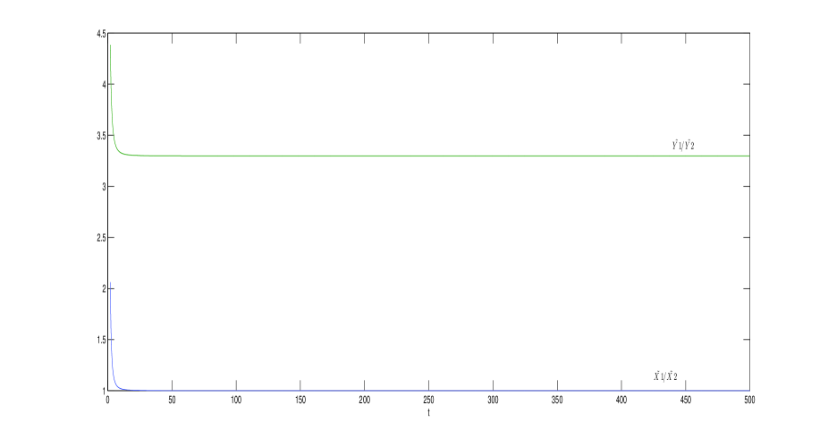
Figure 5.

Similar numerical results hold for larger values of $m$.

Example 2.   We next set $G={\rm Sp}(m+1)\times{\rm Sp}(1),H={\rm Sp}(m)\times{\rm Sp}(1)\times{\rm Sp}(1),$ and $K={\rm Sp}(m)\times\Delta{\rm Sp}(1)$. The principal orbit $G/K$ is diffeomorphic to $S^{4m+3}$ and the singular orbit $G/H$ is again $\mbox{${\mathbb{H}}$}{\mbox{${\mathbb{P}}$}}^{m}$. So $d_{1}=3,d_{2}=4m$, and $A_{2}=4m(m+2),A_{3}=\frac{3m}{4}$ (where $\mathsf{b}$ is given by $-2{\rm tr}(XY)$ on both of the simple factors). The initial values of $(z_{1},\ldots,z_{6})$ are given by $(0,1,\bar{h},0,\bar{u},0)$ where $\bar{h}>0$ and $\bar{u}<0$.

For this case we obtain graphs very similar to those in Example 1.

Based on the last two examples, we would conjecture that on the vector bundles $G\times_{H}\mbox{${\mathbb{R}}$}^{d_{1}+1},$ where $(G,H,K)$ are as above, there is a $2$-parameter family of non-homothetic complete expanding gradient Ricci solitons.

References

- [BB] L. Bérard Bergery, Sur des nouvelles variétés Riemanniennes d’Einstein, Publications de l’Institut Elie Cartan, Nancy, (1982).
- [Bo] C. Böhm, Non-compact cohomogeneity one Einstein manifolds, Bull. Soc. Math. France, 122, (1999), 135-177.
- [BGK1] C. Boyer, K. Galicki and J. Kollár, Einstein metrics on spheres, Ann. Math., 162, (2005), 557-580.
- [BGK2] C. Boyer, K. Galicki and J. Kollár, Einstein metrics on exotic spheres in dimension and , Experiment. Math., 14, (2005), 59-64.
- [Bry] R. Bryant, unpublished work.
- [Buz] M. Buzano, Initial value problem for cohomogeneity one gradient Ricci solitons, J. Geom. Phys, 61, (2011), 1033-44.
- [BDGW] M. Buzano, A. Dancer, M. Gallaugher and M. Wang, A family of steady Ricci solitons and Ricci-flat metrics, arXiv:math.DG//1309.6140.
- [Cao] H. D. Cao, Existence of gradient Ricci solitons, Elliptic and Parabolic Methods in Geometry, A. K. Peters, (1996), 1-16.
- [CaNi] J. A. Carrillo and L. Ni, Sharp logarithmic Sobolev inequalities on gradient solitons and applications, Comm. Anal. Geom., 17, (2009), 721-753.
- [Chb] B. L. Chen, Strong uniqueness of the Ricci flow, J. Diff. Geom., 82 , (2009),363-382.
- [Chc] Chih-Wei Chen, On the asymptotic behavior of expanding gradient Ricci solitons,, Ann. Glob. Anal. Geom., 42, (2012), 267-277.
- [Cho] O. Chodosh, Expanding Ricci solitons asymptotic to cones, arxiv:math.DG//1303.2983.
- [DHW] A. Dancer, S. Hall and M. Wang, Cohomogeneity one shrinking Ricci solitons: an analytic and numerical study, Asian J. Math., 17, (2013), no. 1, 33-61.
- [DW1] A. Dancer and M. Wang, On Ricci solitons of cohomogeneity one, Ann. Glob. Anal. Geom., 39, (2011) 259-292.
- [DW2] A. Dancer and M. Wang, Some new examples of non-Kähler Ricci solitons, Math. Res. Lett. 16, (2009) 349-363.
- [DW3] A. Dancer and M. Wang, Non-Kähler expanding Ricci solitons, IMRN, (2009), 1107-33.
- [DW4] A. Dancer and M. Wang, The cohomogeneity one Einstein equations from the Hamiltonian viewpoint, J. reine angew. Math., 524, (2000), 97-128.
- [FR] M. Fernández-López and E. García-Río, Maximum principles and gradient Ricci solitons, J. Diff. Equations, 251, (2011), 73-81.
- [Gaf] M. P. Gaffney, A special Stoke’s theorem for complete Riemannian manifolds, Ann. Math., 60, (1954), 140-145.
- [GK] A. Gastel and M. Kronz, A family of expanding Ricci solitons, Variational Problems in Riemannian Geometry, Prog. Nonlinear Differential Equations Appl. 59, Birkhäuser, Basel (2004), 81–93.
- [GHMS] M. Gutperle, M. Headrick, S. Minwalla and V. Schomerus, Space-time energy decreases under world-sheet RG flow, JHEP, 1 (2003).
- [Iv] T. Ivey, New examples of complete Ricci solitons, Proc. AMS, 122, (1994), 241-245.
- [Ja] M. Jablonski, Homogeneous Ricci solitons, arXiv:math.DG//1109.6556.
- [Ka] K. Kawakubo, Smooth structures on , Osaka J. Math., 6, (1969), 165-196.
- [KwS] S. Kwasik and R. Schultz, Multiplication stablization and transformation groups, in Current Trends in Transformation Groups, K-Monogr. Math., Kluwer, (2002), 147-165.
- [La1] J. Lauret, Ricci soliton homogeneous nilmanifolds, Math. Ann., 319 (2001), 715-733.
- [La2] J. Lauret, Einstein solvmanifolds and nilsolitons, Contemporary Mathematics, 491, (2009), 1-35.
- [La3] J. Lauret, Ricci soliton solvmanifolds, J. reine angew. Math., 650, (2011), 1-21.
- [MS] O. Munteanu and N. Sesum, On gradient Ricci solitons, J. Geom. Anal. 23, (2013), no. 2, 539-561.
- [PW] P. Petersen and W. Wylie, Rigidity of gradient Ricci solitons, Pacific J. Math., 241, (2009), 329-345.
- [PrW] M. Protter and H. Weinberger, Maximum principles in differential equations, Springer-Verlag, (1984).
- [PRS] S. Pigola, M. Rimoldi and A. Setti, Remarks on non-compact gradient Ricci solitons, Math. Z., 268, (2011), 777-790.
- [Sc] R. Schultz, Smooth structures on , Ann. Math., 90, (1969), 187-198.
- [SS] F. Schulze and M. Simon, Expanding solitons with non-negative curvature operator coming out of cones, Math. Z., 275, (2013), no. 1-2, 625-639.
- [Y] S. T. Yau, Some function-theoretic properties of complete Riemannian manifold and their applications to geometry, Indiana U. Math. J., 25, (1976), 659-670.
- [Zh] Z.-H. Zhang, On the completeness of gradient Ricci solitons, Proc. A. M. S., 137, (2009), 2755-2759.