Testing metallicity indicators at $z\sim 1.4$ with the gravitationally lensed galaxy CASSOWARY 20

Abstract

We present X-shooter observations of CASSOWARY 20 (CSWA 20), a star-forming (SFR $\sim 6$ M_⊙ yr^-1) galaxy at $z=1.433$, magnified by a factor of 11.5 by the gravitational lensing produced by a massive foreground galaxy at $z=0.741$. We analysed the integrated physical properties of the H ii regions of CSWA 20 using temperature- and density-sensitive emission lines. We find the abundance of oxygen to be $\sim 1/7$ of solar, while carbon is $\sim 50$ times less abundant than in the Sun. The unusually low C/O ratio may be an indication of a particularly rapid timescale of chemical enrichment. The wide wavelength coverage of X-shooter gives us access to five different methods for determining the metallicity of CSWA 20, three based on emission lines from H ii regions and two on absorption features formed in the atmospheres of massive stars. All five estimates are in agreement, within the factor of $\sim 2$ uncertainty of each method. The interstellar medium of CSWA 20 only partially covers the star-forming region as viewed from our direction; in particular, absorption lines from neutrals and first ions are exceptionally weak. We find evidence for large-scale outflows of the interstellar medium (ISM) with speeds of up 750 km s^-1, similar to the values measured in other high-$z$ galaxies sustaining much higher rates of star formation.

1 Introduction

Constraining the degree of metal enrichment in the Universe is of paramount importance for our understanding of galaxy formation and evolution. The metallicity of a galaxy reflects its evolutionary state, and the most abundant chemical elements regulate many of the astrophysical processes that drive star formation and galaxy evolution: cooling, formation of dust and molecules, the opacity and energy transport within stellar atmospheres and the synthesis of new nuclei within stars.

In galaxies that are actively forming stars, element abundances have mostly been determined by modelling the relative strengths of emission lines from H ii regions, including weak, temperature-sensitive transitions such as [O iii] $\lambda$4363.44 and [N ii] $\lambda$5756.24 (vacuum wavelengths). This is often referred to as the ‘direct’, or ‘$T_{\rm e}$’, method. Unfortunately, these auroral lines become increasingly difficult to detect in distant, faint galaxies due to the limited sensitivity of current instrumentation compounded with the strong sky background at near-infrared wavelengths, where the lines fall at redshifts $z\gtrsim 1.2$. Furthermore, most galaxies at $z>1$ with measurements of rest-frame optical emission lines are fairly luminous, and, accordingly, not extremely metal poor. Since temperature-sensitive auroral features decline in strength strongly with increasing metallicity, these features are intrinsically weak in the majority of high-redshift galaxies studied to date.

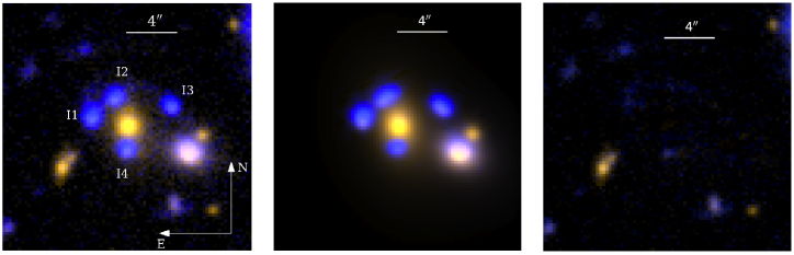
Figure 1: Left: Colour composite of $g$ and $i$ images of the CSWA 20 lens system. The images were obtained with the Auxiliary Port camera of the William Herschel Telescope (WHT) on La Palma; the exposure times were 300 s in each band and the seeing was $\sim 0.8$ arcsec FWHM. Superposed on the image is an outline of the entrance slit of X-shooter, at the two orientations used (Table LABEL:tab:obs).  Centre: Image-plane reconstruction of CSWA 20 with the lensing model described in Section 2.3. Photometry of the system is collected in Table 1. Right: Residuals from subtracting the model (centre) from the data (left).

In such cases, we are forced to rely on metallicity ‘indicators’ which involve the ratios of strong emission lines. The most widely used of these ‘strong-line’, or ‘empirical’, methods is the $R_{23}$ index which relates the abundance of oxygen to the ratio of ([O iii] $\lambda\lambda 5008.24,4960.30$ + [O ii] $\lambda\lambda 3727.09,3729.88$) to H$\beta$$\lambda 4862.69$ (Pagel et al. 1979). Other combinations of emission lines have been proposed and extensively used at high redshifts (e.g. Maiolino et al. 2008); among these, the $N2$ index ([N ii]$\lambda 6585.23$/H$\alpha\lambda 6564.61$) of Pettini & Pagel (2004) has turned out to be particularly useful for obtaining a rough measure of a galaxy’s metallicity at redshifts $z\sim 2.3$, where observations from the ground can capture all the main nebular emission lines in the near-infrared atmospheric transmission windows. This coincidence is especially convenient given that $z\sim 2.3$ corresponds to the epoch when the Universal star-formation rate was at its peak (Madau & Dickinson 2014).

While these and other strong-line indices have been calibrated with reference to abundances measured by the ‘direct’ method, it is a matter of concern that different calibrations are not always in agreement and can yield widely different values of the oxygen abundance (Kewley & Ellison 2008). To make matters worse, it is now clear that the physical conditions of the most actively star-forming galaxies at $z\gtrsim 2$ are significantly more extreme (higher densities of matter and photons, and harder radiation fields) than found locally (Hainline et al. 2009; Steidel et al. in preparation). It is therefore questionable to what extent the local empirical metallicity indicators can be reliably applied to high-$z$ galaxies.

In order to make progress on some of these issues, it would be highly desirable to compare, for the same galaxy, element abundances derived with different methods. At high redshift, there have so far been only a handful of cases where the ‘direct’ and ‘empirical’ methods for measuring the oxygen abundance could be compared (Villar-Martín et al. 2004; Yuan & Kewley 2009; Erb et al. 2010; Christensen et al. 2012). Generally, the two sets of values of O/H have been found to agree within the errors, although in one case (Yuan & Kewley 2009) the detection of [O iii] $\lambda 4364.44$ in a gravitationally lensed galaxy at $z=1.705$ led to a downward revision by a factor of about four in the oxygen abundance compared to the value estimated from the $R_{23}$ index.

Table 1: $g$ and $i$ magnitudes of CSWA 20.^a

Image	$g^{\rm b}$	$i^{\rm c}$
I1	21.91	21.87
I2	22.25	22.32
I3	22.49	22.49
I4	22.47	22.42
Total	20.75	20.74

^a Measured from the WHT images and lensing model shown in Figure 1.
^b Systematic error on the zero-point of the photometry is $\pm 0.1$ mag.
^c Systematic error on the zero-point of the photometry is $\pm 0.17$ mag.

The limitations in the use of nebular abundance diagnostics at high redshifts have motivated the exploration of alternative metallicity measures based on spectral features in the rest-frame ultraviolet (UV) range, including interstellar absorption lines (Pettini et al. 2002), P-Cygni emission-absorption features arising from the winds of the most luminous early-type stars (Leitherer et al. 2010, and references therein), and photospheric absorption lines from OB stars [Rix et al. (2004) and references therein; see also Maraston et al. (2009)]. A comparison of these different methods in the very few cases where it was possible can be found in Pettini (2006); see also Halliday et al. (2008) and Sommariva et al. (2012). These UV-based methods are still in the development stage and are currently less accurate than the emission line diagnostics. Some of the difficulties in their use are: (i) the fact that some of the photospheric features are blends of lines from different ions, (ii) the dependence of the stellar wind lines on the age of the starburst and on the initial mass function (IMF), and (iii) complications in separating stellar and interstellar contributions (Crowther et al. 2006). However, they do offer the hope of determining metal abundances of galaxies out to $z\sim 7$, where the emission lines from H ii  regions are redshifted beyond the reach of ground-based telescopes (although the UV diagnostics require detecting the stellar continuum, which is beyond current capabilities for galaxies at $z\gtrsim 5$).

The ability to detect weak emission lines and, more generally, to compare different metallicity indicators, can be greatly facilitated by gravitational lensing which makes it possible to record the spectra of high-$z$ galaxies at higher signal-to-noise ratio (S/N) and resolution than would otherwise be the case. For this reason, most of the examples cited above refer to gravitationally lensed galaxies.

While such cases are still relatively rare, their numbers have increased substantially in recent years through dedicated searches in large sky surveys, such as the Sloan Digital Sky Survey (SDSS) — eg. Kubo et al. (2009, and references therein); see also Richard et al. (2011) and Stark et al. (2013) for other recent examples. The CAmbridge Sloan Survey Of Wide ARcs in the skY (CASSOWARY) targets multiple, blue companions around massive ellipticals in the SDSS photometric catalogue as likely candidates for wide separation gravitational lens systems (Belokurov et al. 2009). The twentieth source in the CASSOWARY catalogue, CSWA 20, was confirmed by Pettini et al. (2010) to be four images of the same $z_{\rm em}=1.433$ star-forming galaxy separated by $\sim 3$–5″  by the gravitational potential of a foreground $z_{\rm abs}=0.741$ massive red galaxy (see Figure 1).

Following these initial observations, we targeted CSWA 20 in a dedicated programme using the X-shooter spectrograph on the Very Large Telescope (VLT) of the European Southern Observatory (ESO), with the aim of recording the galaxy spectrum at sufficient resolution and S/N for a detailed study of its physical properties and, in particular, testing the consistency of different metallicity measures. The results of this work are presented here.

The organisation of the paper is as follows. In Section 2 we describe the X-shooter observations and data reduction; we also give a brief description of the lensing model. The full CSWA 20 X-Shooter spectrum is presented in Section 3, along with our analysis of its emission and absorption lines. Sections 4 and 5 deal with the measurements of element abundances by different methods; the results are compared in Section 6. The main conclusions of this work are summarised in Section 7.

2 Observations and Data Reduction

2.1 Observations

The X-shooter spectrograph (Vernet et al. 2011) delivers medium resolution spectra obtained simultaneously from three separate arms: UVB (300–550 nm), VIS (550–1015 nm) and NIR (1025–2400 nm). Our observations of CSWA 20 used entrance slits of 1.0 arcsec (UVB), 0.9 arcsec (VIS) and 0.9 arcsec (NIR), with corresponding resolving powers of $R=\lambda/\Delta\lambda\sim 4400$, 7500 and 5300, sampled with $\sim 5.5$, 7.1 and 4.2 pixels respectively (after on-chip binning by a factor of two on the UVB and VIS detectors).

Two orientations of the spectrograph slits on the sky were used, the first at position angle PA $=-53^{\circ}$ to record simultaneously the spectrum of images I1 and I2 (see Figure 1), and the second at PA $=-46^{\circ}$ covering I3 and I4. The observations used a nodding along the slit approach, with an offset of 4 arcsec between individual exposures; typically each observation consisted of four 900 s exposures in a ABBA pattern. A journal of observations is given in Table LABEL:tab:obs. Although our plan was to divide the allocated exposure time equally between the two slit settings, this service programme was terminated by ESO before it had been completed. Consequently, the spectra secured are mostly those of images I1 and I2 (see Table LABEL:tab:obs).

Table 2: Journal of observations.

Date (UT)	Exposure time (s)	Slit PA($\deg$)	Target
2011 May 07	4 $\times$ 900	53	I1 & I2
2011 July 29	4 $\times$ 900	53	I1 & I2
2011 June 27	4 $\times$ 900	53	I1 & I2
2011 May 29	4 $\times$ 900	53	I1 & I2
2011 May 23	4 $\times$ 900	53	I1 & I2
2011 May 10	4 $\times$ 900	53	I1 & I2
2011 April 29	4 $\times$ 900	53	i1 & i2
2011 April 09	8 $\times$ 900	53	I1 & I2
2011 May 07	2 $\times$ 600	46	I3 & I4
2011 August 03	4 $\times$ 900	46	I3 & I4

2.2 Data Reduction

The X-shooter spectra were reduced with a suite of customised routines designed to optimally subtract the sky background and extract one-dimensional spectra while minimising the noise (Kelson 2003; Becker et al. 2009). For each observation listed in Table LABEL:tab:obs, we extracted separately the spectrum of each image on the slit; this resulted in 84 individual 1-D spectra for each of the three arms of X-shooter. Of these, $\sim 80$ were usable (in four cases one of the images fell too close to the slit edge to allow accurate sky subtraction).

Wavelength calibration used reference spectra of a Th-Ar hollow-cathode lamp, with small adjustments to the wavelength solution, when required, to match the wavelengths of emission lines from the night sky. At the S/N ratio of our data, no significant differences were found between the spectra of the different images, and indeed none are expected from the reconstruction of the source (see Section 2.3). Therefore we combined all 80 spectra with S/N weighting to produce a total spectrum in each arm. From the rms deviations of the data in regions free of obvious spectral features we measure S/N $\simeq 8$, 15 and 5 for the final spectrum in the UVB, VIS and NIR arms respectively.

The spectra were not corrected for telluric absorption because no emission or absorption lines of interest were affected. For flux calibration, we scaled the X-shooter final VIS arm spectrum to match the $i$-band magnitude measured from the WHT images (Figure 1 and Table 1) and the $r$-band magnitude measured from the X-shooter acquisition images. Using spectral overlap regions, the UVB and NIR spectra were then scaled accordingly to the flux-calibrated VIS spectrum. Uncertainties resulting from flux calibration were estimated to be $\sim 10$%.

2.3 Lensing Model

The gravitational lens model was determined by fitting a singular isothermal ellipsoid (SIE) mass model with external shear to the WHT $g$ and $i$ imaging data shown in Figure 1, following the procedure outlined in Stark et al. (2013) and Auger et al. (2013). The source was modelled as a single Sersic component; the right panel in Figure 1 shows the reconstructed image of the system. We find that our model agrees well with the model from Pettini et al. (2010), and in particular we note that our derived SIE velocity dispersion of 496 km s^-1 is in excellent agreement with the spectroscopic velocity dispersion of the lensing galaxy. The mass distribution traces the light well, as each has a flattening of $\sim 0.7$, and we find a significant external shear of $0.18$ oriented at a position angle of 18 degrees.

We find the total lensing magnification to be $f=11.5$, $\approx 2-4$ times higher than the initial approximate estimate given by Pettini et al. (2010). This value of $f$ is very precisely determined within the context of our model (the statistical uncertainty from our modelling is less than 1%). However, although our lensing model reproduces the CSWA 20 configuration very well (see Figure 1), it is not unique. Furthermore, as is the case with most lensing models, there may be significant systematic uncertainties due to differential magnification of structure within the source. Indeed, the magnifications inferred from the $g$ and $i$ bands differ by $10\%$, possibly signalling differential magnification, and we therefore impose a systematic uncertainty of $\pm 10\%$ on the fluxes used throughout our analysis.

Table 3: Emission line fit parameters.

Parameter	Narrow	Broad
High S/N lines:
$z$	$1.433485$	$1.433074$
	$\pm 0.000004$	$\pm 0.000023$
Velocity offseta (km s-1)	0.0	$-51\pm 3$
$\sigma$(km s -1)	$34.9\pm 0.7$	$109\pm 3$
Mg ii $\lambda\lambda$2796,2803:
$z$	1.43377	1.43335
	$\pm 0.00002$	$\pm 0.00005$
Velocity offseta (km s-1)	$+35\pm 3$	$-17\pm 6$
$\sigma$(km s -1)	$40\pm 2$	$108\pm 5$

^a Relative to $z=1.433485$, taken to be the systemic redshift.

3 The Spectrum

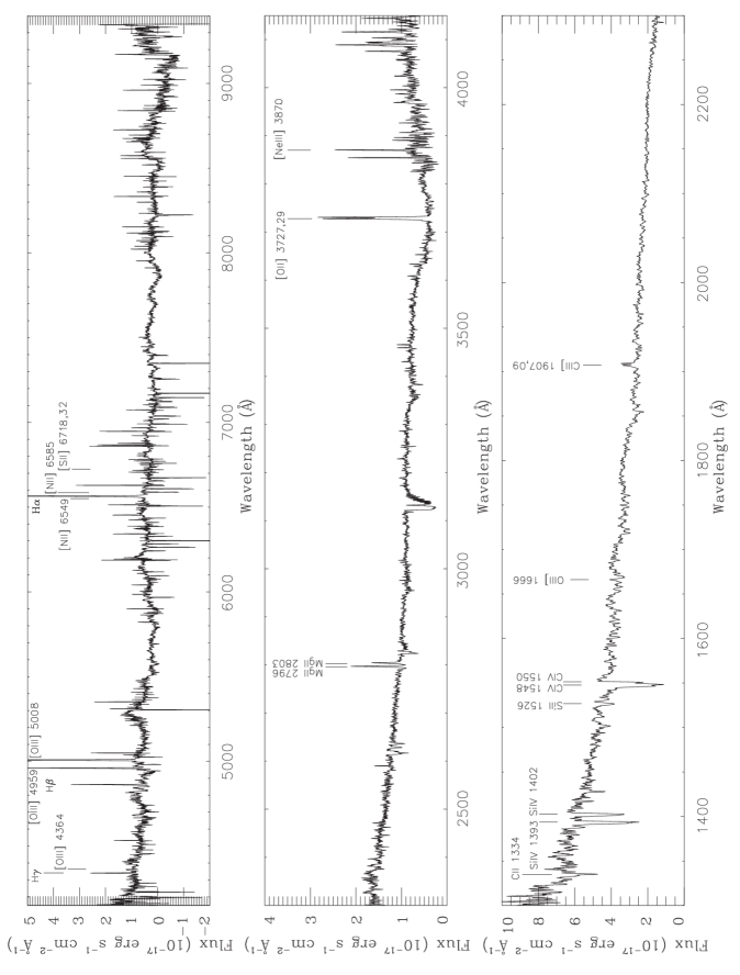
Figure 2: X-Shooter spectrum of CSWA 20 with the most important emission and absorption lines labelled; top panel: NIR arm, middle panel: VIS arm, and bottom panel: UVB arm. Wavelengths are given in the rest frame of the gravitationally lensed galaxy at $z_{\rm em}=1.4335$. Each spectrum has been smoothed with a 5-pixel boxcar for presentation purposes.

Figure 2 shows the complete, flux-calibrated X-Shooter spectrum of CSWA 20. The spectrum exhibits all the strong emission lines typical of star-forming galaxies, superimposed on a blue continuum. On the other hand, the UV absorption spectrum is unusual, in that most interstellar lines are much weaker than is normally the case in star-forming galaxies at these redshifts (e.g. Steidel et al. 2004; Erb et al. 2010; Martin et al. 2012; Kornei et al. 2013). In this Section, we describe the main characteristics of the spectrum of CSWA 20, focussing on the emission lines in Section 3.1, and on the absorption lines in Section 3.2.

Table 4: Observed and de-reddenened line fluxes relative to H$\beta$.^a

	$F_{\lambda}$	$I_{\lambda}$
O iii] $\lambda 1660.81$	0.04 $\pm$ 0.04	0.11 $\pm$ 0.11
O iii] $\lambda 1666.15$	0.10 $\pm$ 0.04	0.26 $\pm$ 0.13
[C iii] $\lambda 1906.68$	0.12 $\pm$ 0.01	0.28 $\pm$ 0.08
C iii] $\lambda 1908.73$	0.11 $\pm$ 0.01	0.25 $\pm$ 0.07
Mg ii $\lambda 2796.36$	0.22 $\pm$ 0.01	0.33 $\pm$ 0.05
Mg ii $\lambda 2803.53$	0.15 $\pm$ 0.01	0.22 $\pm$ 0.03
[O ii] $\lambda 3727.10$	0.47 $\pm$ 0.02	0.55 $\pm$ 0.04
[O ii] $\lambda 3729.86$	0.52 $\pm$ 0.03	0.62 $\pm$ 0.05
[Ne iii] $\lambda 3870.16$	0.37 $\pm$ 0.02	0.43 $\pm$ 0.03
H$\gamma$ $\lambda 4341.69$	0.57 $\pm$ 0.05	0.61 $\pm$ 0.06
[O iii] $\lambda 4364.44$	0.05 $\pm$ 0.03	0.05 $\pm$ 0.03
H$\beta$ $\lambda 4862.69$	1.00 $\pm$ 0.07	1.00 $\pm$ 0.07
[O iii] $\lambda 4960.30$	1.67 $\pm$ 0.10	1.65 $\pm$ 0.10
[O iii] $\lambda 5008.24$	4.97 $\pm$ 0.29	4.88 $\pm$ 0.28
[N ii] $\lambda 6549.85$	0.02 $\pm$ 0.04	0.02 $\pm$ 0.03
H$\alpha$ $\lambda 6564.61$	3.32 $\pm$ 0.20	2.78 $\pm$ 0.24
[N ii] $\lambda 6585.27$	0.06 $\pm$ 0.02	0.05 $\pm$ 0.02
[S ii] $\lambda 6718.29$	0.06 $\pm$ 0.03	0.05 $\pm$ 0.03
[S ii] $\lambda 6732.67$	0.12 $\pm$ 0.02	0.10 $\pm$ 0.02
$F$(H$\beta$)	$(2.38\pm 0.12)\times 10^{-16}$ erg s-1 cm-2
$I$(H$\beta$)	$(4.21\pm 0.34)\times 10^{-16}$ erg s-1 cm-2
$E(B-V)$	$0.17\pm 0.06$ mag

^a Vacuum wavelengths.

3.1 Emission lines

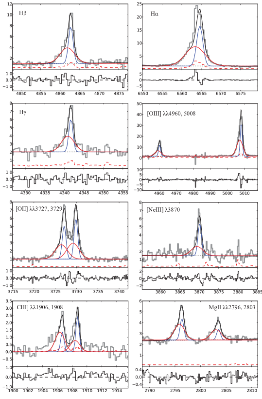
Figure 3: High S/N emission lines observed within the X-shooter wavelength range. In each panel, the $x$-axis is the rest-frame wavelength in Å, and the $y$-axis is the observed flux in units of $10^{-17}$ erg s^-1 cm^-2 Å^-1. In each plot, the grey histogram is the observed spectrum, and the red dashed line is the $1\sigma$ error spectrum. Overplotted on the data we show separately the best-fit profiles for the narrow (blue solid line), and broad (red solid line) emission components; their sum is shown with the black solid line. Relevant parameters of the model fit are given in Table LABEL:tab:params, and the total line fluxes are listed in Table 4. Underneath each emission line we show the difference between the data and the best-fit model.

In Figure 3 we have collected the strongest emission lines observed in our spectrum. All of them exhibit asymmetric profiles, with an extended blue wing. We have modelled these lines with two separate Gaussian components (the minimum required for a satisfactory fit), to deduce their redshifts and velocity dispersions, as well as the total integrated line flux of each emission line. Results of the model fits are collected in Tables LABEL:tab:params and 4.

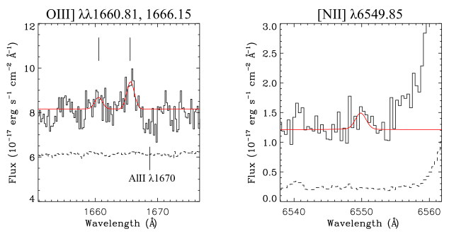
Figure 4: Example of weak emission lines near, or below, the detection limit of the X-shooter spectrum of CSWA 20. O iii] $\lambda 1666.15$ is detected at the $\sim 3\sigma$ level, while O iii] $\lambda 1660.81$ and [N ii] $\lambda 6549.85$ are comparable to the noise (see Table 4). The data are the black histogram and the model fit is shown by the red continuous line. The dashed line is the error spectrum; in the case of the O iii] doublet (left panel), we have added a constant factor of $5\times 10^{-17}$ erg s^-1 cm^-2 Å^-1 to the noise spectrum in order to bring it within the range of the plot. Also marked on this plot is the interstellar Al ii absorption line.

All of the emission lines shown in Figure 3 were fitted simultaneously (with the exception of the Mg ii doublet for the reasons given below), to ensure consistent kinematic measurements, (i.e., we required the redshifts and line widths of each emission component to be the same for all the lines fitted). The model included four non-linear parameters (the redshifts $z$ and velocity dispersions $\sigma$ of each velocity component) that were determined by a Markov chain Monte Carlo (MCMC) method, while the fluxes in each emission component were treated as linear parameters. For each MCMC step we solved the bounded linear problem that determines the (non-zero) amplitude of each line given the current values for the non-linear parameters; we explicitly accounted for the uncertainties from the linear inversion by attaching samples for the inference of the line amplitudes to the MCMC chain.

The Mg ii $\lambda\lambda 2796,2803$ doublet lines were fitted separately from the other strong emission lines because, being resonance lines, they are potentially a mix of absorption and emission. Indeed, in galaxies hosting large-scale outflows of the interstellar medium (ISM), these lines can exhibit P-Cygni profiles, akin to those more commonly seen in Ly$\alpha$ (Rubin et al. 2010; Kornei et al. 2013). The finding that in CSWA 20 the Mg ii doublet is mostly in emission (see bottom right panel of Figure 3) is likely to be a consequence of the unusually low optical depth in this galaxy of interstellar absorption lines from neutral, or mildly ionised, gas, as discussed below (Section 3.2). As can be seen from Table LABEL:tab:params and Figure 3, the Mg ii lines also consist of two components, with velocity dispersions which are broadly consistent with those determined for the nebular lines within the errors. On the other hand, the velocities of the two components are higher than those of the nebular lines by $\sim 35$ km s^-1, probably as a result of resonant scattering.

In addition to the emission lines collected in Figure 3, the X-shooter spectrum covers a number of other weak emission lines which are near, or below, the detection limit. Three examples are reproduced in Figure 4. The fluxes of these weak features are included in Table 4; they were measured by fitting to the data theoretical profiles with the model parameters determined for the high S/N emission lines, as listed in Table LABEL:tab:params.

3.1.1 Reddening and star-formation rate

From Table 4 it can be seen that we measure $F$(H$\alpha$)/$F$(H$\beta$)$=3.32\pm 0.20$. Adopting the case B recombination ratio $F$(H$\alpha$)/$F$(H$\beta$)$=2.78$ from Brocklehurst (1971), appropriate to gas with $T=17\,000$ K and $n{\rm(e)}=300$ cm^-3 as derived below for CSWA 20 (see Section 4.1), and the LMC extinction curve (Fitzpatrick 1999), we find that the Balmer decrement implies a reddening $E(B-V)=0.17\pm 0.06$ mag.

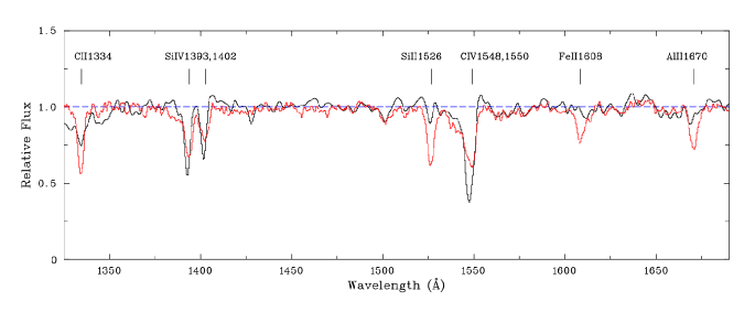
Figure 5: Comparison of portion of the normalised spectrum of CSWA 20 (black histogram) with the median spectrum of $\sim 380$ ‘BM’ star-forming galaxies at $z\simeq 1.4$–2.0 from the surveys by Steidel et al. (2004), shown in red. Interstellar lines of interest are indicated. The X-shooter spectrum of CSWA 20 has been smoothed and rebinned to match the $\sim 2.5$ Å resolution of the BM composite.

Table 5: Interstellar Absorption Lines.

Line ID	$\lambda_{\rm lab}^{\rm a}$ (Å)	$f$-valuea	$\lambda_{\rm c}^{\rm b}$ (Å)	$v^{\rm c}$ (km s-1)	$\Delta v^{\rm d}$	$W_{0}^{\rm e}$ (Å)
C ii $\lambda 1334$	1334.5323	0.1278	1334.17	$-81$	$-540$ to $+270$	$0.63\pm 0.07$
C iv $\lambda 1548$	1548.2041	0.1899	…	…	$-740$ to $+190$	$3.44\pm 0.07^{\rm f}$
C iv $\lambda 1550$	1550.7812	0.09475	…	…	$-740$ to $+190$	$3.44\pm 0.07^{\rm f}$
Si ii $\lambda 1526$	1526.7070	0.133	1526.04	$-131$	$-540$ to $+270$	$0.52\pm 0.07$
Si iv $\lambda 1393$	1393.7602	0.513	1392.61	$-248$	$-740$ to $+190$	$1.78\pm 0.06$
Si iv $\lambda 1402$	1402.7729	0.254	1401.57	$-257$	$-740$ to $+190$	$1.48\pm 0.06$
Al ii $\lambda 1670$	1670.7886	1.74	1669.54	$-224$	$-540$ to $+270$	$0.36\pm 0.07$
Al iii $\lambda 1854$	1854.7184	0.559	1853.30	$-229$	$-740$ to $+190$	$0.65\pm 0.08$
Al iii $\lambda 1862$	1862.7910	0.278	1860.75	$-329$	$-740$ to $+190$	$0.42\pm 0.08$

Notes:

^a Rest vacuum wavelengths and $f$-values from Morton (2003).

^b Centroid rest-frame wavelength.

^c Velocity relative to systemic, at $z_{\rm em}$=1.433485.

^d Velocity range for equivalent width measurements relative to $z_{\rm em}$=1.433485.

^e Rest-frame equivalent width and $1\sigma$ error.

^f Refers to C iv $\lambda$1549 doublet.

With the adoption of the conventional $\Omega_{\rm M}=0.3$, $\Omega_{\Lambda}=0.7$, $h=0.7$ cosmological parameters, the reddening-corrected H$\alpha$ flux we measure in CSWA 20 (Table 4), corresponds to a luminosity $L{\rm(H}\alpha)=(1.49\pm 0.13)\times 10^{43}$ erg s^-1. This value can be converted into a star formation rate:

$${\rm SFR(H\alpha)}=7.9\times 10^{-42}L({\rm H}\alpha)\times\frac{1}{1.8}\times\frac{1}{11.5}=(5.7\pm 0.5)\,{\rm M}_{\odot}~{}{\rm yr}^{-1}$$ (1)

where the first factor on the right-hand side of the equation is Kennicutt’s (1998) calibration appropriate to a Salpeter initial mass function, corrected for the more realistic turn-over at low masses proposed by Chabrier (2003) (amounting to a factor of 1.8), and for the 11.5 magnification factor returned by our lensing model. (Note that an additional systematic error of 10% applies to all our estimates of line luminosity and SFR from the 10% uncertainty in the magnification factor – see Section 2.3). The value of SFR in equation (1) is $\sim 3.7$ times smaller than that deduced by Pettini et al. (2010), mainly as a result of the better modelling of the lens system performed here.

The star formation rate can also be deduced from the luminosity of the UV continuum produced by OB stars. From the spectrum in Figure 2, we measure $F_{\lambda}(1500)=(4.7\pm 0.5)\times 10^{-17}$ erg s^-1 cm^-2 Å^-1 by averaging over a 40 Å window centred at 1500 Å away from obvious emission and absorption lines. (The error quoted is from the $\sim 10$% uncertainty in our flux calibration—see Section 2.2). In our cosmology, this corresponds to a continuum luminosity density at 1500 Å: $L_{\nu}=(9.2\pm 4.4)\times 10^{29}$ erg s^-1 Hz^-1, after correcting for the attenuation at 1500 Å according to Calzetti et al. (2000). (The error now includes the uncertainty in $E(B-V)$, added in quadrature). In turn, this leads to:

$${\rm SFR(UV)}=1.4\times 10^{-28}L_{\nu}{\rm(UV)}\times\frac{1}{1.8}\times\frac{1}{11.5}=(6\pm 3)\,{\rm M}_{\odot}~{}{\rm yr}^{-1}$$ (2)

following the same reasoning as in equation (1).

The larger error in SFR(UV) compared to SFR(H$\alpha$) arises from the larger uncertainty in the attenuation at 1500 Å compared to the attenuation at H$\alpha$. The two estimates of the SFR are in good agreement. It is not unexpected, however, for the two estimates to differ by a factor of $\sim 2$, given the many assumptions involved (including that the UV and H$\alpha$ luminosities track each other, which is only the case in the ideal scenario of continuous star formation at a constant rate). Differences by factors of $\sim 2$ between SFR(H$\alpha$) and SFR(UV) are commonly found in such estimates at high $z$ (e.g. Erb et al. 2006b).

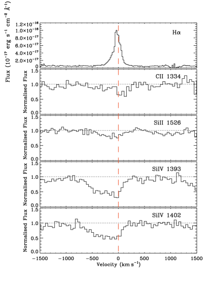
Figure 6: Normalised profiles of selected interstellar absorption lines in CSWA 20, compared to the H$\alpha$  emission line (top panel). The $x$-axis gives velocity relative to $z_{\rm sys}=1.433485$, as derived from the nebular emission lines (Section 3.1).

3.2 Absorption lines

It may be appreciated from inspection of Figure 2 that very few interstellar absorption lines seem to be present in the UV spectrum of CSWA 20. The main reason is the unusual weakness of absorption lines from neutrals and the first ions that are the main ionisation stages of the corresponding elements in H i gas, readily evident from Figure 5. Table 5 lists the absorption lines detected, together with their rest-frame equivalent widths, $W_{0}$, and velocity range, $\Delta v$, over which the absorption takes place. With $W_{0}\simeq 0.5$–0.6 Å, C ii $\lambda 1334$ and Si ii $\lambda 1526$ are $\gtrsim 3$ times weaker than in the composites of star-forming galaxies at $z\simeq 2$–3 assembled by Shapley et al. (2003) and Erb et al. (2010). O i $\lambda 1302$ is barely detected (although this wavelength is strongly affected by noise), nor do we see absorption from Fe ii  even in the strongest lines at 2344, 2382 and 2600 Å.

On the other hand, absorption lines from highly ionised gas, such as Si iv and C iv, appear to have similar, or even greater, strengths in CSWA 20 than in the above composites. Evidently, the interstellar medium of this galaxy, as seen from our line of sight, is mostly ionised, or the neutral gas has a significant lower covering factor than the ionised gas. In this respect, CSWA 20 is reminiscent of the young, unreddened, low-metallicity galaxy Q2343-BX418 studied by Erb et al. (2010), although its UV emission lines are not as strong, especially He ii $\lambda 1640$ which usually denotes the presence of a population of Wolf-Rayet stars. CSWA 20 may well be a Ly$\alpha$ emitter although, at its relatively low redshift, observations from space would be required to verify that this is indeed the case.

3.2.1 Kinematics of the absorbing gas

The resolving power of X-shooter is sufficient to resolve the velocity profiles of the interstellar lines, and thereby probe the kinematics of the interstellar medium of CSWA 20. A selection of lines is reproduced in Figure 6 on a velocity scale centred on the redshift of the narrow component of the emission lines, $z_{\rm em}=1.433485$, which we take to be the systemic redshift, $z_{\rm sys}$, of the lensed galaxy. Also shown for comparison is the profile of the H$\alpha$ emission line (top panel).

Absorption lines from highly ionised gas (Si iv and Al iii) are found to span nearly $1000$ km s^-1, from $\sim+200$ km s^-1 to $\sim-750$ km s^-1 relative to $z_{\rm sys}$. The C iv $\lambda 1548,1550$ lines are difficult to separate from each other and from their stellar counterparts, but they are likely to extend over a similar $\Delta v$. Weak absorption from the first ions is also seen over a substantial fraction of this velocity range.

In all cases, it is quite possible that gas may be present at higher velocities than can be measured from our spectrum, as we now explain. It is evident from Figure 6 that the absorbing gas does not fully cover the source of the UV continuum, because the Si iv $\lambda 1393,1402$ lines exhibit comparable apparent optical depths throughout the velocity range over which absorption is detected, even though their $f$-values are in the ratio 2:1. Thus, Si iv absorption must in reality be saturated throughout, and its covering factor of the background OB stars decrease with increasing negative velocity, as discussed by Steidel et al. (2010). In this interpretation, the blue limit of the absorption lines is reached when the covering factor, rather than the ion column density, becomes too small for absorption to be detected at the S/N ratio of the present data.

In all cases where it could be measured, the line centroids are blueshifted relative to $z_{\rm sys}$ (fifth column of Table 5). This is a common occurrence in high redshifts star-forming galaxies, which was recognised soon after their first spectra were obtained (e.g. Pettini et al. 2001; Shapley et al. 2003) and has since been quantified extensively (Steidel et al. 2010, and references therein). The generally accepted interpretation (e.g. Heckman 2002) is that such blueshifts reflect large-scale outflows of the interstellar medium of galaxies with high star-formation rate surface densities, driven by the deposition of energy and momentum by the starburst phenomenon. Such ‘superwinds’ have important implications for the regulation of star formation and the dispersal of the products of stellar nucleosynthesis in the intergalactic medium.

What is remarkable about the extent of the absorption in CSWA 20 is that $\Delta v$ is comparable to the values measured in the few other gravitationally lensed star-forming galaxies at high $z$ where this measurement could be made, even though its star-formation rate is up to $\sim 50$ times lower than in the previously studied cases. Most of the gravitationally lensed galaxies scrutinised so far are intrinsically luminous ($L\gtrsim L^{\ast}$) with star-formation rates SFR $\simeq 50,100,100$, and 270 $M_{\odot}$ yr^-1 in MS 1512–cB58 (Pettini et al. 2000), the ‘Cosmic Horseshoe’ (a.k.a. CSWA 1, J1148+1930; Quider et al. 2009), the ‘Cosmic Eye’ (J2135$-$0101; Quider et al. 2010), and the ‘Eight o’clock Arc’ (J0022$+$1431; Dessauges-Zavadsky et al. 2010) respectively. In contrast, for CSWA 20 we deduced SFR $\simeq 6$–7 M_⊙ yr^-1 (Section 3.1.1).

Thus, on the basis of the very limited sample available at present, there does not appear to be a strong correlation between the star formation rate of the starburst and the maximum velocity of the outflowing ISM, $v_{\rm max}$. On the other hand, the possibility raised above that the measured value of $v_{\rm max}$ may be more indicative of a very low covering fraction rather than of an absence of gas at such velocities, may well mask a correlation between SFR and $v_{\rm max}$, if one exists.

We also note in this context that Martin et al. (2012) did find a correlation between SFR and $v_{\rm max}$ measured from Fe ii and Mg ii absorption lines in galaxies at $0.4<z<1.4$ (see their Figure 14). However, the correlation is only evident when considering values of SFR spanning nearly four orders of magnitude, from less than 0.1 M_⊙ yr^-1 to $\sim 400$ M_⊙ yr^-1. For SFRs greater than a few M_⊙ yr^-1 the data considered by Martin et al. (2012) exhibit a great deal of scatter and little, if any, dependence of $v_{\rm max}$ on SFR, consistent with our conclusions here.

4 Chemical Abundances

In this Section we analyse the emission lines detected in the spectrum of CSWA 20 using established procedures to derive the abundances of selected elements in the H ii regions of the galaxy. Specifically, a ‘direct’ measurement of the abundance of ion Xⁿ relative to H⁺ is made based on the electron temperature ($T_{\rm e}$), and density ($N_{\rm e}$) of the gas and the reddening-corrected line fluxes. Ionic abundances are then converted into elemental abundances after accounting for unseen stages of ionisation.

4.1 Temperature and density

$T_{\rm e}$  is normally deduced from the ratio of an auroral line to a lower excitation line, the most common line ratio used for this purpose being [O iii] $\lambda$5008/$\lambda$4364. Auroral lines are notoriously weak, and uncertainties in their measurement can give large errors in the derived chemical abundances. The high magnification of CSWA 20 and the large wavelength range of X-shooter give us access to two auroral lines: [O iii] $\lambda 4364$ and O iii] $\lambda 1666$. Unfortunately, [O iii] $\lambda 4364$ is affected by sky residuals and is ‘detected’ at only the $\sim 1.5\sigma$ level. The lower sky background at blue and ultraviolet wavelengths allows a clearer view of O iii] $\lambda 1666$, which is detected at the $\sim 3\sigma$ level (see Figure 4, Table 4). Thus, we used the ratio $I$(O iii] $\lambda 1666$)/$I$([O iii] $\lambda 5008$) to deduce the value of $T_{\rm e}$. For the electron density, $N_{\rm e}$, we have at our disposal two density-sensitive line ratios: [O ii] $\lambda 3727/\lambda 3729$, and [C iii] $\lambda 1906$/C iii] $\lambda 1908$. Values of $T_{\rm e}$ and $N_{\rm e}$ were computed using iraf’s temden task in the nebula package, and following the iterative algorithm utilised by the zones task. We find $T_{\rm e}$ $=17000\pm 3300$ K.

The electron temperature deduced in CSWA 20 is higher than the canonical $T_{\rm e}$ $\simeq 10000$ K typical of H ii regions in the local Universe, probably reflecting the low metallicity of this galaxy deduced below (Section 4.2). On the other hand, the value found here is in line with the similarly high electron temperatures deduced in the few cases reported so far where weak auroral lines have been detected in high-$z$ star-forming galaxies, $T_{\rm e}$ $\simeq 13000$–25000 K (Villar-Martín et al. 2004; Yuan & Kewley 2009; Erb et al. 2010; Christensen et al. 2012). However, this is likely to be a selection effect, given that lower temperatures (and higher metallicities) would result in auroral lines too weak to be detected with the sensitivities of most previous studies (e.g. Rigby et al. 2011).

It is noteworthy that the C iii] line ratio, despite its large error, indicates a considerably higher electron density than the [O ii] doublet: $N_{\rm e}$ $=17100\pm 6100$ cm^-3 and $N_{\rm e}$ $=276\pm 156$ cm^-3 respectively. Evidently, these two species arise in different ionisation zones with significantly different densities. There are indications that this may be the case in other high-$z$ star-forming galaxies where both doublets have been observed (e.g. Bayliss et al. 2014; Christensen et al. 2012; Quider et al. 2009; Hainline et al. 2009), although the uncertainties in the line ratios are often too large to reach firm conclusions. This is an issue that deserves to be addressed with better observations in future.

Table 6: Ionic and elemental abundances derived from the emission line measurements given in Table 4. $T_{\rm e}$ and $N_{\rm e}$ values are also listed.

$T_{\rm e}$([O iii])	$(17000\pm 3300)$ K
$T_{\rm e}$([O ii])a	$(14680\pm 860)$ K
$N_{\rm e}$([O ii])	$(276\pm 156)$ cm-3
$N_{\rm e}$(C iii])	$(17100\pm 6100)$ cm-3
O+/H+	$(1.1\pm 0.3)\times 10^{-5}$
O2+H+	$(5.6\pm 1.1)\times 10^{-5}$
O/H	$(6.7\pm 1.4)\times 10^{-5}$
$12+\log{\rm(O/H)}$	$7.82\pm 0.21$
${\rm[O/H]}^{\rm b}$	$-0.87\pm 0.21$
C2+/H+	$(4.9\pm 3.1)\times 10^{-6}$
ICF(C)	$1.2\pm 0.4$
C/H	$(5.9\pm 4.1)\times 10^{-6}$
$12+\log{\rm(C/H)}$	$6.77\pm 0.31$
$\log{\rm(C/O)}$	$-1.06\pm 0.32$
${\rm[C/O]^{b}}$	$-0.80\pm 0.33$
N+/H+	$(4.1\pm 2.1)\times 10^{-7}$
ICF(N)	$5.7\pm 1.8$
N/H	$(2.3\pm 1.4)\times 10^{-6}$
$12+\log{\rm(N/H)}$	$6.37\pm 0.26$
$\log{\rm(N/O)}$	$-1.46\pm 0.28$
${\rm[N/O]^{b}}$	$-0.60\pm 0.29$
Ne2+/H+	$(1.1\pm 0.3)\times 10^{-5}$
ICF(Ne)	$1.1\pm 0.3$
Ne/H	$(1.2\pm 0.5)\times 10^{-5}$
$12+\log{\rm(Ne/H)}$	$7.09\pm 0.17$
$\log{\rm(Ne/O)}$	$-0.74\pm 0.17$
${\rm[Ne/O]^{b}}$	$+0.02\pm 0.22$
S+/H+	$(2.4\pm 0.5)\times 10^{-7}$
S2+/H+c	$(2.2\pm 0.8)\times 10^{-6}$
ICF(S)	$1.25\pm 0.4$
S/H	$(3.1\pm 1.6)\times 10^{-6}$
$12+\log{\rm(S/H)}$	$6.48\pm 0.22$
$\log{\rm(S/O)}$	$-1.34\pm 0.22$
${\rm[S/O]^{b}}$	$+0.23\pm 0.25$

^a Derived using the formula given by Izotov et al. (2006).
^b ${\rm[X/Y]}\equiv\log{\rm(X/Y)}_{\rm CSWA\,20}-\log{\rm(X/Y)}_{\odot}$, where $\log{\rm(X/Y)}_{\odot}$ are the solar composition values recommended by Asplund et al. (2009).
^c Derived using the formula given by Kingsburgh & Barlow (1994).

4.2 Chemical composition

Ionic abundances relative to H⁺ were derived for the C²⁺, N⁺, O⁺, O²⁺, Ne²⁺ and S⁺ ions from the dereddened fluxes of, respectively, $\lambda 1908$; $\lambda 6585$; $\lambda\lambda 3727,3729$; $\lambda\lambda 4960,5008$; $\lambda 3870$; and $\lambda\lambda 6718,6732$ emission lines (Table 4) using the zones task in iraf with the values of $T_{\rm e}$ and $N_{\rm e}$ deduced above (Section 4.1). The oxygen abundance can be derived directly by adding together the O²⁺/H⁺  and O⁺/H⁺  ratios. For the other elements, it is necessary to include ionisation correction factors (ICFs) to account for unseen ionisation stages; to this end, we adopted the ICFs proposed by Izotov et al. (2006) for all elements apart from C, for which we adopted the ICF of Kingsburgh & Barlow (1994). To account for the unobserved S²⁺ ion we have adopted the empirical relationship between S²⁺/S⁺and O²⁺/O⁺found by Kingsburgh & Barlow (1994) in planetary nebulae (their equation A38), but it is questionable whether the same scaling applies to H ii regions which are ionised by a softer spectrum than PNe. For this reason, the correction for S is particularly uncertain.

Abundance determinations and ICFs are collected in Table 6. We find $12+\log{\rm(O/H)}=7.82\pm 0.21$ in CSWA 20, or [O/H] $=-0.87\pm 0.21$ (approximately between 1/5 and 1/10 solar) relative to the solar value $12+\log{\rm(O/H)}_{\odot}=8.69$ (Asplund et al. 2009). The oxygen abundance in CSWA 20 is comparable to those of the least chemically enriched galaxies at $z\sim 2$ (Erb et al. 2006a), as found in other high-$z$ galaxies in which auroral [O iii]  lines have been detected (likely a selection effect for the reasons explained in Section 4.1).

As can be seen from Table 6, Ne and S are in their solar proportions relative to O, as expected given that they are both $\alpha$-capture elements. The N/O ratio is close to the plateau at $\log{\rm(N/O)}\simeq-1.5$ ($\sim 1/4$ of the solar ratio) found in galaxies with $12+\log{\rm(O/H)}\lesssim 8.0$ (e.g. Izotov et al. 2006, and references therein). This plateau is thought to correspond to the level of ‘primary’ production of N, synthesised from seed C and O produced by the star during He burning (see Henry et al. 2000; Pettini et al. 2008). The C/O ratio is discussed separately below.

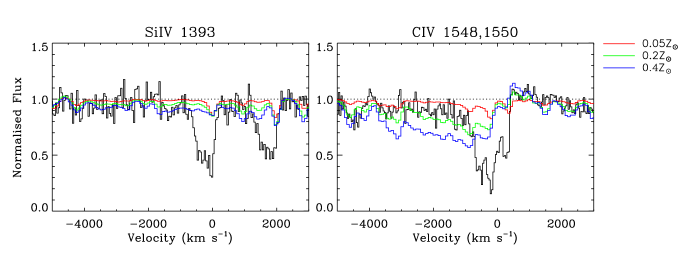
Figure 7: Velocity profiles of high-ionisation lines arising from the winds of massive stars. In each panel, the black histogram is the data for CSWA 20, plotted on a velocity scale relative to $z_{\rm sys}=1.433485$; the absorption features seen in these portions of the spectrum are blends of stellar and interstellar absorption lines. Superimposed on the data are theoretical stellar lines profiles for different metallicities computed with the Starburst99 spectral synthesis code and convolved to the same resolution as the data. In all three cases shown, we assumed continuous star formation, 100 Myr age, and a Salpeter IMF between 1 and 100 M_⊙. Further details are given in Section 5.3.

4.2.1 C/O abundance ratio

The correction we have applied to convert C²⁺/H⁺ to C/H assumes that C²⁺/O²⁺ = C/O. This may however not always be the case, given that both C⁺ and C²⁺ have lower ionisation potentials than O⁺ and O²⁺. This issue has recently been addressed by Erb et al. (2010) (see also Garnett et al. 1995; Shapley et al. 2003) with the aid of Cloudy photoionisation modelling. Erb et al. (2010) found that C²⁺/O²⁺ $\simeq$ C/O only for a relatively narrow range of values of the ionisation parameter, $U$, customarily defined as the ratio of the densities of ionising photons and particles. For the case in hand, we estimated the value of $U$ using the iterative equations of Kewley & Dopita (2002) together with the value of O/H derived for CSWA 20 and the [O iii] $\lambda 5008$/[O ii] $\lambda\lambda 3727,3729$ ratio. Interpolating between the 0.1 Z_⊙ and 0.2 Z_⊙ equations of Kewley & Dopita (2002) we find $\log U=-2.47\pm 0.09$ (the error quoted includes both the uncertainties in the measurements of the line fluxes and the difference between the 0.1 Z_⊙ and 0.2 Z_⊙ cases, added in quadrature). Inspection of Figure 11 of Erb et al. (2010) confirms that, in this range of values of $U$, C²⁺/O²⁺ is indeed a valid approximation to C/O.

As can be seen from Table 6, in CSWA 20 the carbon abundance relative to oxygen is significantly lower than in the Sun: $\log({\rm C/O})_{\rm CSWA\,20}=-1.06\pm 0.32$, between $\sim 1/3$ and $\sim 1/14$ of the solar value $\log({\rm C/O})_{\odot}=-0.26\pm 0.07$ (Asplund et al. 2009). This value is lower than measured in nearby dwarf galaxies of comparable oxygen abundance (e.g. Garnett et al. 1995), although still consistent within the errors. Christensen et al. (2012) also deduced $\log({\rm C/O})=-1.03\pm 0.08$ and $-0.80\pm 0.09$ in two high-$z$ gravitationally lensed galaxies with $12+\log{\rm(O/H)}=7.69\pm 0.13$ and $7.76\pm 0.03$ respectively, suggesting that an underabundance of C relative to O by one order of magnitude may not be unusual in such metal-poor environments.

There is continuing interest in measuring the C/O ratio at low metallicities (e.g. Akerman et al. 2004; Cooke et al. 2011) as a probe of stellar nucleosynthesis in this regime. The well-established decrease in C/O with decreasing O/H has been interpreted as evidence for metallicity-dependent yields of massive stars (Akerman et al. 2004) and/or delayed release of carbon into the ISM by stars of intermediate and low mass (e.g. Chiappini et al. 2003; Carigi et al. 2005). In Akerman et al. (2004) and Erb et al. (2010) it was pointed out that the similarity in the run of C/O vs. O/H between different locations and epochs in the Universe favoured the first explanation. Here we note that the lowest values of C/O measured in actively star-forming galaxies at high redshifts seem to be lower than the lowest measures of this ratio in Galactic halo stars (Akerman et al. 2004) by $\sim 0.4$ dex. Quite possibly, such a difference may simply reflect systematic offsets in the derivation of element abundances from stellar absorption spectra and H ii region emission spectra respectively. On the other hand, if the difference is real, it would suggest that both metallicity dependent yields and evolutionary effects (i.e. the past history of star formation), may determine the C/O ratio one would measure at a given oxygen abundance. In this scenario, the lowest values of C/O found in high-$z$ star-forming galaxies, such as CSWA 20, would reflect a particularly rapid progress of chemical evolution, with insufficient time for lower mass stars to evolve and contribute their carbon to the ISM.

5 Metallicity Indicators

As explained in the Introduction, one of the motivations for pursuing additional observations of CSWA 20 was the possibility of comparing different estimates of the metallicity thanks to the good match between the redshift of the galaxy and the wavelengths covered with the X-shooter spectrograph. The discussion in Section 3.1 demonstrates that, even with the aid of gravitational lensing, the detection of temperature sensitive auroral lines is often beyond the reach of current astronomical instrumentation. This has led to the development of approximate indicators of the oxygen abundance which use only strong nebular emission lines. We discuss two of these methods in Sections 5.1 and 5.2 respectively. In Sections 5.3 and 5.4 we consider two alternative estimates of the stellar metallicity based on the strengths of, respectively, the C iv (and Si iv) lines produced in the winds of the most luminous early-type stars, and a broad blend of Fe iii absorption lines near 1978 Å from the photospheres of B-type stars.

5.1 R₂₃ Index

The $R_{23}$ index first proposed by Pagel et al. (1979) is the most widely used approximate indicator of the oxygen abundance in star-forming galaxies being based on the ratios of what are typically the strongest emission lines from H ii regions at visible wavelengths: $R_{23}\equiv[I(3727)+I(3729)+I(4960)+I(5008)]/I$(H$\beta$). Its main drawback, in principle, is that the relationship between $R_{23}$ and O/H is double-valued, so that other line ratios may be required to break the degeneracy. Uncertainties in the reddening may also be an issue, given that the lines in question are spread over $\sim 1300$ Å of the optical spectrum. Regarding its application to high-redshift galaxies, however, the main difficulty encountered with ground-based observations is that all five emission lines fall within near-infrared atmospheric transmission windows only for a limited set of redshifts.

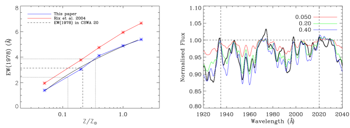
Figure 8: Left: Comparison of the old and new calibrations of the 1978 index, as indicated. The black line is the functional fit to the new calibration given in equation (3). Dashed and dotted lines show the value of the 1978 index measured in CSWA 20.  Right: Portion of the spectrum of CSWA 20 between 1920 and 2040 Å (smoothed to FWHM $=2.5$ Å, black line), together with synthetic Starburst99 spectra for three metallicities (coloured lines). The integration limits for the 1978 index are indicated by vertical dash lines. In both panels, all models are for 100 Myr old, continuous star formation with a Salpeter IMF. See Section 5.4 for further details.

At the redshift of CSWA 20, $z_{\rm sys}=1.433$, all the emission lines required to measure the $R_{23}$ index are free from strong water vapour absorption. In deducing O/H from the unreddened line fluxes in Table 4, we made use of the analytical expressions by McGaugh (1991) as given by Kobulnicky et al. (1999). These expression take into account the effect of the ionization parameter on the relationship between $R_{23}$ and O/H by including a term which depends on the ratio of the [O ii] and [O iii] lines, $O_{32}\equiv[I(4960)+I(5008)]/[I(3727)+I(3729)]$. We find 1$2+\log{\rm(O/H)}=7.96\pm 0.11$ and $8.59\pm 0.06$ for the low- and high-metallicity branches of the $R_{23}$ index respectively.

5.2 $N2$ Index

The $N2$ index (Denicoló et al. 2002; Pettini & Pagel 2004) has the advantage of involving only two emission lines at closely spaced wavelengths [$N2\equiv I(6585)/I$(H$\alpha$)], thereby avoiding the need to correct for extinction. On the other hand, it is only an approximate measure of O/H, with a precision of a factor of $\sim 2.5$ at the 95% confidence level (Pettini & Pagel 2004). Furthermore, the index saturates near solar metallicity. Nevertheless, it has had widespread application for galaxies at redshifts $z\lesssim 2.5$ (at higher redshifts the lines move beyond the atmospheric $K$-band window), thanks to its simplicity and convenience.

With the calibration by Pettini & Pagel (2004), the fluxes in Table 4 imply $12+\log{\rm(O/H)}=7.91\pm 0.09$ (where the uncertainty includes only the errors in the line fluxes). The same value is obtained with the more recent calibration of the $N2$ index by Marino et al. (2013). Thus, the $N2$ ratio identifies the lower-branch solution of the $R_{23}$ method as the one applicable to CSWA 20.

5.3 Stellar wind lines

The most prominent features in the rest-frame UV spectrum of CSWA 20 are absorption lines of C iv $\lambda\lambda 1548,1550$ and Si iv $\lambda\lambda 1393,1402$ (see Figures 2 and 5). These lines are blends of interstellar absorption and P-Cygni emission-absorption profiles from the winds of the most luminous OB stars in the galaxy. Over the last fifteen years, Claus Leitherer and collaborators have explored extensively how, in integrated galaxy spectra, the strength of the wind component of these lines depends on the age, initial mass function and metallicity of the stellar population (e.g. Leitherer 2011).

In the limiting case of continuous star formation at a constant rate with a universal IMF, the wind lines can be used as a metallicity indicator (e.g. Mehlert et al. 2002; Quider et al. 2010). Here, the ‘metallicity’ refers mostly to the abundances of C, N, O, and Fe, whose ions are the main contributors to the opacity driving the stellar winds (Vink et al. 2001). The attraction of this method is that it can applied at higher redshifts than the nebular emission line diagnostics (which, from the ground, are restricted to galaxies at $z\lesssim 3.8$); its limitations are the difficulty in separating stellar and interstellar absorption (Crowther et al. 2006), and the relatively coarse grid of stellar models currently available (Leitherer et al. 2010).

In Figure 7, we compare portions of the normalised spectrum of CSWA 20 with synthetic profiles generated by Starburst99 with the WM-basic library of theoretical stellar spectra (Leitherer et al. 2010). In generating the Starburst99 spectra, we assumed a Salpeter slope for the IMF between 1 and 100 M_⊙, continuous star formation at a constant rate over 100 Myr (at this age the UV spectrum has stabilised and no longer depends on the age of the starburst), and considered three metallicities of the OB stars: 0.05, 0.2 and 0.4 Z_⊙. The Starburst99 outputs were convolved to the resolution of our X-shooter spectrum (FWHM $\sim 0.9$ Å).

The left panel of Figure 7 shows that, at these metallicities, the Si iv stellar lines are very weak and of limited diagnostic value; the absorption we see is mostly interstellar. In the right panel, on the other hand, it is possible to distinguish the weak emission and broad, shallow blue wing of the stellar P-Cygni profile extending out to $\sim-4000$ km s^-1 from the narrower interstellar C iv absorption. The Starburst99 model with $Z=0.4$ Z_⊙ clearly overpredicts both emission and absorption components of the P-Cygni profile, whose overall strength is intermediate between those of the 0.2 Z_⊙ and 0.05 Z_⊙ models. We conclude that the metallicity of the most luminous OB stars in CSWA 20 is $Z_{\rm OB}\sim 0.1^{+0.1}_{-0.05}$ Z_⊙.

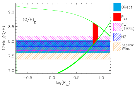
Figure 9: Comparison of different abundance indicators in CSWA 20. The green continuous lines show the upper and lower branch relations between the $R23$ index and the oxygen abundance (Section 5.1); the red vertical band connects the two solutions admitted by the $R23$ index measured in CSWA 20. The other methods are indicated by the colour key on the right. Note that although the $y$-axis indicates the abundance of oxygen, two of the methods [Stellar Wind and EW(1978)] measure a mix of elements [mostly Fe in the case of EW(19878)]. In plotting them here, we have assumed solar abundances relative to oxygen for the elements probed. The values shown graphically in the Figure are collected in Table 7.

Table 7: Summary of metallicity determinations^a.

Method	Element(s)	$Z/Z_{\odot}^{\rm b}$	Range of $Z/Z_{\odot}^{\rm c}$	Comments
$T_{\rm e}$	O	0.14	0.08–0.22	H ii regions
$R23$	O	0.19	0.14–0.24	H ii regions
$N2$	O	0.17	0.13–0.20	H ii regions
C iv	C, N, O, Fe	…	0.05–0.20	Stellar wind, O stars
1978	Fe	0.17	0.10–0.31	Photospheric, B stars

^a Solar abundances from Asplund et al. (2009).

^b Best fitting value of metallicity relative to solar (on a linear scale).

^c Range of metallicity relative to solar (on a linear scale).

5.4 The 1978 index

Between $\sim 1900$ and 2050 Å in the UV spectrum of a stellar population, there is a broad blend of Fe iii  lines formed in the photospheres of B-type stars. Rix et al. (2004) gave an account of the historical background to using this blend as an indicator of the Fe abundance. The main drawback in its application to high-$z$ galaxies is the shallow nature of this spectral feature, whose measured strength is therefore very sensitive to the exact placement of the continuum level.

We used the latest version of the Starburst99+WM-Basic models (Leitherer et al. 2010) to recalibrate the ‘1978 index’ (defined as the equivalent width between 1935 and 2020 Å) of Rix et al. (2004) who used an earlier version of the WM-Basic code (see Leitherer et al. 2010, for a description of the update). We followed the steps prescribed by Rix et al. (2004): we convolved the output spectra of Starburst99 (again for the case of 100 Myr old, continuous star formation with a Salpeter IMF) with a Gaussian of ${\rm FWHM}=2.5$ Å to match the resolution of most spectra of high-$z$ galaxies in the literature, and normalised the spectra by dividing by a spline fit to a set of pseudo-continuum points (Table 3 of Rix et al. 2004). The left panel of Figure 8 compares the new metallicity calibration of the 1978 index with the earlier one by Rix et al. (2004); the behaviour of the index is similar, but the new values are lower by $\sim 0.5$–1 Å for a given metallicity. The new dependence of EW(1978) on metallicity (essentially [Fe/H]) can be approximated by the quadratic relation:

$$\log\left(\frac{Z}{\hbox{Z${}_{\odot}$}}\right)=0.03x^{2}+0.17x-1.59$$ (3)

where $x=$ EW(1978) within the range 1.4–5.4 Å.

As can be seen from Figure 8 (right panel), the combination of the WM-basic libraries of theoretical stellar spectra and the Starburst99 spectral synthesis code is successful at reproducing the complex blend of photospheric absorption lines in this portion of the UV spectrum. Again, the observed spectrum of CSWA 20 appears to be intermediate between the 0.05 and 0.2 Z_⊙ cases. We measure EW(1978)${}_{\rm CSWA\,20}=3.1\pm 0.7$ Å; according to equation (3) this value corresponds to a metallicity $\log(Z_{\rm CSWA\,20}/Z_{\odot})=-0.76\pm 0.25$ ($Z_{\rm CSWA\,20}\simeq 1/3$–$1/10$ Z_⊙).

6 Discussion

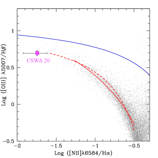
Figure 10: Zoom-in on a portion of the BPT diagram of Baldwin et al. (1981), showing the location of CSWA 20 (magenta point). The small grey points are galaxies from the Sloan Digital Sky Survey; the red curves are fits to the locus of local galaxies based on the relations by Maiolino et al. (2008) and Kewley & Ellison (2008). The blue continuous line divides star-forming galaxies from Active Galactic Nuclei according to the models by Kewley et al. (2001).

In Table 7 and Figure 9 we bring together the different determinations of metallicity in CSWA 20 discussed in Sections 4 and 5. Evidently, in this galaxy all five methods give consistent values of the metallicity. The agreement between the ‘direct’ method, based on detecting weak auroral lines, and the more approximate strong-line indices $R23$ and $N2$ is encouraging. On the other hand, and perhaps counterintuitively, the apparent good match between the abundance of O in the H ii regions of CSWA 20 and that of Fe in the photospheres of its early-type stars may be less reassuring. In Section 4.2.1 it was suggested that the unusually low C/O ratio may be related to a rapid timescale of chemical enrichment, with the release of C into the ISM somewhat delayed relative to that of O. If this explanation is correct, then one may also have expected a subsolar Fe/O ratio, by a factor of $\sim 2$–3. Quite possibly, such a degree of $\alpha$-element enhancement is hidden in the uncertainties associated with the calibration and use of stellar metallicity indicators. It may well be premature to try and discern such subtleties in the chemical composition of high-$z$ galaxies, given the limitations of current models and data.

Returning to the nebular emission lines, it is now well established that high-$z$ star-forming galaxies are clearly separated from local counterparts when their emission line ratios are plotted on the plane [O iii]/H$\beta$–[N ii]/H$\alpha$, commonly referred to as the ‘BPT’ diagram of Baldwin et al. (1981). The recent work by Steidel et al. (in preparation) provides a vivid demonstration of the shift to higher values of [O iii]/H$\beta$ for a given [N ii]/H$\alpha$ (and vice versa) found in galaxies at $z\sim 2.3$, compared to the bulk of star-forming galaxies in the nearby Universe (see also Brinchmann et al. 2008; Liu et al. 2008; Masters et al. 2014, and references therein). Such a shift has been interpreted as the result of more extreme conditions (higher densities, more intense and harder radiation fields) in the H ii regions of the luminous high-$z$ galaxies targeted by existing surveys (e.g. Kewley et al. 2013).

It is reasonable to question, therefore, whether calibrations of the strong-line indices developed from samples of nearby galaxies can be applied in the high-redshift Universe, and what systematic errors they may introduce in the abundances so derived. As can be seen from Figure 10, CSWA 20 lies near the top-left corner of the BPT diagram, at log([O iii]/H$\beta$), log([N ii]/H$\alpha$) $=+0.69,-1.75$, a locus occupied by few galaxies at all redshifts (its weak [N ii] lines are below the detection limits of most large surveys). Nevertheless, it does appear to lie on an extrapolation to low metallicity of the mean relation for local galaxies. Thus, it may not be surprising that all three measures of the oxygen abundance in Table 7 are in good mutual agreement, and we gain little guidance from CSWA 20 in assessing the systematic errors which may affect the application of the strong-line indices to other star-forming galaxies at $z=2$–3.

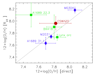
Figure 11: Comparison between the oxygen abundance deduced from auroral lines (the ‘direct’ method) and from the strong-line index $R23$ in the few high-$z$ star-forming galaxies where both measures are available from the literature. The blue diamonds are from the work by Christensen et al. (2012). The green squares are from Yuan & Kewley (2009, A1689 22.3), Erb et al. (2010, BX418), and Villar-Martín et al. (2004, Lynx arc), respectively. $1\sigma$ uncertainties are indicated by the error bars.

To explore this point further, we compare in Figure 11 the oxygen abundance deduced with the $T_{\rm e}$ and $R23$ methods in the few high-$z$ star-forming galaxies where both values have been reported in the literature. Evidently, within the limitations of this very small sample, CSWA 20 is not unique in showing a reasonable agreement between the two approaches, with the only deviant point being the $z=1.705$ galaxy 22.3 behind the cluster Abell 1689 observed by Yuan & Kewley (2009). Future near-IR observations of much larger samples of $z\simeq 1.5$–3 star-forming galaxies, now made possible by the advent of the MOSFIRE spectrograph (McLean et al. 2010), will undoubtedly help us assess better the validity of different nebular abundance measures in the high-$z$ galaxy population.

7 Summary

In this paper, we have analysed VLT+X-shooter observations of CSWA 20, a $z=1.433$ star-forming galaxy whose apparent magnitude is boosted by a factor of 11.5 ($-2.7$ mag) by gravitational lensing by a foreground massive elliptical galaxy at $z=0.741$. The boost provided by the lens gives us access to weaker spectral features and allows us to record the spectrum at higher resolution than is normally the case; coupled with the wide wavelength coverage of X-shooter, all these factors give us an in-depth view of the physical conditions in a galaxy which was actively forming stars $\sim 9$ Gyr ago. The main results of this work are as follows.

1. CSWA 20 has a metallicity $Z\sim 1/7$ Z_⊙, measured from its H ii regions and massive stars. Its current star-formation rate is $\sim$6 M_⊙ yr^-1, one order of magnitude lower than the star formation rate of $L^{\ast}$ galaxies at $z\sim 2$ (Reddy et al. 2008). The sub-solar metallicity is reflected in the high temperature of its H ii regions, $T_{\rm e}$ $\simeq 17000$ K, compared to $T_{\rm e}$ $\simeq 10000$ K typical of H ii regions in nearby galaxies.

2. Carbon is significantly less abundant than oxygen, compared to the solar ratio of of these two elements. The value we find, $\log{\rm C/O}=-1.06\pm 0.32$, is among the lowest measured in metal-poor H ii galaxies, and $\sim 2$–3 times lower than in Galactic halo stars of similar oxygen abundance. Possibly, chemical enrichment has proceeded at such a rapid rate in CSWA 20 that the low and intermediate mass stars which contribute some of the carbon have not had sufficient time yet to catch up with the prompt release of oxygen from more massive stars.

3. With our data, we can use five different methods to measure the metallicity of the galaxy; three are based on emission lines from H ii regions and two on absorption features in the atmospheres of massive stars. All five routes give the same value of metallicity within a factor of $\sim 2$. Of the three determinations of the oxygen abundance from emission lines, one uses the density and temperature of the H ii regions, while the other two rely on approximate local calibrations of strong line ratios. In CSWA 20, all three methods give the same answer, but this may not be surprising, given that this galaxy falls on an extrapolation to low metallicity of the locus occupied by local galaxies in the BPT diagnostic diagram.

4. In the course of the analysis performed here, we have recalibrated the dependence on metallicity of the Fe iii 1978 index of Rix et al. (2004), using the latest combination of the Starburst99 spectral synthesis code and the WM-basic suite of theoretical stellar spectra.

5. Most interstellar absorption lines are unusually weak in CSWA 20, probably as a result of a very patchy coverage of the starburst by the ISM, as viewed from our direction. The resolved kinematics of the absorption reveal gas spread over nearly 1000 km ^-1, with most of the absorption taking place in gas which is outflowing from the galaxy with velocities of up to $\sim 750$ km s^-1. The maximum speed reached by the outflow is similar to the values measured in a few other gravitationally lensed galaxies at $z\sim 1.5$–3, despite the order-of-magnitude difference in the star-formation rates among these galaxies. Thus it is unclear to what extent the terminal velocity of the ‘superwind’ in galaxies with high star-formation rate surface densities depends on the total energy and momentum deposited into the ISM by the central starburst.

All in all, our observations of CSWA 20 have left us with many questions, as well as providing some answers. While it is generally appreciated that physical conditions in the galaxies responsible for the bulk of the star formation activity at earlier epochs are markedly different from those encountered in the local Universe, we still lack a proper physical framework that can help us put into context the results of studies such as the one presented here. A major limiting factor at present is the paucity of high redshift galaxies bright enough to be studied in detail, so that correlations between age, mass, star-formation history, metallicity, and large-scale outflows in the ISM can be explored. Undoubtedly, future observations of other gravitationally lensed galaxies will in time fill in the many gaps that still remain.

8 Acknowledgements

We are grateful to the European Southern Observatory time assignment committee who awarded time to this programme, and to the staff astronomers at Paranal who conducted the observations. It is a pleasure to acknowledge the help by Sergey Koposov with various aspects of the data analysis. Vasily Belokurov kindly provided the WHT images of CSWA 20 reproduced in Figure 1, and Naveen Reddy the composite of BM galaxy spectra used in Figure 5. We are also grateful to Mike Barlow, Claus Leitherer and Daniela Calzetti for useful discussions, and to the anonymous referee whose comments and suggestions improved the paper. . LC is supported by the European Union under a Marie Curie Intra-European fellowship, contract PIEF-GA-2010-274117.

References

- Akerman et al. (2004) Akerman C. J., Carigi L., Nissen P. E., Pettini M., Asplund M., 2004, A&A, 414, 931
- Asplund et al. (2009) Asplund M., Grevesse N., Sauval A. J., Scott P., 2009, ArA&A, 47, 481
- Auger et al. (2013) Auger M. W., Budzynski J. M., Belokurov V., Koposov S. E., McCarthy I., 2013, ArXiv e-prints
- Baldwin et al. (1981) Baldwin J. A., Phillips M. M., Terlevich R., 1981, PASP, 93, 5
- Bayliss et al. (2014) Bayliss M. B., Rigby, J. R., Sharon, K., et al., 2014, ApJ, in press (arXiv:1310.6695)
- Becker et al. (2009) Becker G. D., Rauch M., Sargent W. L. W., 2009, ApJ, 698, 1010
- Belokurov et al. (2009) Belokurov V., Evans N. W., Hewett P. C., Moiseev A., McMahon R. G., Sanchez S. F., King L. J., 2009, MNRAS, 392, 104
- Brinchmann et al. (2008) Brinchmann J., Pettini M., Charlot S., 2008, MNRAS, 385, 769
- Brocklehurst (1971) Brocklehurst M., 1971, MNRAS, 153, 471
- Calzetti et al. (2000) Calzetti D., Armus L., Bohlin R. C., Kinney A. L., Koornneef J., Storchi-Bergmann T., 2000, ApJ, 533, 682
- Carigi et al. (2005) Carigi L., Peimbert M., Esteban C., García-Rojas J., 2005, ApJ, 623, 213
- Chabrier (2003) Chabrier G., 2003, PASP, 115, 763
- Chiappini et al. (2003) Chiappini C., Romano D., Matteucci F., 2003, MNRAS, 339, 63
- Christensen et al. (2012) Christensen L., Laursen P., Richard J., Hjorth J., Milvang-Jensen B., Dessauges-Zavadsky M., Limousin M., Grillo C., Ebeling H., 2012, MNRAS, 427, 1973
- Cooke et al. (2011) Cooke R., Pettini M., Steidel C. C., Rudie G. C., Nissen P. E., 2011, MNRAS, 417, 1534
- Crowther et al. (2006) Crowther P. A., Prinja R. K., Pettini M., Steidel C. C., 2006, MNRAS, 368, 895
- Denicoló et al. (2002) Denicoló G., Terlevich R., Terlevich E., 2002, MNRAS, 330, 69
- Dessauges-Zavadsky et al. (2010) Dessauges-Zavadsky M., D’Odorico S., Schaerer D., Modigliani A., Tapken C., Vernet J., 2010, A&A, 510, A26
- Erb et al. (2010) Erb D. K., Pettini M., Shapley A. E., Steidel C. C., Law D. R., Reddy N. A., 2010, ApJ, 719, 1168
- Erb et al. (2006a) Erb D. K., Shapley A. E., Pettini M., Steidel C. C., Reddy N. A., Adelberger K. L., 2006a, ApJ, 644, 813
- Erb et al. (2006b) Erb D. K., Steidel C. C., Shapley A. E., Pettini M., Reddy N. A., Adelberger K. L., 2006b, ApJ, 647, 128
- Fitzpatrick (1999) Fitzpatrick, E. L. 1999, PASP, 111, 63
- Garnett et al. (1995) Garnett D. R., Skillman E. D., Dufour R. J., Peimbert M., Torres-Peimbert S., Terlevich R., Terlevich E., Shields G. A., 1995, ApJ, 443, 64
- Hainline et al. (2009) Hainline K. N., Shapley A. E., Kornei K. A., Pettini M., Buckley-Geer E., Allam S. S., Tucker D. L., 2009, ApJ, 701, 52
- Halliday et al. (2008) Halliday C., Daddi E., Cimatti A., Kurk J., Renzini A., Mignoli M., Bolzonella M., Pozzetti L., Dickinson M., Zamorani G., Berta S., Franceschini A., Cassata P., Rodighiero G., Rosati P., 2008, A&A, 479, 417
- Heckman (2002) Heckman T. M., 2002, in Astronomical Society of the Pacific Conference Series, Vol. 254, Extragalactic Gas at Low Redshift, Mulchaey J. S., Stocke J. T., eds., p. 292
- Henry et al. (2000) Henry R. B. C., Edmunds M. G., Köppen J., 2000, ApJ, 541, 660
- Izotov et al. (2006) Izotov Y. I., Stasińska G., Meynet G., Guseva N. G., Thuan T. X., 2006, A&A, 448, 955
- Kelson (2003) Kelson D. D., 2003, PASP, 115, 688
- Kewley & Dopita (2002) Kewley L. J., Dopita M. A., 2002, ApJS, 142, 35
- Kewley et al. (2013) Kewley L. J., Dopita M. A., Leitherer C., Davé R., Yuan T., Allen M., Groves B., Sutherland R., 2013, ApJ, 774, 100
- Kewley et al. (2001) Kewley L. J., Dopita M. A., Sutherland R. S., Heisler C. A., Trevena J., 2001, ApJ, 556, 121
- Kewley & Ellison (2008) Kewley L. J., Ellison S. L., 2008, ApJ, 681, 1183
- Kingsburgh & Barlow (1994) Kingsburgh R. L., Barlow M. J., 1994, MNRAS, 271, 257
- Kobulnicky et al. (1999) Kobulnicky H. A., Kennicutt Jr. R. C., Pizagno J. L., 1999, ApJ, 514, 544
- Kornei et al. (2013) Kornei K. A., Shapley A. E., Martin C. L., Coil A. L., Lotz J. M., Weiner B. J., 2013, ArXiv e-prints
- Kubo et al. (2009) Kubo J. M., Allam S. S., Annis J., Buckley-Geer E. J., Diehl H. T., Kubik D., Lin H., Tucker D., 2009, ApJL, 696, L61
- Leitherer (2011) Leitherer C., 2011, in Astronomical Society of the Pacific Conference Series, Vol. 440, UP2010: Have Observations Revealed a Variable Upper End of the Initial Mass Function?, Treyer M., Wyder T., Neill J., Seibert M., Lee J., eds., p. 309
- Leitherer et al. (2010) Leitherer C., Ortiz Otálvaro P. A., Bresolin F., Kudritzki R.-P., Lo Faro B., Pauldrach A. W. A., Pettini M., Rix S. A., 2010, ApJS, 189, 309
- Liu et al. (2008) Liu X., Shapley A. E., Coil A. L., Brinchmann J., Ma C.-P., 2008, ApJ, 678, 758
- Madau & Dickinson (2014) Madau P., Dickinson M., 2014, ARAA, in press
- Maiolino et al. (2008) Maiolino R., Nagao T., Grazian A., Cocchia F., Marconi A., Mannucci F., Cimatti A., Pipino A., Ballero S., Calura F., Chiappini C., Fontana A., Granato G. L., Matteucci F., Pastorini G., Pentericci L., Risaliti G., Salvati M., Silva L., 2008, A&A, 488, 463
- Maraston et al. (2009) Maraston C., Nieves Colmenárez L., Bender R., Thomas D., 2009, A&A, 493, 425
- Marino et al. (2013) Marino R. A., Rosales-Ortega F. F., Sánchez S. F., Gil de Paz A., Vílchez J., Miralles-Caballero D., Kehrig C., Pérez-Montero E., Stanishev V., Iglesias-Páramo J., Díaz A. I., Castillo-Morales A., Kennicutt R., López-Sánchez A. R., Galbany L., García-Benito R., Mast D., Mendez-Abreu J., Monreal-Ibero A., Husemann B., Walcher C. J., García-Lorenzo B., Masegosa J., del Olmo Orozco A., Mourão A. M., Ziegler B., Mollá M., Papaderos P., Sánchez-Blázquez P., González Delgado R. M., Falcón-Barroso J., Roth M. M., van de Ven G., the CALIFA team, 2013, ArXiv e-prints
- Martin et al. (2012) Martin C. L., Shapley A. E., Coil A. L., Kornei K. A., Bundy K., Weiner B. J., Noeske K. G., Schiminovich D., 2012, ApJ, 760, 127
- Masters et al. (2014) Masters, D., McCarthy, P., Siana, B., et al. 2014, arXiv:1402.0510
- McGaugh (1991) McGaugh S. S., 1991, ApJ, 380, 140
- McLean et al. (2010) McLean I. S., Steidel C. C., Epps H., Matthews K., Adkins S., Konidaris N., Weber B., Aliado T., Brims G., Canfield J., Cromer J., Fucik J., Kulas K., Mace G., Magnone K., Rodriguez H., Wang E., Weiss J., 2010, in Society of Photo-Optical Instrumentation Engineers (SPIE) Conference Series, Vol. 7735, Society of Photo-Optical Instrumentation Engineers (SPIE) Conference Series
- Mehlert et al. (2002) Mehlert D., Noll S., Appenzeller I., Saglia R. P., Bender R., Böhm A., Drory N., Fricke K., Gabasch A., Heidt J., Hopp U., Jäger K., Möllenhoff C., Seitz S., Stahl O., Ziegler B., 2002, A&A, 393, 809
- Morton (2003) Morton D. C., 2003, ApJS, 149, 205
- Pagel et al. (1979) Pagel B. E. J., Edmunds M. G., Blackwell D. E., Chun M. S., Smith G., 1979, MNRAS, 189, 95
- Pettini (2006) Pettini M., 2006, in The Fabulous Destiny of Galaxies: Bridging Past and Present, Le Brun V., Mazure A., Arnouts S., Burgarella D., eds., p. 319
- Pettini et al. (2010) Pettini M., Christensen L., D’Odorico S., Belokurov V., Evans N. W., Hewett P. C., Koposov S., Mason E., Vernet J., 2010, MNRAS, 402, 2335
- Pettini & Pagel (2004) Pettini M., Pagel B. E. J., 2004, MNRAS, 348, L59
- Pettini et al. (2002) Pettini M., Rix S. A., Steidel C. C., Adelberger K. L., Hunt M. P., Shapley A. E., 2002, ApJ, 569, 742
- Pettini et al. (2001) Pettini M., Shapley A. E., Steidel C. C., Cuby J.-G., Dickinson M., Moorwood A. F. M., Adelberger K. L., Giavalisco M., 2001, ApJ, 554, 981
- Pettini et al. (2000) Pettini M., Steidel C. C., Adelberger K. L., Dickinson M., Giavalisco M., 2000, ApJ, 528, 96
- Pettini et al. (2008) Pettini M., Zych B. J., Steidel C. C., Chaffee F. H., 2008, MNRAS, 385, 2011
- Quider et al. (2009) Quider A. M., Pettini M., Shapley A. E., Steidel C. C., 2009, MNRAS, 398, 1263
- Quider et al. (2010) Quider A. M., Shapley A. E., Pettini M., Steidel C. C., Stark D. P., 2010, MNRAS, 402, 1467
- Reddy et al. (2008) Reddy N. A., Steidel C. C., Pettini M., Adelberger K. L., Shapley A. E., Erb D. K., Dickinson M., 2008, ApJS, 175, 48
- Richard et al. (2011) Richard J., Jones T., Ellis R., Stark D. P., Livermore R., Swinbank M., 2011, MNRAS, 413, 643
- Rigby et al. (2011) Rigby J. R., Wuyts E., Gladders M. D., Sharon K., Becker G. D., 2011, ApJ, 732, 59
- Rix et al. (2004) Rix S. A., Pettini M., Leitherer C., Bresolin F., Kudritzki R.-P., Steidel C. C., 2004, ApJ, 615, 98
- Rubin et al. (2010) Rubin K. H. R., Weiner B. J., Koo D. C., Martin C. L., Prochaska J. X., Coil A. L., Newman J. A., 2010, ApJ, 719, 1503
- Shapley et al. (2003) Shapley A. E., Steidel C. C., Pettini M., Adelberger K. L., 2003, ApJ, 588, 65
- Sommariva et al. (2012) Sommariva V., Mannucci F., Cresci G., Maiolino R., Marconi A., Nagao T., Baroni A., Grazian A., 2012, A&A, 539, A136
- Stark et al. (2013) Stark D. P., Auger M., Belokurov V., Jones T., Robertson B. E., Ellis R. S., Sand D. J., Moiseev A., Eagle W., Myers T., 2013, ArXiv e-prints
- Stasinska (2005) Stasińska G., 2005, A&A, 434, 507
- Steidel et al. (2010) Steidel C. C., Erb D. K., Shapley A. E., Pettini M., Reddy N., Bogosavljević M., Rudie G. C., Rakic O., 2010, ApJ, 717, 289
- Steidel et al. (2004) Steidel C. C., Shapley A. E., Pettini M., Adelberger K. L., Erb D. K., Reddy N. A., Hunt M. P., 2004, ApJ, 604, 534
- Vernet et al. (2011) Vernet J., Dekker H., D’Odorico S., Kaper L., Kjaergaard P.,, 2011, A&A, 536, A105
- Villar-Martín et al. (2004) Villar-Martín M., Cerviño M., González Delgado R. M., 2004, MNRAS, 355, 1132
- Vink et al. (2001) Vink J. S., de Koter A., Lamers H. J. G. L. M., 2001, A&A, 369, 574
- Yuan & Kewley (2009) Yuan T.-T., Kewley L. J., 2009, ApJL, 699, L161