Characterization of an in-vacuum PILATUS 1M detector

Abstract

A dedicated in-vacuum X-ray detector based on the hybrid pixel PILATUS 1M detector has been installed at the four-crystal monochromator beamline of PTB at the electron storage ring BESSY II in Berlin. Due to its windowless operation, the detector can be used in the entire photon energy range of the beamline from 10 keV down to 1.75 keV for small-angle X-ray scattering (SAXS) experiments and anomalous SAXS (ASAXS) at absorption edges of light elements. The radiometric and geometric properties of the detector like quantum efficiency, pixel pitch and module alignment have been determined with low uncertainties. The first grazing incidence SAXS (GISAXS) results demonstrate the superior resolution in momentum transfer achievable at low photon energies.

I Introduction

The advances of integrated circuits in the last few decades have significantly boosted the development of X-ray detectors Yaffe and Rowlands (1997). So-called hybrid pixel X-ray detectors have been developed, which consist of a readout chip bump bonded on a silicon sensor that acts as a radiation absorber Heijne and Jarron (1989). State-of-the-art detectors like the XPAD Delpierre et al. (2007), detectors based on the Medipix readout chip Ponchut et al. (2002); Pennicard et al. (2010), and the PILATUS Broennimann et al. (2006); Kraft et al. (2009a) combine a semiconductor pixel matrix with a readout chip providing an amplifier, comparator and digital counter for every single pixel. This is appealing especially for scattering and diffraction experiments, where the photon flux at individual pixels may vary over many orders of magnitude. As opposed to dose-proportional detectors, photon counting can provide very low darkcount rates, and consequently huge dynamic ranges, signal-to-noise ratios close to the quantum limit and negligible crosstalk between neighbouring pixels resulting in a nearly perfect point spread function Chmeissani et al. (2004).

The commercially available large-area (1 megapixel and above) hybrid pixel detectors are operated in air and the radiation enters through a thin window. This window limits the detectable photon energy range to energies above approximately $5~{}\mathrm{keV}$ due to absorption in the window. Yet the absorption edges of technologically and biologically relevant elements like silicon, phosphorus, sulphur, chlorine, or calcium are situated below this energy. To overcome this limitation, windowless operation in vacuum with a direct connection to the sample chamber is necessary. The suitability and performance of a PILATUS 100k detector under such conditions has been shown previously Marchal and Wagner (2011); Marchal et al. (2011). Moreover, extensive testing and characterization of detector modules in vacuum Donath et al. (2013) has been carried out in collaboration with Dectris Ltd. at the four-crystal monochromator (FCM) beamline in the laboratory of the Physikalisch-Technische Bundesanstalt (PTB) at the electron storage ring BESSY II. However, these setups were preliminary experiments with a single module as a proof of concept at that time, a fully operational multi-module large-area in-vacuum PILATUS has not been realized up to now.

In this paper, we fill this gap and describe the modifications made to the PILATUS 1M modular detector in collaboration with Dectris Ltd. to operate under vacuum, so that the experimentally accessible energy range is widened downwards to a photon energy $E_{\textrm{\small\scriptsize ph}}$ of $1.75~{}\mathrm{keV}$. Radiometric as well as geometric characterization has been performed using traceable methods. The first measurement results in a typical scattering setup are reported to demonstrate the extended measurement capabilities at X-ray photon energies below $4~{}\mathrm{keV}$.

II Experimental setup

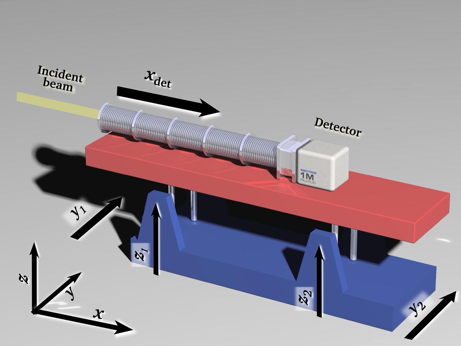
Figure 1: Motor axes of the SAXS setup. The axes for longitudinal detector movement $x_{\mathrm{det}}$ and for vertical movement of the stage $z_{1}$ and $z_{2}$ are equipped with optical encoders for absolute length measurements with micrometer resolution.

The in-vacuum PILATUS 1M detector was specifically developed and scaled to the parameters of the small-angle scattering setup of the FCM beamline Krumrey et al. (2011); Beckhoff et al. (2009). The beamline Krumrey and Ulm (2001) covers a photon energy range of $1.75~{}\mathrm{keV}$ to $10~{}\mathrm{keV}$, which defines the targeted lower energy limit of the detector. The monochromator features an energy resolving power $E_{\textrm{\small\scriptsize ph}}/\Delta E_{\textrm{\small\scriptsize ph}}$ of $10^{4}$ and an accuracy of the energy scale of 0.5 eV Krumrey and Ulm (2001); Krumrey (1998). The photon flux of the incident beam at the location of the sample or detector can be measured in a traceable way by photodiodes that were calibrated against a cryogenic electric substitution radiometer Gerlach et al. (2008) within a relative uncertainty of $1\ \%$. A sample chamber equipped with six axes for sample movement is attached to the FCM beamline Fuchs et al. (1995). For small-angle X-ray scattering measurements in transmission geometry (i.e., SAXS) and grazing-incidence reflection geometry (i.e., GISAXS), the 2D-detector is usually mounted on the SAXS instrument of the Helmholtz-Zentrum Berlin (HZB) Hoell et al. (2007) as illustrated in Figure 1. The detector is installed on a moveable stage (to the rear of Figure 1) and connected to an edge-welded bellow to allow any sample-to-detector distance between $1.75\ \mathrm{m}$ and about $4.5\ \mathrm{m}$, and a vertical tilt angle up to 3° without breaking the vacuum. The translation axes $z_{1}$, $z_{2}$, and $x_{\mathrm{det}}$ are equipped with optical encoders (Heidenhain AE LC 182 and AE LC 483) which measure the displacement on an absolute scale with an accuracy of 1 µm. These encoders establish the traceability of the detector displacement. The detector side of the bellow holds a moveable beamstop to block the intense transmitted or specularly reflected fraction of the beam.

III Technical implementation of the in-vacuum version

Table 1: Technical specifications of the in-vacuum PILATUS 1M detector.

parameter	value / setting
accessible photon energy	$1.75~{}\mathrm{keV}$ …$>36~{}\mathrm{keV}$
sensitive detector area	179 mm $\times$ 169 mm
sensor thickness	320 µm
dimensions	ca. 60 cm $\times$ 37 cm $\times$ 37 cm
mass	ca. 80 kg
entrance flange	DN 250 CF
typical cooler temperature	5 °C …10 °C
typical operation pressure	$<1\times 10^{-5}$ mbar
pressure gauge	Pfeiffer PKR 251

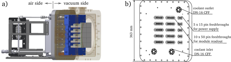
Figure 2: (a) Sketch of the vacuum-compatible version of the PILATUS detector. The vacuum side (on the right) consists of the ten detector modules (grey) mounted on the downsized module carrier plate (blue). This is attached to the feed-through flange plate that contains the 575 electric connections and the water supply lines. The vacuum chamber (semi-transparent structure) is directly connected to the beamline. The air side (on the left) consists of the standard electronic units of the PILATUS and the water cooling supply. (b) Sketch of the feed-through flange plate that separates the vacuum and the air side and facilitates the electrical connection of detector modules.

One of the design goals for a vacuum-compatible version of the PILATUS 1M detector was to minimize the number of modifications from the standard detector. The final solution was a vacuum-proof separation of the detector modules from the electronic control units. To this end, a vacuum chamber for the modules and a feed-through flange plate were developed. The ten detector modules are mounted on a size-reduced module carrier plate. The carrier plate is connected to the feed-through flange plate which closes the vacuum chamber at the detector side. Figure 2a shows a sketch of the general setup.

The vacuum chamber encloses the detector modules that provide a total sensitive area of 179 mm $\times$ 169 mm with a sensor thickness of 320 µm. The CF-entrance flange has a diameter of 250 mm to prevent any shadowing of the detector surface and is directly connected to the HZB SAXS instrument. A vacuum gauge is used for pressure monitoring and controls an interlock system, which shuts down the high voltage of the detector in case of vacuum loss. The feed-through flange plate, Figure 2b, seals the vacuum chamber on the opposite side and facilitates the connection of the 575 electric lines and the channels for water cooling. On the air side, standard PILATUS 1M electronic units are used for data processing. The module carrier plate is cooled with circulating water kept at a constant temperature of typically 5 °C. Table 1 gives an overview of the technical specifications of the in-vacuum PILATUS 1M detector. Operation in air at higher photon energies is still possible with the modified PILATUS 1M setup. To this end, a Mylar window is attached to the entrance flange of the vacuum chamber.

Before we describe the necessary electronic adjustments, the operation principle of the PILATUS hybrid pixel detector needs to be reviewed briefly. Many more details can be found in Broennimann et al. (2006); Kraft et al. (2009a, b). The detection principle in each pixel is based on the generation of electron-hole pairs in a silicon pn-junction induced by an absorbed X-ray photon. The electric charge is amplified by a charge-sensitive preamplifier (CSA), the amplification of which can be set in discrete steps, which are called the gain modes Kraft et al. (2009b). The amplified pulse is then compared to an adjustable threshold voltage $V_{\textrm{\scriptsize thresh}}$ by a comparator. The pulse is registered and counted only if it exceeds the threshold, and otherwise discarded. The voltage threshold $V_{\textrm{\scriptsize thresh}}$ corresponding to a photon energy threshold $E_{\textrm{\scriptsize thresh}}$ is determined by the software depending on the amplifier gain. In normal operation mode, the energy threshold $E_{\textrm{\scriptsize thresh}}$ is set to $\frac{1}{2}\ E_{\textrm{\small\scriptsize ph}}$ to avoid charge-sharing counts in neighbouring pixels Chmeissani et al. (2004).

For the in-vacuum PILATUS 1M detector, an additional ultra-high gain mode with higher amplification than the standard high-gain mode was added to account for the reduced number of electron-hole pairs generated by each photon at low X-ray photon energy. The lowest achievable $E_{\textrm{\scriptsize thresh}}$ is ultimately limited by amplifier noise exceeding the comparator threshold $V_{\textrm{\scriptsize thresh}}$  or by the onset of instable operation. The minimum threshold determined is $E_{\textrm{\scriptsize thresh}}=1.7~{}\mathrm{keV}$ for stable operation in ultra-high gain mode. For the preferred threshold setting with $E_{\textrm{\scriptsize thresh}}=\frac{1}{2}\ E_{\textrm{\small\scriptsize ph}}$, this would only allow a minimal photon energy of $3.4~{}\mathrm{keV}$. In order to reach lower photon energies, for example, the silicon absorption K-edge at $1.84~{}\mathrm{keV}$, $E_{\textrm{\scriptsize thresh}}$ can be set independently of the photon energy to a higher level. This results in a decreased count rate, but it also leads to a smaller effective pixel area because only photons that deposit at least a fraction of $E_{\textrm{\scriptsize thresh}}/E_{\textrm{\small\scriptsize ph}}$ of their energy in the pixel contribute to the counts Schubert et al. (2010). As a result, undersampling and aliasing occur which might even be an advantageous effect in some experiments, where a refined detector point spread function is needed Farsiu et al. (2004). However, the usage of the ultra-high gain mode results in an increased detector dead-time of about 4 µs, which results in a loss of registered photons Marchal and Wagner (2011).

IV Radiometric characterization

The quantum efficiency ($\mathit{QE}$) of the detector, which is the ratio of registered counts to incident photons, was determined as a basis for measurements of absolute scattering intensities. The $\mathit{QE}$ measurements were accomplished by taking sequences of images of the monochromatized synchrotron beam with varying energy. Before and after each sequence, the incident photon flux at each energy was determined by a calibrated photodiode. The monochromatic photon flux of the beamline is in the order of $10^{9}\ \mathrm{s^{-1}}$ to $10^{10}\ \mathrm{s^{-1}}$ in an area of about $0.5\ \mathrm{mm^{2}}$ at the usual top-up ring current of $300\ \mathrm{mA}$ of the storage ring. This photon flux is well beyond the linear, unsaturated, detector response range, in particular in ultra-high gain mode and at low threshold energies. Hence, BESSY II was operated in a special mode where the ring current was reduced stepwise to 832 µA, 409 µA, 95 µA, and finally 6 µA. This also allowed us to evaluate the linearity of the registered count rate in relation to the rate of incoming photons. The $\mathit{QE}$ was determined from the measurements at the lowest ring current, which resulted in photocurrents of the calibrated diodes from $14~{}\mathrm{pA}$ to $1.2~{}\mathrm{nA}$ (darkcurrent $<1~{}\mathrm{pA}$). Additionally, the beam was defocused so that the most intense spot covered an area of approximately 100 pixels. In this way, the maximum flux of incoming photons and pixel was kept below 20 000 $\mathrm{s}^{-1}$, while the minimum photon flux in the evaluated region of 10 $\mathrm{s}^{-1}$ still exceeded the darkcount rate of $10^{-5}\ \mathrm{s}^{-1}$ by several orders of magnitude.

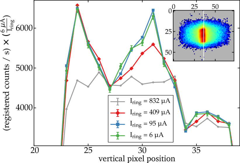
Figure 3: Registered counts per second along the most intense region of the illuminated area (see inset for a logarithmic image of the spot shape, the white line indicates the cut line of the plotted profiles). The detector images where recorded at four different storage ring currents under otherwise identical conditions ($E_{\textrm{\small\scriptsize ph}}$= $2.5~{}\mathrm{keV}$). Each profile has been scaled by the ratio of minimal ring current (6 µA) and the ring current of the profile. Deviations from a linear counting behaviour manifest in lower scaled count rate in comparison to the 6 µA profile.

Before the $\mathit{QE}$ can be accurately determined, the linear response of the detector must be checked and the uncertainty contributions need to be evaluated. Displayed in Figure 3 are the registered counts per second and per pixel along the most intense line of the illuminated area (see vertical line in the inset) for the four different ring currents, each recorded under otherwise identical conditions at $E_{\textrm{\small\scriptsize ph}}=2.5~{}\mathrm{keV}$. The profiles have been scaled by the ratio of the ring current of the $\mathit{QE}$ measurements (6 µA) to the corresponding ring current of the profile. In this way, an increase of detector saturation due to a too high rate of incoming photons (which is equivalent to the ring current) can be observed by a deviation from the unscaled count rate profile measured at 6 µA. It can be seen that the profiles of 832 µA and 409 µA deviate significantly from the 6 µA profile, clearly indicating the occurrence of saturation. But the profile of 95 µA differs by less than 2.2 % from the 6 µA data, which should give an upper estimate for the increase of saturation from 6 µA to 95 µA. The $\mathit{QE}$ measurements were carried out at a ring current of 6 µA, where even a much lower deviation from the linear counting behaviour can be expected. Nonetheless, we use a relative uncertainty contribution of 2 % to the $\mathit{QE}$ measurement as an upper estimate for the effect of nonlinear counting. The contribution of the uncertainty of the photon energy of $u(E_{\textrm{\small\scriptsize ph}})/E_{\textrm{\small\scriptsize ph}}=10^{-4}$ is negligible. The comparison of photo diode measurements before and after each set of PILATUS measurements yields a mean deviation of 0.5 %. In conjunction with the uncertainty of the diode calibration, this yields a relative uncertainty of 1 % of the incoming photons flux. In total, the resulting relative uncertainty of the $\mathit{QE}$ in ultra-high gain mode, in particular at low photon energies below $4~{}\mathrm{keV}$, is 3 %. In high gain mode, the incoming photon flux is well within the linear regime. Therefore, the corresponding relative uncertainty in this setting is only determined by the variation of before-and-after measurements with the photodiodes, which is within 1 %.

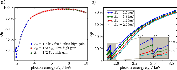
Figure 4: The quantum efficiency $\mathit{QE}$ of the detector, measured over the full energy range of the beamline with recommended settings (a) and for different threshold levels at the low end of the energy range (b). The green triangular symbols in (a) denote measurements using the high-gain mode, while all other data was measured using the ultra-high gain mode. The shaded areas around the data points indicate the relative uncertainty of the values (3 % in ultra-high gain mode, 1 % in high gain mode). The inset in (b) displays a close-up around the silicon K-edge. The ring current of the storage ring was reduced to 22 µA (6 µA) for photon energies above (below) $3.5\ \mathrm{keV}$, respectively.

The measured quantum efficiency with the associated uncertainty (shaded areas) is displayed in Figure 4. It depends not only on the photon energy $E_{\textrm{\small\scriptsize ph}}$, but also on the threshold level $E_{\textrm{\scriptsize thresh}}$ of the detector. Above $E_{\textrm{\small\scriptsize ph}}=3.4~{}\mathrm{keV}$, the threshold level was set to the preferred value $E_{\textrm{\scriptsize thresh}}=\frac{1}{2}E_{\textrm{\small ph}}$, which is shown in Figure 4a by the red square symbols for the ultra-high gain mode and by the green triangles for the high-gain mode. The high-gain mode is limited to threshold settings $E_{\textrm{\scriptsize thresh}}$ above $3.75~{}\mathrm{keV}$, or equivalently $E_{\textrm{\small\scriptsize ph}}$ to above $7.5~{}\mathrm{keV}$. Below $E_{\textrm{\small\scriptsize ph}}=3.4~{}\mathrm{keV}$, the threshold in ultra-high gain mode was fixed to $E_{\textrm{\scriptsize thresh}}=1.7\ \mathrm{keV}$ (blue circles in Figure 4a). In addition, the $\mathit{QE}$ was measured in this range for larger settings of $E_{\textrm{\scriptsize thresh}}$ up to $2.0~{}\mathrm{keV}$ (Figure 4b).

The $\mathit{QE}$ exceeds $80\ \%$ over the range from $3.4~{}\mathrm{keV}$ to $10~{}\mathrm{keV}$, with a maximum of $96\ \%$ at $8\ \mathrm{keV}$. Below $3~{}\mathrm{keV}$, the quantum efficiency is reduced due to the absorption of photons in the non-sensitive surface layers of the sensor, which are always present in semiconductor detectors Krumrey and Tegeler (1992). Just above the Si K-edge, the $\mathit{QE}$ drops to about $5\ \%$, however, measurements are feasible down to $1.75~{}\mathrm{keV}$. The measured $\mathit{QE}$, in particular at low energy, is in full agreement with the previously reported $\mathit{QE}$ of the single module test setup at the corresponding threshold setting Donath et al. (2013). The two different gain settings result in an difference less than $1\ \%$, which is within the uncertainty of the measurement. The threshold level settings have a noticeable influence, as displayed in Figure 4b. The highest $\mathit{QE}$ is achieved by the lowest possible threshold setting $E_{\textrm{\scriptsize thresh}}=1.7~{}\mathrm{keV}$, as expected Kraft et al. (2009a), and is therefore chosen as the recommended setting for all subsequent measurements.

It should be noted that the fill pattern of the electrons in the storage ring also has an influence on the registered count rate as described by Trueb et al. (2012). During our measurements, the circulation period was 800 ns, the electrons were divided in 350 bunches with a separation time of 2 ns and a dark gap of 100 ns. Since the detector dead-time in ultra-high gain mode of 4 µs corresponds to more than four cycles, the detector is completely insensitive to the fill pattern substructure. The fill pattern during our measurements is comparable to the data obtained at the Swiss Light Source and at the Australian Synchrotron as reported by Trueb et al., therefore, a similar systematic loss in the registered count rate should occur.

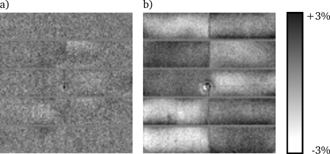
Figure 5: The homogeneity of the detector at a photon energy of (a) $10~{}\mathrm{keV}$ and (b) $5~{}\mathrm{keV}$ in ultra-high gain mode and with $E_{\textrm{\scriptsize thresh}}=\frac{1}{2}\,E_{\textrm{\small\scriptsize ph}}$. The raw data was preprocessed by binning $10\times 10$ pixels into one in order to overcome the quantum noise in comparison to the inhomogeneous detector response. The ring in the centre is an artefact which comes from the positioning of the beamstop to the centre of the scattering pattern.

In order to investigate possible variations in sensitivity over the detector area for fixed settings of energy, gain mode and threshold, a different approach was applied. SAXS images in the range from $4~{}\mathrm{keV}$ to $10~{}\mathrm{keV}$ were recorded using a sample of glassy carbon. The scattering pattern of glassy carbon exhibits a flat plateau in the range of the momentum transfer $q$ from $0.1\ \mathrm{nm^{-1}}$ to $1\ \mathrm{nm^{-1}}$ Zhang et al. (2010). Therefore, we achieve a nearly homogeneous illumination of the detector, which varies only in radial direction from the scattering centre. By dividing the whole image by the azimuthally averaged scattering curve pixel by pixel, we obtain an image with the relative deviation of each pixel value from the mean. Figure 5 displays the intensity deviation after averaging patches of $10\times 10$ pixels in order to reduce the shot noise. At $10~{}\mathrm{keV}$, the intensity difference amounts to $0.5\ \%$ across the whole detector, while at $5~{}\mathrm{keV}$, the intensity varies by $2.5\ \%$, although the manufacturer-supplied flat field correction was enabled. This discrepancy can be explained by the absorption of radiation in the upper insensitive layer of the detector. At high energies, this layer is nearly transparent, while at lower energies, the absorption and therefore the variation increase. This may result in a limited accuracy of the extrapolation of calibration values for trimming, which is based on flat field reference measurements at higher photon energies. The inhomogeneity can possibly be reduced by applying better flat field corrections in the low photon energy range from these images.

V Geometric characterization

A possible geometric distortion introduced by the detector must be known to determine uncertainty bounds for metrological nanodimensional measurements such as suggested, for example, in Krumrey et al. (2011); Wernecke, Scholze, and Krumrey (2012). A sequence of measurements was conducted in order to determine the pixel pitch, the displacement of the modules from their nominal position and the misalignment with respect to one another. This was achieved by measurement sequences, where the small-angle scattering of a selected sample was used to generate static test patterns, and the detector was moved to different positions for each image of the sequence.

The first sequence of measurements was conducted in SAXS geometry at $E_{\textrm{\small\scriptsize ph}}=8~{}\mathrm{keV}$ using the standard sample silver behenate, which displays an intense ring at $q=1.076\ \mathrm{nm^{-1}}$ Blanton et al. (1995). The detector was positioned at a distance of $d=2754\ \mathrm{mm}$ to the sample, and $240$ images were recorded. Between the exposures, the detector was vertically shifted in a stepwise fashion by moving both vertical translation axes $z_{1}$ and $z_{2}$ in parallel. The total distance by which the detector was moved amounts to $7\ \mathrm{mm}$. The traceability of the $z_{1}$ and $z_{2}$ movement was established by the Heidenhain linear encoders.

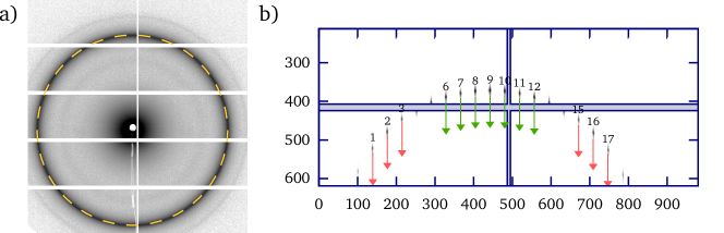
Figure 6: Test patterns for geometric measurements (a) SAXS image of silver behenate at 8 keV together with fit circle in dashed yellow. (b) GISAXS pattern (similar to Fig. 7) to determine the module alignment. Image series were recorded for vertical and horizontal displacement of the detector, here shown exemplary for a vertical movement along a module gap (grey shaded area). The numbered maxima indicate the peaks that were tracked to determine the detector movement (arrows show the nominal path along which 20 images were recorded). One group of peaks (6-12; green arrows) crosses the module borders, the other group (1-3 and 15-17; red arrows) stays on a module and is used for reference. The same procedure is applied to the other module gaps on the detector.

Next, a circle was fitted to every recorded image by maximizing the average intensity along the ring, which was represented by a Gaussian line with a width of $\sigma=1.06\ \mathrm{px}$. An example image together with the fitted circle (dashed line) is shown in Figure 6a. The best fit centre positions of these circles were then linearly fitted to the corresponding vertical detector displacement values $z_{1}$ and $z_{2}$. The residuals for this fit did not exceed one tenth of the pixel pitch for any circle position. From this linear fit, the pixel pitch $p=(172.1\pm 0.2)$ µm can be concluded. The uncertainty estimate of this value is derived from the comparison of both vertical shift axes and two independent measurements. The pure statistical error from the linear fit is smaller by an order of magnitude.

For the second sequence of measurements, the GISAXS pattern of a reflection grating with parallel alignment of grating lines and incident beam was used (see next section and Wernecke, Scholze, and Krumrey (2012)). This setup produces a series of equidistantly spaced sharp peaks ordered on an extended semicircle, which was used to characterize the placement of the individual detector modules with respect to each other. Figure 6b displays the positions of the peaks on the detector for one contiguous series of images. The detector was moved vertically upwards in 20 steps and an image was taken at every position. The peak positions were extracted from the images with subpixel resolution by computing the intensity-weighted centre of mass for every peak. The peaks can be divided into three categories. The peaks in the first category (labelled 1–3 and 15–17 in Figure 6b) stay on a single module. These were used as a reference trace. The peaks 6–10 and 11–12 cross the horizontal module borders between the upper and lower modules to the left and right, respectively. The remaining peaks (unlabelled) are neither confined to a single module nor do they cross the module borders completely to reach the next module. Similar datasets were recorded for all module borders in the horizontal and vertical direction.

The relative displacement of the modules from the nominal position results in a discontinuity of the trace for the border-crossing peaks. However, on the subpixel scale it has to be considered that the movement of the detector is slightly irregular due to deviations of the mechanical positioning. By comparing the border-crossing traces with the reference peak traces, the discontinuity can be detected regardless of an irregularly shaped path. The analysis was performed by least-squares fitting of the reference trace to the border-crossing traces at both sides of the gap. The maximum deviation from the nominal position amounts to 60 µm over the whole detector, which is less than 1 pixel.

In principle, the same method could be used to determine the in-plane angular misalignment between two neighbouring modules. The angular deviation was found to be below 0.1°, but this is already beyond the limit of this method due to the limited resolution of the peak- centre finding of $\approx 20$ µm. An out-of-plane angular misalignment leads only to smaller pixel length in the direction perpendicular to the axis of rotation. A deviation was measured for the same detector with great sensitivity by Bragg diffraction at the surface of the detector Gollwitzer and Krumrey (2013), with a result of a deviation of at most 0.4°. However, we cannot distinguish whether the deviation originates from a possible miscut of the silicon wafers or from a mechanical misalignment of the modules. Since the cosine of this angle deviates by less than 25 ppm from unity, this has no effect on the scattering images.

VI Application example: GISAXS at low photon energies

One of the advantages of a lower X-ray photon energy in SAXS and GISAXS experiments is the increased resolution (at a given experimental geometry). Consequently, the scattering pattern of larger structures can be resolved and the precision in determining smaller scattering lengths increases due to a larger separation distance of scattering features. In X-ray scattering, the reciprocal space is mapped. In SAXS and GISAXS, this is manifested in an intensity pattern of the diffusely scattered beam that is recorded by the 2-dimensional detector. For GISAXS, the relevant momentum transfer coordinates are

$$q_{y}=k_{0}\;\left(\sin\theta_{f}\cos\alpha_{f}\right);\ q_{z}=k_{0}\;\left(\sin\alpha_{f}+\sin\alpha_{i}\right)$$ (1)

with the wavenumber $k_{0}=2\pi/\lambda$, the incident angle $\alpha_{i}$, and the vertical and horizontal scattering angles $\alpha_{f}$ and $\theta_{f}$, respectively. From (1) it becomes clear that a reduction of photon energy (i.e., increase of wavelength $\lambda$) at a given geometry results in a decrease of the probed $q$-range and an increase of the $q$-resolution of the detector image. This has high practical relevance in nanometrological GISAXS measurements of sub-µm and nm-spaced gratings Wernecke, Scholze, and Krumrey (2012); Hofmann, Dobisz, and Ocko (2009). The aim of such measurements is to establish a traceable determination of the grating period, line width, and other structural parameters. This may serve as a basis to evaluate the general accuracy of the GISAXS method itself and gives more meaning to any length determined with GISAXS by an associated uncertainty. Here, the benefit of an increased $q$-resolution is a reduction of the grating parameter uncertainty.

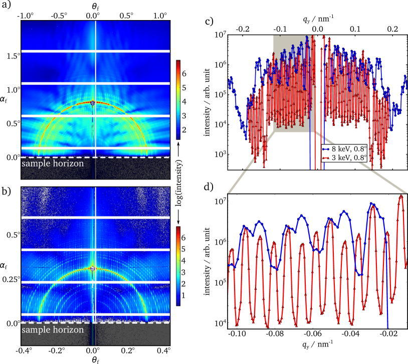
Figure 7: GISAXS scattering pattern of a line grating with a period length of 833 nm in parallel orientation of grating lines and incident beam, recorded at (a) $8~{}\mathrm{keV}$ and (b) $3~{}\mathrm{keV}$ (incident angle 0.8° in both cases). (c) Intensity profiles along the semicircles of the GISAXS patterns. (d) Close-up of the $q_{y}$-range from $-0.11~{}\textrm{\small nm}^{-1}$ to $-0.01~{}\textrm{\small nm}^{-1}$.

Figure 7a shows a typical GISAXS pattern for parallel orientation between the incident X-ray beam and the grating lines with an incident angle of $\alpha_{i}$ = 0.8°. The most prominent feature is a semicircle with evenly spaced intensity maxima. The modulation of these maxima is governed by the characteristic scattering lengths that are present in the sample Mikulík et al. (2001); Yan and Gibaud (2007). Hence, by analysing the frequencies of the intensity profile along the semicircle, the period length and line width of the grating can be directly determined from the scattering pattern Wernecke, Scholze, and Krumrey (2012). The GISAXS images recorded at 8 keV, Figure 7a, and at 3 keV, Figure 7b, already show the enlarged separation distance of maxima at the lower energy. Figure 7c shows the intensity profiles along the semicircle as a function of $q_{y}$ for both energies. The profiles and the close-up of the region left of the beamstop (at around $q_{y}$ = 0 nm^-1) in Figure 7d show the significantly pronounced oscillations and the increased number of data points per peak at 3 keV. This allows a more precise identification of the oscillation frequencies of the signal, which in turn results in lower uncertainties of the structural grating parameters determined.

VII Conclusion

A vacuum-compatible version of the PILATUS 1M detector has been installed at the PTB four-crystal monochromator beamline and enables scattering measurements down to a photon energy of $1.75\ \mathrm{keV}$, which is below the K-absorption edge of silicon and other light elements also relevant for biological and organic systems. The quantum efficiency has been determined in the entire range provided by the FCM beamline with a relative uncertainty of $3\ \%$ in ultra-high gain mode and $1\%$ in high gain mode. The quantum efficiency is excellent ($>80\ \%$) above $3.4\ \mathrm{keV}$ and provides a sufficient signal for X-ray scattering measurements at lower photon energies down to $1.75\ \mathrm{keV}$. The geometric distortions of the detector due to deviations in module placement stay below 1 pixel over the whole detector. The first scattering experiments show the extended capabilities of the detector due to the increased resolution in $q$ at low energies. SAXS and GISAXS measurements on biological samples and nanostructured polymer thin films are currently being analysed and will be published soon. Further insight into the internal structure is expected from the element-selective tuning of the scattering contrast of the contained light elements.