H I FREE-BOUND EMISSION OF PLANETARY NEBULAE WITH LARGE ABUNDANCE DISCREPANCIES: TWO-COMPONENT MODELS VERSUS $\kappa$-DISTRIBUTED ELECTRONS

Abstract

The “abundance discrepancy” problem in the study of planetary nebulae (PNe), viz., the problem concerning systematically higher heavy-element abundances derived from optical recombination lines relative to those from collisionally excited lines, has been under discussion for decades, but no consensus on its solution has yet been reached. In this paper we investigate the hydrogen free-bound emission near the Balmer jump region of four PNe that are among those with the largest abundance discrepancies, aiming to examine two recently proposed solutions to this problem: two-component models and $\kappa$ electron energy distributions. We find that the Balmer jump intensities and the spectrum slopes cannot be simultaneously matched by the theoretical calculations based upon single Maxwell-Boltzmann electron-energy distributions, whereas the fitting can be equally improved by introducing $\kappa$ electron energy distributions or an additional Maxwell-Boltzmann component. We show that although H I free-bound emission alone cannot distinguish the two scenarios, it can provide important constraints on the electron energy distributions, especially for cold and low-$\kappa$ plasmas.

1 INTRODUCTION

The determination of element abundances in planetary nebulae (PNe) is essential for understanding the stellar nucleosynthesis processes and the chemical enrichment in the interstellar medium. However, a number of studies of PNe have consistently established an intriguing puzzle that heavy-element abundances determined from optical recombination lines (ORLs) are systematically higher than those derived from collisionally excited lines (CELs). The abundance discrepancy is commonly quantified by the ratio between the O²⁺ abundances obtained from ORLs and CELs, called abundance discrepancy factor (ADF). The CEL abundance determination is subject to an accurate determination of the electron temperature. A relevant problem is that the electron temperatures obtained from the H I Balmer jump are generally lower than those obtained from [O III] CELs (to be referred to as $T_{\rm e}$(BJ) and $T_{\rm e}$([O III]), respectively, hereafter). The ADFs have been found to be positively correlated with the temperature differences (Liu et al., 2001). Several explanations for the abundance and temperature discrepancies have been proposed, but no consensus has emerged (see, Peimbert, 1967; Liu & Danziger, 1993; Stasińska, 2004; Liu, 2006; Peimbert & Peimbert, 2006, and the references therein for further details on the two problems), among which we will focus on two here: two-component models and $\kappa$-distributed electrons.

The two-component models assume that there exist spatially unresolved knots within diffuse nebulae (Liu et al., 2000). These knots are extremely metal-rich and partially or fully ionized. Because of high cooling rates, they have relatively low temperatures, which therefore greatly favor the emission of ORLs and suppress that of CELs. It follows that in the scenario of two-component models, ORLs and CELs inform us about the abundances and electron temperatures in different nebular components. Detailed three-dimensional photoionization models of NGC 6153, a PN exhibiting a large ADF, show that the two-component models incorporating a small amount of metal-rich inclusions can successfully reproduce all the observations (Yuan et al., 2011). The chemical pattern can exclude the ejection of stellar nucleosynthesis products as the origin of these knots. Liu (2006) suggested that they might be produced by evaporating planetesimals. The hypothesis of solid body destruction was theoretically investigated by Henney & Stasińska (2010), who concluded that under certain conditions the sublimation of volatile bodies possibly produces enough metal-rich gas to explain the ORL/CEL abundance discrepancies. The main criticism of this model is that there is no direct observational evidence for the existance of such knots.

Previous calculations of element abundances and electron temperatures in PNe have been based upon a widely accepted assumption that free electrons have Maxwell-Boltzmann (M-B) energy distributions (Spitzer, 1948). Recently, Nicholls et al. (2012, 2013) presented that the presence of non-thermal electrons can potentially account for the abundance and temperature discrepancy problems. In this scenario, the free electrons have non-equilibrium energy distributions whose departure from M-B distributions can be parameterized by a $\kappa$ index. Such a $\kappa$ distribution involves a low-temperature M-B core and a power-law high energy tail, and has been applied to fit the energy distributions of energetic particles in solar system plasmas (e.g. Livadiotis & McComas, 2011). Since the low- and high-energy electrons are preferential for recombination and collision processes, respectively, ORLs would indicate a lower electron temperature than CELs if using an M-B distribution to interpret the spectrum with a $\kappa$ distribution. Leubner (2002) and Livadiotis & McComas (2009) show that the phenomenologically introduced $\kappa$ distributions in the studies of solar system plasmas can arise naturally from Tsallis’ nonextensive statistical mechanics. In collisionless plasmas, it takes a long time for high-energy electrons to relax to their equilibrium distribution, which thus can reach a non-equilibrium stationary state if they can be continuously pumped. The physical mechanisms producing non-thermal electrons in PNe, however, have never been thoroughly investigated, although Nicholls et al. (2013) sketched a few possibilities.

Apparently, measuring the electron energy distribution from observations is important to examine the two propositions. For this purpose, Storey & Sochi (2013) studied C II dielectronic recombination lines in a few PNe, but the uncertainties are too large to draw any definite conclusion. To further investigate the two scenarios, in this paper we study the hydrogen free-bound continua of four PNe with very large ADFs ($>6$). In Section 2, we present the methodology and discuss the possibility of using hydrogen free-bound continua as a probe of the electron energy distribution. In Section 3, we fit the observed spectra with theoretical calculations of two-component models and $\kappa$-distributed electrons, and discuss the implications of these results. Section 4 is a summary of our conclusions.

2 METHODOLOGY

The H I free-bound spectrum is emitted when a free electron is captured by a proton, and thus can potentially sample the energy distribution of recombining electrons. Below we present the calculations of H I free-bound spectra near the Balmer jump region in M-B and $\kappa$ electron energy distributions, followed by a brief description of the PN sample and the spectral fitting procedure.

2.1 H I free-bound emission from M-B electron distributions

The H I continuous spectrum is calculated using the same method as described in Zhang et al. (2004). Assuming that free electrons have an M-B energy distribution, viz.,

$$\frac{n(E)}{N}dE=2\sqrt{\frac{E}{\pi}}\left(\frac{1}{k_{B}T_{U}}\right)^{3/2}{\rm e}^{-E/k_{B}T_{U}}dE,$$ (1)

the emission coefficient of H I free-bound continuous emission is given by

$$j_{\nu}^{\rm M-B}=\frac{1}{4\pi}N_{\rm p}N_{\rm e}\frac{\pi h^{4}\nu^{3}}{c^{2}}\left(\frac{2}{\pi m_{\rm e}k_{B}T_{U}}\right)^{3/2}\sum_{n=n_{1}}^{\infty}\sum_{l=0}^{n-1}n^{2}a_{nl}(\nu){\rm e}^{h(\nu_{nl}-\nu)/k_{B}T_{U}},$$ (2)

where $k_{B}$ and $h$ are the Boltzmann and the Planck constants, respectively, $c$ is the speed of light, $m_{\rm e}$ is the electron mass, $N_{\rm p}$ and $N_{\rm e}$ are proton and electron densities respectively, $h\nu_{nl}$ is the ionization potential of the ($n$,$l$) state, $n_{1}$ is the lowest state that can contribute to the free-bound emission at the given frequency $\nu$ ($n_{1}=2$ and 3 for the Balmer and Paschen recombination continua, respectively), and $a_{nl}(\nu)$ is the photoionization cross-section for the state, which is computed using the method described by Storey & Hummer (1991). $T_{U}$ is the kinetic temperature reflecting the internal energy of free electrons, which under the M-B distribution is commonly referred to as electron temperature, $T_{\rm e}$. Free-free emission and two-photon decay are also taken into account (see Zhang et al., 2004, for the details). The spectrum then is normalized to the integrated intensity of the H11 Balmer line at 3770 Å, whose emission coefficient is given by

$$j_{{\rm H}11}^{\rm M-B}=\frac{1}{4\pi}N_{\rm p}N_{\rm e}\alpha^{\rm eff}_{{\rm H}11}h\nu_{{\rm H}11},$$ (3)

where $\alpha^{\rm eff}_{{\rm H}11}$ is the effective recombination coefficient of the H11 line derived by Hummer & Storey (1987) based upon M-B electron distributions. Hereafter, we use $I_{\lambda}$, in units of Å^-1, to denote the normalized continuum intensity.

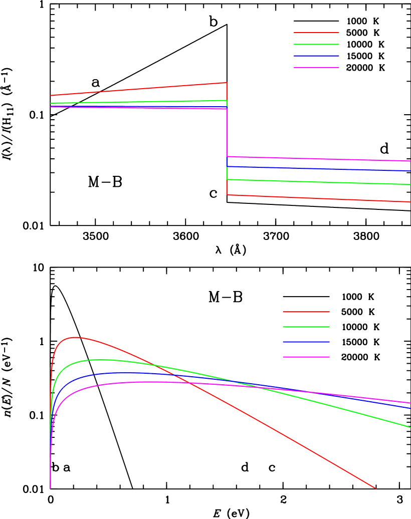
Figure 1: Theoretical hydrogen free-bound continua near the Balmer jump region (upper panel) for single M-B electron distributions (lower panel) at different temperatures. The spectral shapes in the upper panel can be characterized by the labeled ‘abcd’, which trace the recombining electrons with kinetic energies marked in the lower panel.

In Figure 1 we show the calculated H I free-bound spectra near the Balmer jump region at different $T_{U}$ values along with the corresponding electron energy distributions. It is apparent from this figure that the shapes of theoretical spectra strongly depend on the electron energy distributions. We choose four positions, as labeled in Figure 1 (‘abcd’, where $\lambda_{a}=3500$ Å, $\lambda_{b}=3650^{-}$ Å, $\lambda_{c}=3650^{+}$ Å, and $\lambda_{d}=3900$ Å), to characterize the spectra, and thus the spectral shapes can be quantitatively described with the slopes of the Balmer continuum $S_{B}=(I_{b}-I_{a})/(\lambda_{a}-\lambda_{b})$ and the Balmer jump $J_{B}=I_{b}-I_{c}$. The a–b and c–d spectra are respectively produced by free electrons recombining to $n=2$ and 3 states, whose kinetic energies satisfy the relation $E_{b}(0\,{\rm eV})<E_{a}(0.14\,{\rm eV})<E_{d}(1.67\,{\rm eV})<E_{c}(1.89\,{\rm eV})$. An inspection of Figure 1 reveals that with increasing kinetic temperatures, $S_{B}$ and $J_{B}$ decrease while $I_{c}$ and $I_{d}$ increase. This is clearly due to the increasing number of high-energy electrons with respect to low-energy electrons. At high kinetic temperatures ($T_{U}>10000$ K), the $S_{B}$ and $J_{B}$ values become significantly less sensitive to $T_{U}$, attributing to the incapability of H I continua near the Balmer jump region to trace very energetic electrons. Consequently, the examination of Figure 1 indicates that H I free-bound continua can provide a potential probe of electron energy distributions in cold plasma.

2.2 H I free-bound emission from $\kappa$ electron distributions

The electron energy distributions in the vicinity of the Sun and a few planets have been found to have an M-B core and an enhanced high-energy tail, which can be well described by a $\kappa$ distribution (i.e. Livadiotis & McComas, 2009; Livadiotis et al., 2011) defined by

$$\frac{n(E)}{N}dE=2\sqrt{\frac{E}{\pi}}\left(\frac{1}{k_{B}T_{U}}\right)^{3/2}\frac{\Gamma(\kappa+1)}{(\kappa-3/2)^{3/2}\Gamma(\kappa-1/2)}\left[1+\frac{h(\nu_{nl}-\nu)}{(\kappa-3/2)k_{B}T_{U}}\right]^{-\kappa-1},$$ (4)

where $\Gamma$ is the gamma function and $\kappa$ is a parameter of $>1.5$ describing the degree of departure from the M-B distribution. This inspired Nicholls et al. (2012) to suggest that the $\kappa$ distribution also applies for the plasmas in PNe. As illustrated in Nicholls et al. (2012), at a given $T_{U}$, decreasing $\kappa$ values would cause a shift of the number of intermediate-energy electrons towards those of higher and lower energies. As a result, the low-energy region manifests its profile as an M-B distribution with an equilibrium temperature

$$T_{\rm core}=\left(1-\frac{3}{2\kappa}\right)T_{U}.$$ (5)

In the case of the $\kappa$ electron energy distribution, the emission coefficient of H I free-bound continuous emission can be written as

$$\begin{split}j_{\nu}^{\kappa}=&\frac{1}{4\pi}N_{\rm p}N_{\rm e}\frac{\pi h^{4}\nu^{3}}{c^{2}}\left(\frac{2}{\pi m_{\rm e}k_{B}T_{U}}\right)^{3/2}\frac{\Gamma(\kappa+1)}{(\kappa-3/2)^{3/2}\Gamma(\kappa-1/2)}\\ &\times\sum_{n=n_{1}}^{\infty}\sum_{l=0}^{n-1}n^{2}a_{nl}(\nu)\left[1+\frac{h(\nu_{nl}-\nu)}{(\kappa-3/2)k_{B}T_{U}}\right]^{-\kappa-1}.\end{split}$$ (6)

In the limit $\kappa\rightarrow\infty$, the $\kappa$ distribution tends to the M-B, and Equations (4) and (6) go over to Equations (1) and (2), respectively.

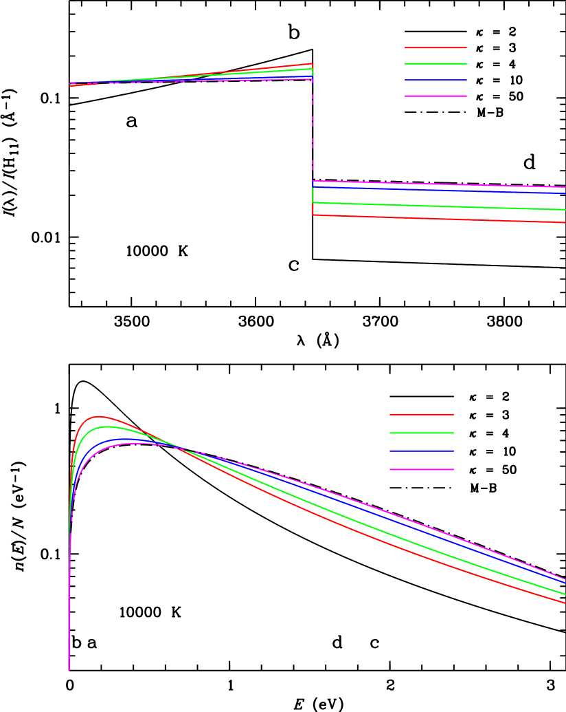
Figure 2: Theoretical hydrogen free-bound continua near the Balmer jump region (upper panel) for $\kappa$ and M-B electron distributions (lower panel) at 10000 K but different $\kappa$ values. Other details are the same as in Figure 1.

We investigated the behavior of H I free-bound spectra under $\kappa$ electron distributions. Figure 2 displays the calculated spectra at a given temperature $T_{U}=10000$ K but different $\kappa$ values, as well as the corresponding electron energy distributions. In order to obtain the normalized spectra, the recombination coefficient of the H11 line has been corrected according to Equation (17) in Nicholls et al. (2013), so that the emission coefficient is given by

$$j_{{\rm H}11}^{\kappa}=\frac{(1-3/2\kappa)\Gamma(\kappa+1)}{(\kappa-3/2)^{3/2}\Gamma(\kappa-1/2)}j_{{\rm H}11}^{\rm M-B}.$$ (7)

As shown in Figure 2, decreasing $\kappa$ values cause the peak of the electron distribution to move to lower energies (see the lower panel), resulting in increasing $J_{B}$ and $S_{B}$ and decreasing $I_{c}$ and $I_{d}$ (see the upper panel). The theoretical spectrum at a high $\kappa$ value is almost identical to that calculated based upon an M-B electron distribution of the same temperature. Therefore, in principle, one can determine the $\kappa$ value by comparing the theoretical and observed H I free-bound continua. This method is particularly suitable when the $\kappa$ value is low and thus the distribution of low-energy electrons is sensitive to its alteration. Because H I free-bound continua are insensitive to the $\kappa$ value when $\kappa$ is large, we choose a few extreme PNe with large ADFs for this study, which are supposed to have extremely low $\kappa$ values if the abundance discrepancies are caused by the $\kappa$ electron distribution.

In order to address the question whether the H I free-bound spectrum allows one to distinguish between $\kappa$ and M-B electron distributions, in Figure 3 we compared the spectra calculated based upon a $\kappa$ distribution at $T_{U}$ and an M-B distribution at $T_{\rm core}$, where $T_{U}$ and $T_{\rm core}$ satisfy the relation given by Equation (5). As shown in this figure, the Balmer continua (a–b) of the 10000 K $\kappa$ distribution and the 2500 K M-B distribution are nearly parallel, viz., the $S_{B}$ values are equal, which can be attributed to the fact that the profile of the cold M-B electron distribution closely resembles that of the low-energy region of the $\kappa$ one. However, the 2500 K M-B distribution predicts a larger $J_{B}$ value, which is conceivable since its peak $n(E)/E$ value is larger (see the lower panel of Figure 3). Since the temperature-only-dependent M-B distributions indicate a one-to-one correspondence between $S_{B}$ and $J_{B}$ (Figure 1), it follows that the H I free-bound continua provide a diagnostic to separate the two kinds of electron distributions, and $S_{B}$ and $J_{B}$ can be used to evaluate the $\kappa$ value. Another implication of our calculations is that using an M-B electron distribution one is unable to simultaneously match the $S_{B}$ and $J_{B}$ values of the H I free-bound continua arising from a $\kappa$ electron distribution, in that $J_{B}$ will imply a higher M-B temperature than $S_{B}$.

2.3 The sample and spectral fitting

Our sample includes four PNe, Hf 2-2, NGC 6153, M 1-42, and M 2-36, which are among the PNe exhibiting the largest temperature and abundance discrepancies. The high signal-to-noise spectra are taken from Liu et al. (2000, 2001, 2006), whose primary purpose was to measure the intensities of weak ORLs from heavy-element ions. Careful treatments have been devoted to flux calibrations and dereddening corrections (see Liu et al., 2000, 2001, 2006, for the details). Table 1 gives the ADFs, $T_{\rm e}$(BJ), and $T_{\rm e}$([O III]) deduced through the empirical analysis. Their ADFs range from 6.9 to 70, much larger than the average value of Galactic PNe ($\sim 2$). The $T_{\rm e}$([O III]) values are found to be higher than $T_{\rm e}$(BJ) by a factor of 1.4–9.4.

In order to fit the observed H I free-bound continua, we consider three possibilities for electron energy distributions: single M-B distributions, bi-M-B distributions, and $\kappa$ distributions. The former has a single fitting parameter (i.e. the electron temperature), while the later two have two parameters (see the next section). The reduced $\chi^{2}$ values were calculated in a parameter space for each object to evaluate the goodness of fit, which is defined by

$$\chi^{2}=\frac{1}{\eta}\sum\frac{(I_{\lambda,\rm obs}-I_{\lambda,\rm the})^{2}}{\sigma_{\lambda}^{2}},$$ (8)

where $I_{\lambda,\rm obs}$ and $I_{\lambda,\rm the}$ are the observational and theoretical continuum intensities in the line-free regions of the spectrum ranging from 3200–4200 Å, $\sigma_{\lambda}$ is the measurement error of $I_{\lambda,\rm obs}$ caused by noises, and $\eta$ is the number of degrees of freedom. The optimal fitting for each object is then achieved with the temperature and/or other fitting parameters that yield the minimum $\chi^{2}$ value.

In addition to H I recombination continua, the observed spectra contain a contamination from the direct or scattered light from the central star. Consequently, the theoretical continuum intensity is given by

$$I_{\lambda,\rm the}=I_{\lambda,\rm star}+I_{\lambda,\rm H},$$ (9)

where the theoretical H I recombination intensity $I_{\lambda,\rm H}$ is a sum of contributions from free-bound, free-free, and two-photon emission, among which the free-bound transition dominates the spectrum near the Balmer jump, and the free-free emission is negligible. In order to minimize the number of fitting parameters, we assume that the spectral energy distribution of the contaminating stellar continuum follows a power law,

$$I_{\lambda,\rm star}=(I_{b,\rm obs}-I_{b,\rm H})(\lambda_{b}/\lambda)^{-\beta},$$ (10)

where $I_{b,\rm obs}$ and $I_{b,\rm H}$ are the observational continuum intensity and theoretical H I recombination intensity at $\lambda_{b}=3650^{-}$ Å, respectively. $I_{\lambda,\rm star}$ is initially assumed to follow a Rayleigh-Jeans approximation to a blackbody, viz., $\beta=4$. However, the actual situation might be more complex because of the wavelength and spatial dependence of scattered light. Moreover, there is some uncertainties in the emission coefficient of the two-photon process that can affect the calculations of continuum intensity (see Zhang et al., 2004). Therefore, $\beta$ is slightly adjustable, and we adopt $\beta$ to be an integer between 2 and 5 yielding the best fit.

3 RESULTS and DISCUSSION

The fitting results are shown in Table 1. We find that for all the PNe the observed continua cannot be successfully fitted with the theoretical spectra calculated by Equation 2 for single M-B electron energy distributions. In Figure 4 we plot the temperature dependences of $\chi^{2}$ in the one-parameter model. The distributions of filled circles in Figure 4 are less dense in the low-temperature side, attributing to the fact that the sensitivity of H I recombination spectra to temperature increases with decreasing $T_{\rm e}$. The minimum $\chi^{2}$ values in the range of $300\,{\rm K}<T_{\rm e}<25000\,{\rm K}$ are unacceptably large ($>4$). Specifically, $S_{B}$ and $J_{B}$ cannot be simultaneously matched by the one-parameter model. As indicated in Figure 5, the temperatures determined by $J_{B}$ are higher than those by $S_{B}$. This is a clear evidence that there is an excess of high-energy electrons with respect to the M-B distribution indicated by low-energy electrons (i.e. the fractional population of electrons at $E_{d}$ and $E_{c}$ is higher than that inferred from the electrons at $E_{a}$ and $E_{b}$; see Figure 1). Qualitatively saying, the excess of high-energy electrons can be caused by either bi-B-M (the two-component model) or $\kappa$ electron energy distributions. Below we investigate the two scenarios.

The two-component model assumes that nebular spectra arise from two gaseous components with different equilibrium temperatures, $T_{h}$ and $T_{c}$, representing electron temperatures of the hot diffuse nebulosities and the cold metal-rich knots, respectively (hereafter super- or subscript “$h$” and “$c$” refer to quantities of the hot and cold compoents, respectively). In this scenario, the theoretical H I recombination spectrum is a sum of contributions from the two components with individual M-B electron distributions, with the intensity of

$$I_{\lambda,\rm H}=\frac{f}{f+1}I_{\lambda,{\rm H}}^{c}+\frac{1}{f+1}I_{\lambda,{\rm H}}^{h},$$ (11)

where $f$ is the H11 line intensity ratio of the cold component over the hot component. Thus we have

$$f=\frac{N_{{\rm p},c}M_{{\rm e},c}\alpha^{\rm eff}_{{\rm H}11,c}}{N_{{\rm p},h}M_{{\rm e},h}\alpha^{\rm eff}_{{\rm H}11,h}},$$ (12)

where $M_{\rm e}$ is the total electron number of each component. A detailed photoionization model involving the two components has been successful in accounting for the spectrum of NGC 6153 (Yuan et al., 2011). Guided by the model of Yuan et al. (2011), we assume that $T_{h}/T_{c}\equiv 10$ and $N_{{\rm p},c}/N_{{\rm p},h}\equiv 5$ for all the PNe. Consequently, two parameters, $T_{h}$ and $M_{{\rm e},c}/M_{{\rm e},h}$, are employed for the two-component model fitting.

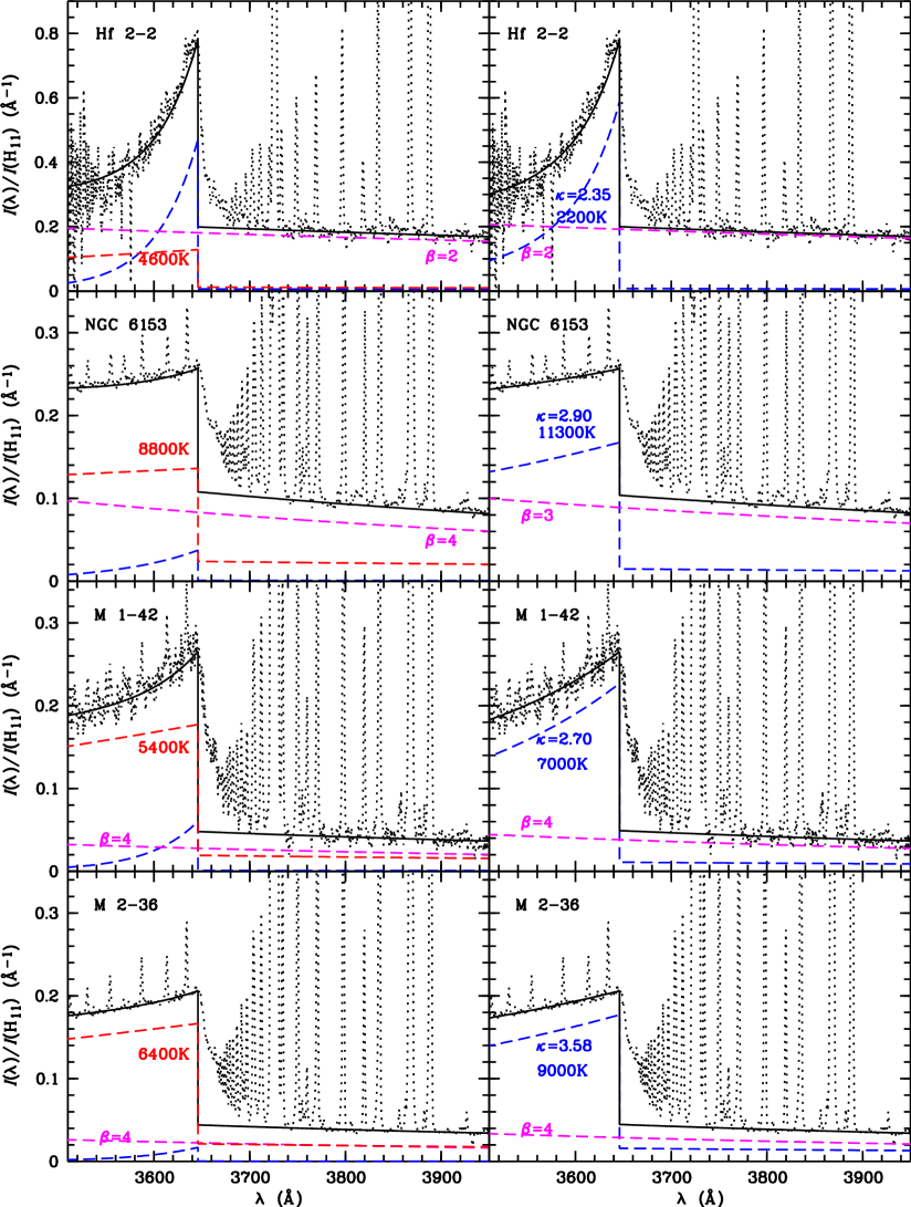
Figure 6: Fitting the hydrogen continua near the Balmer jump region using two-component models (left panel) and $\kappa$ electron distributions (right panel). In the left panel, the blue and red dashed curves denote the cold and hot nebular continua, respectively. Other details are the same as in Figure 5.

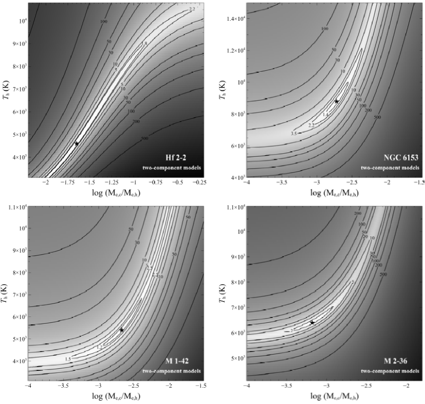
Figure 7: The $\chi^{2}$ contours of continuum fitting of the two-component models as a function of $M_{e,c}/M_{e,h}$ and $T_{h}$. The grey levels are proportional to the logarithm of $\chi^{2}$. The stars mark the best-fit values, as shown in the left panels of Figure 6.

Through introducing an additional component, the fitting is greatly improved (Table 1). The best fits are shown in Figure 6. Figure 7 shows the $\chi^{2}$ distributions in the parameter space that we search for. We find that this model is capable of producing $S_{B}$ and $J_{B}$ by including only small amount of cold components with $M_{{\rm e},c}/M_{{\rm e},h}$ ratios of $<0.03$. The contours of the $\chi^{2}$ values elongate along the increment direction of $T_{h}$ and $M_{{\rm e},c}/M_{{\rm e},h}$ (Figure 7), along which the fits are less sensitive to the choice of the fitting parameters. This simply reflects the fact that to account for the observations the increasing inclusion of cold component will result in higher $T_{h}$ values. Through reconciling $T_{h}$ and $T_{\rm e}$([O III]), the temperature discrepancy problem can be solved.

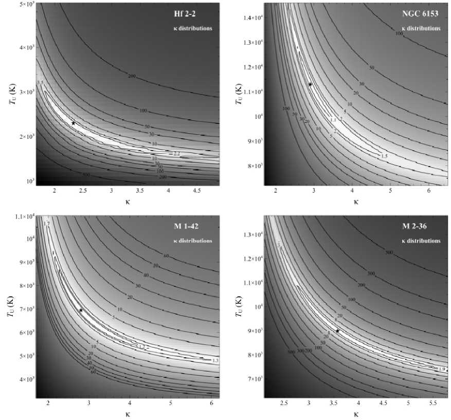
Figure 8: The $\chi^{2}$ contours of continuum fitting of the $\kappa$ electron energy distributions as a function of $\kappa$ and $T_{U}$. The grey levels are proportional to the logarithm of $\chi^{2}$. The stars mark the best-fit values, as shown in the right panels of Figure 6.

In the case of $\kappa$ electron distributions, $I_{\lambda,\rm H}$ is calculated based upon Equation (6), and $T_{U}$ and $\kappa$ are used as input parameters in the fitting procedure. Similar to the two-component model, the introduction of $\kappa$ electron distributions can significantly improve the fitting such that the minimum $\chi^{2}$ values can reach $<1.5$ (Table 1). The $\chi^{2}$ distributions in the $T_{U}$-$\kappa$ space are shown in Figure 8. A decreasing $\kappa$ value can lead to an increment of $T_{U}$ to accommodate the observed $S_{B}$ and $J_{B}$. The best fits, as shown in Figure 6, indicate very low $\kappa$ values for all the PNe, suggesting a large departure from the M-B distribution for these high-ADF PNe.

The elongation direction of the contours of $\chi^{2}$ (Figure 8) is a reflection of the fitting uncertainties, which suggests that $\kappa$ can be more accurately determined in the plasma more significantly departing from the M-B electron distribution. However, there is a long tail toward large $\kappa$ values. For NGC 6153 and M 1-42, a $\kappa$ value of $\sim 8$ can still achieve a reasonable match within the confidence level of $\chi^{2}<2.0$. Despite the large uncertainty, we can conclude that the $\kappa$ value for Hf 2-2 is extremely low. Such low $\kappa$ indexes have been found in inner heliosheath, blazar $\gamma$-rays, solar flares, interplanetary shocks, corotating interaction regions, and solar wind (Livadiotis et al., 2011). Various theories have been developed to explain the $\kappa$ distributions in solar system plasmas (Pierrard, 2010, and the references therein). The environments of PNe are very different. What physical mechanism is responsible for producing such a large population of non-thermal electrons in PNe remains a subject for speculation.

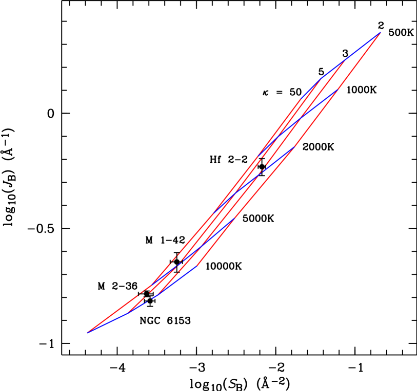
Figure 10: $J_{B}$ versus $S_{B}$ as functions of $\kappa$ values from 2–50 and kinetic temperatures from 500–10000 K. Note that the curve for $\kappa=50$ essentially coincides with that for single M-B electron distributions. The description of measured values given for Figure 9 applies.

We have shown that both the two-component models and $\kappa$ electron distributions can provide better agreement with the observations of H I continua than single M-B electron distributions. In the framework of a certain model, the H I continua behave differently for different parameter settings, and thus can provide a diagnostic to determine these parameters. In Figures 9 and 10, we plot the plasma diagnostics for the two-component models and $\kappa$ electron distributions, respectively. An inspection of the two figures suggests that with accurate subtraction of stellar light contamination it is possible to use $J_{B}$ and $S_{B}$ to derive $T_{U}$, $M_{{\rm e},c}/M_{{\rm e},h}$, and $\kappa$. The method is particularly useful for cold and/or low-$\kappa$ PNe. All the four PNe exhibit departure from the predictions of single M-B distributions (which coincide with those for $M_{{\rm e},c}/M_{{\rm e},h}=0.0002$ and $\kappa=50$ respectively in Figures 9 and 10), the most extreme one of which is Hf 2-2.

In this study, we do not take into account high order hydrogen recombination lines, which converge at the Balmer discontinuity (Figure 5) and are usually used to measure the electron density (e.g. Zhang et al., 2004). It is valuable to investigate their behavior under $\kappa$ electron distributions in the future.

The two-component models and $\kappa$-distributed electrons can improve the fit of nebular spectra near the Balmer jump region to a similar extent. Therefore, based on the H I free-bound continua alone, we cannot ascertain which scenario is more appropriate. However, the two-component models are perhaps more physically motivated. It suggests that PNe are spatially inhomogeneous in temperature, density, and chemical abundance. The cold knots embedded in diffuse nebulae are produced by the destruction of solid bodies, leading to a contamination of nebular spectra. Since the destruction of solid bodies is related to their spatial distributions and evolutionary stages of central stars, the two-component models can account for the observations that ADFs are larger in more evolved PNe and/or in the inner regions of a given PN. Furthermore, this model can provide plausible explanations for the observational facts that abundances derived from the temperature-insensitive infrared CELs are comparable with those from optical CELs, and the ORL abundances of high-ADF PNe are far beyond the predictions of stellar nucleosynthesis. The $\kappa$ distributions have been familiar to the solar physics community for decades. Such distributions have been proven to better match the observations of solar system plasmas than bi-M-B distributions. The $\kappa$ function was initially introduced as a mathematical description of energy distributions. As shown by Leubner (2002) and Livadiotis & McComas (2009), a $\kappa$ distribution is a consequence of Tsallis’s nonextensive statistical mechanics, yet its exact origin in solar system plasmas, and whether such an origin also works for photoionized gaseous nebulae, remains unclear.

4 CONCLUSIONS

In this paper, we investigate the H I free-bound continua of four PNe exhibiting extremely large ADFs. We find strong evidence that these spectra are not emitted from the plasma with single M-B electron energy distributions. Two possible explanations are examined: two-component models and $\kappa$-distributed electrons. Our results show that both can adequately account for the observations. We also present a method to determine the physical conditions of PNe with two components or $\kappa$-distributed electrons. Specifically, the H I Balmer jump $J_{B}$ and the slope of Balmer continuum $S_{B}$ can be used to derive temperature, filling factor of cold knots, and $\kappa$ index. The results presented in this paper provide new insights into the long-standing problem of abundance discrepancies in PNe.

Energy distributions of free electrons have a profound effect on abundance calculations of PNe. The recombination coefficients of ORLs and the collision strengths of CELs rely on the integral of the known energy dependence of the atomic cross section over the assumed distribution function. Unlike for solar system plasmas, whose energy distributions can been accurately detected through the direct interaction between the plasma particles and the detectors on-board satellites and space probes, it is rather hard to measure the electron energy distributions of distant PNe. H I free-bound spectra, which directly sample free electrons, provide a promising approach for such a purpose, and this paper can be regarded as a preliminary attempt. In future studies, we will further investigate this problem by obtaining high signal-to-noise spectra with wider wavelength coverage and utilizing O II and [O III] emission lines. This allows us to sample the free electrons with a wider energy coverage. For such an effort, very careful flux calibrations, reddening corrections, and subtractions of stellar light contamination are desirable.

Figure 3: Theoretical hydrogen free-bound continua near the Balmer jump region (upper panel) for $\kappa=2$ and M-B electron distributions at 10000 K as well as a ‘core’ M-B electron distribution at 2500 K (lower panel). In the lower panel, the areas under the three curves are all equal to 1, and the M-B core can fit the low-energy region of the $\kappa=2$ distribution by scaling a factor of $<1$. Other details are the same as in Figure 1.

Figure 4: $\chi^{2}$ versus $T_{\rm e}$ for the fitting based upon single M-B electron distributions. The filled circles represent an equal-interval scale of $T_{\rm e}$.

Figure 5: Fitting the Balmer jump ($J_{B}$; left panel) and the slope of Balmer continua ($S_{B}$; right panel) using single M-B electron distributions. The blue and magenta dashed curves denote the theoretical nebular continua and scattered stellar light, respectively. Note that no scattered stellar light is required to fit the $S_{B}$ value of M 1-42. The black solid and dotted curves are the synthetic and dereddened observed spectra, respectively. Note that $J_{B}$ and $S_{B}$ (especially for Hf 2-2) cannot be simultaneously fitted.

Figure 9: $J_{B}$ versus $S_{B}$ as functions of M_e,c/M_e,h values from 0.0002–0.01 and $T_{h}$ from 3000–14000 K in the two-component model. Note that the curve for M_e,c/M${}_{e,h}=0.0002$ essentially coincides with that for single M-B electron distributions. The measured values of the four PNe are also labeled. Errors bars indicate the measurement uncertainties. Note that because of the unsubtracted scattered stellar light, the filled circles represent the lower limits of $S_{B}$.

Table 1: Fitting parameters

Parameters	Hf 2-2	NGC 6153	M 1-42	M 2-36
ADFa	70	10	22	6.9
$T_{\rm e}$([O III])a (K)	8740	9110	9220	8380
$T_{\rm e}$(BJ)a (K)	930	6080	3560	5900
Single M-B electron energy distributions
$T_{\rm e}$ (K)	1100	6200	3800	5700
$\chi^{2}$	6.99	6.14	5.17	4.24
Two-component models
$T_{h}$ (K)	4600	8800	5400	6400
$M_{e,c}/M_{e,h}$ ($10^{-2}$)	2.24	0.20	0.22	0.06
$\chi^{2}$	1.02	1.12	1.08	1.27
$\kappa$ electron energy distributions
$T_{U}$ (K)	2200	11300	7000	9000
$\kappa$	2.35	2.90	2.70	3.58
$\chi^{2}$	1.03	0.99	1.08	1.45

^a From Liu et al. (2000, 2001, 2006).

References

- Henney & Stasińska (2010) Henney, W. J. & Stasińska, G. 2010, ApJ, 711, 881
- Hummer & Storey (1987) Hummer, D. G., & Storey, P. J. 1987, MNRAS, 224, 801
- Leubner (2002) Leubner, M. P. 2002, Ap&SS, 282, 573
- Liu (2006) Liu, X.-W. 2006, in IAU Symp. 234 Planetary Nebulae, eds. M. J. Barlow, & R. H. Méndez (Cambridge: Cambridge Univ. Press), 219
- Liu et al. (2006) Liu, X.-W., Barlow, M. J., Zhang, Y., Bastin, R. J., & Storey, P. J. 2006, MNRAS, 368, 1959
- Liu & Danziger (1993) Liu, X.-W., & Danziger, I. J. 1993, MNRAS, 263, 256
- Liu et al. (2001) Liu, X.-W., Luo, S.-G., Barlow, M. J., Danziger, I. J., & Storey, P. J. 2001, MNRAS, 327, 141
- Liu et al. (2000) Liu, X.-W., Storey, P. J., Barlow, M. J., et al. 2000, MNRAS, 312, 585
- Livadiotis & McComas (2009) Livadiotis, G., & McComas, D. J. 2009, J. Geophys. Res., 114, A11105
- Livadiotis & McComas (2011) Livadiotis, G., & McComas, D. J. 2011, ApJ, 741, 88
- Livadiotis et al. (2011) Livadiotis, G., McComas, D. J., Dayeh, M. A., Funsten, H. O., & Schwadron, N. A. 2011, ApJ, 734, 1
- Nicholls et al. (2012) Nicholls, D. C., Dopita, M. A., Sutherland, R. S. 2012, ApJ, 752, 148
- Nicholls et al. (2013) Nicholls, D. C., Dopita, M. A., Sutherland, R. S., Kewley, L. J., & Palay, E. 2013, ApJS, 207, 21
- Peimbert (1967) Peimbert, M. 1967, ApJ, 150, 825
- Peimbert & Peimbert (2006) Peimbert, M., & Peimbert, A. 2006, in IAU Symp. 234 Planetary Nebulae, eds. M. J. Barlow, & R. H. Méndez (Cambridge: Cambridge Univ. Press), 227
- Pierrard (2010) Pierrard, V. 2010, SoPh, 267, 153
- Spitzer (1948) Spitzer, L. J. 1948, ApJ, 107, 6
- Stasińska (2004) Stasińska , G. 2004, in Cosmochemistry: The Melting Pot of the Elements, eds. C. Esteban, R. J. García López, A. Herroro, & F. Sánchez (Cambridge: Cambridge Univ. Press), 115
- Storey & Hummer (1991) Storey, P. J., & Hummer, D. G. 1991, Comput. Phys. Commun., 66, 129
- Storey & Sochi (2013) Storey, P. J., & Sochi, T. 2013, MNRAS, 430, 598
- Yuan et al. (2011) Yuan, H.-B., Liu, X.-W., Péquignot, D. et al. 2011, MNRAS, 411, 1035
- Zhang et al. (2004) Zhang, Y., Liu, X.-W., Wesson, R., et al. 2004, MNRAS, 351, 935