Fermi acceleration in chaotic shape-preserving billiards
Abstract
We study theoretically and numerically the velocity dynamics of fully chaotic time-dependent shape-preserving billiards. The average velocity of an ensemble of initial conditions generally asymptotically follows the power law with respect to the number of collisions . If a shape of a fully chaotic time-dependent billiard is not preserved it is well known that the acceleration exponent is . We show, on the other hand, that if a shape of a fully chaotic time-dependent billiard is preserved then there are only three possible values of depending solely on the rotational properties of the billiard. In a special case when the only transformation is a uniform rotation there is no acceleration, . Excluding this special case, we show that if a time-dependent transformation of a billiard is such that the angular momentum of the billiard is preserved, then while otherwise. Our theory is centered around the detailed study of the energy fluctuations in the adiabatic limit. We show that three quantities, two scalars and one tensor, completely determine the energy fluctuations of the billiard for arbitrary time-dependent shape-preserving transformations. Finally we provide several interesting numerical examples all in a perfect agreement with the theory.
pacs:
05.45.Ac, 05.45.PqI Introduction
Because of their simplicity and generality, the billiards are one of the most important dynamical systems. They are used as a model system in various fields of research in classical and quantum mechanics. Billiards are especially convenient for numerical computation but they can be realized also experimentally, for example as a micro wave cavity, acoustic resonators, optical laser resonators and quantum dots Stöckmann (1999), which is in the domain of quantum chaos, but the classical dynamics is important in the semiclassical picture.
A time-dependent billiard was first considered as a model of a cosmic ray particles acceleration process proposed by Fermi Fermi (1949) and established by Ulam Ulam (1961). It was argued at the time that the moving wall accelerates the particle without limit. Such acceleration is called Fermi acceleration. Now it is well known that Fermi acceleration does not necessarily take place, for example in 1D system if the motion of the walls is sufficiently smooth Lieberman and Lichtenberg (1972). However, Fermi acceleration exists in almost all 2D billiards. Numerical result show that the average velocity of an ensemble of particles asymptotically follows the power law where is the acceleration exponent. In billiards with fully chaotic dynamics one would intuitively expect that due to the loss of correlations between the successive velocity changes the acceleration exponent equals in analogy with the random walk process. This intuitive result is theoretically well supported Gelfreich and Turaev (2008); Gelfreich et al. (2012). In addition it is shown that there exist trajectories with measure zero which accelerate even exponentially in continuous time (). However, billiards can be transformed in such a special way that despite chaos, can be smaller than and even zero, as shown in this paper. Various values of between 0 and 1 were found in systems with a coexisting regular and chaotic motion Leonel et al. (2009). There is a strong numerical and theoretical evidence that in such systems the exponential acceleration may become predominant Shah (2013); Gelfreich et al. (2013). On the other hand the numerical studies of the time-dependent not shape-preserving elliptical billiard Lenz et al. (2009, 2010); Oliveira and Robnik (2011), which is the integrable system as static, show that asymptotically equals while it passes a long transient regime where acceleration is sub-diffusive i.e. .
One of the basic assumptions of the theory of Gelfreich et al. Gelfreich and Turaev (2008), which predicts for fully chaotic time dependent systems, is the existence of pairs of periodic orbits with a heteroclinic connection where their relative lengths undergo different time evolutions. However, in shape-preserving time-dependent billiards this assumption does not hold (at least not to the same order of magnitude), and as a consequence , as shown theoretically and numerically in this paper. A shape preserving transformation can be only a combination of rotation, translation and scaling. The scaling transformations alone were already studied in our previous work Batistić and Robnik (2011, 2012), but here we provide a complete theory for a general shape preserving transformation.
In this paper we derive a differential equation for the velocity of a particle in a reference frame in which a billiard is at rest. This differential equation is used to derive a general formula for the time evolution of energy fluctuations on adiabatic time scales. We show that the order of magnitude of the energy fluctuations depend on whether a transformation is such that the angular momentum of a billiard (assuming a constant mass) is preserved or not. We derive also the corresponding asymptotic acceleration exponents. We show that there is no acceleration () if the only transformation of a billiard is a uniform rotation, which is a counter example of the LRA conjecture Loskutov et al. (1999), stated as follows: ”Thus, on the basis of our investigations we can advance the following conjecture: chaotic dynamics of a billiard with a fixed boundary is a sufficient condition for the Fermi acceleration in the system when a boundary perturbation is introduced.” If this statement has to be understood as including the rigid/uniform rotation, which is a specific perturbation of the billiard boundary, then, in this sense, the result in any at least partially chaotic billiard (when static) clearly violates the LRA conjecture. Excluding this special example we show that the value of the acceleration exponent is either if the angular momentum of the billiard is preserved or otherwise. Theoretical results are finally confirmed by the numerical results.
II Generalities
A billiard is a dynamical system in which a particle alternates between the force-free motion and instant reflections from a boundary. A boundary is a closed curve in the configuration space representing an infinite potential barrier.
Between collisions the particle velocity is constant while at collisions it changes instantly by a
| (1) |
where is a velocity of a boundary at a collision point and is a reflection tensor
| (2) |
where is a normal unit vector to the boundary at a collision point. The reflection tensor is symmetric and satisfies
| (3) |
Using the properties of it is straightforward to show that the norm is preserved at collisions. Thus, in general, if , the norm of the velocity vector is not preserved. If is constant and zero for every point on a boundary, then the billiard is static. In a static billiard a magnitude of a particle velocity is constant.
III Primed space
Consider a coordinate system in which a billiard boundary is at rest and name it a primed space . The velocity of a point in equals
| (4) |
where
| (5) |
is the Jacobian of the coordinate transformation and is the velocity in the physical (untransformed) space. By the definition of , the points on the billiard boundary must satisfy , thus having the velocity
| (6) |
where is a corresponding position of a boundary point in the primed space. At collisions the particle velocity changes by a
| (7) | |||||
where in the last equality we expressed from (4) and took into account (6).
IV Conformal transformations
If is such that
| (8) |
then according to (7), obeys the reflection law of a static billiard
| (9) |
which implies that the norm is preserved at collisions.
Using (8) in (3) gives the relation
| (10) |
which is satisfied only if
| (11) |
where is the identity matrix and is a constant. We can determine by taking the determinant of both hand sides of (11). In 2D these gives and the relation
| (12) |
Transformations satisfying (12) are the angle-preserving or conformal transformations which are everywhere a combination of a scalar multiplication and a rotation.
V Shape-preserving transformations
In this paper we study only shape-preserving transformations which are linear conformal transformations. By definition, shape-preserving transformations preserve curvatures and angles. The Jacobian of a shape-preserving transformation is independent of position. A most general shape-preserving transformation has the form
| (13) |
where is a translation vector, and is the Jacobian of the form
| (14) |
where is a scaling factor and
| (15) |
is a rotation matrix.
Trajectories in are curved if a shape-preserving transformation depends on time. However, because shape-preserving transformations transform straight lines into straight lines, the curvature must vanish in the adiabatic limit. In this limit the curvature of the trajectories plays no role anymore, but the magnitude of the velocity is still governed by the transformation. A curvature radius of a trajectory in equals
| (16) |
where
| (17) |
is the acceleration in . The dot denotes the time derivative throughout this paper. In the adiabatic limit, when , is in general proportional to , except when is diagonal (no rotations) and is proportional to . In any case diverges in the adiabatic limit.
Vanishing curvatures and the law of reflection (9) lead to the important conclusion that in the adiabatic limit the geometry of trajectories in of a shape-preserving time-dependent billiard approaches the velocity independent geometry of trajectories of the corresponding static billiard. This fact allows us to investigate the dynamics of a shape-preserving billiard much deeper then in a general time-dependent billiard. We can take the trajectories of a static billiard as an approximation for the trajectories in thus reducing the system of four differential equations to a single differential equation for .
We construct the differential equation for from using (13), (14) and (17),
| (18) |
where is the angular velocity of a billiard,
| (19) |
is the quantity proportional to the angular momentum of the billiard and
| (20) |
is the angular momentum of the particle in .
We multiply (18) by , move the first term from the right hand side to the left hand side and write the left hand side as a total derivative
| (21) |
where we introduced
| (22) | |||||
| (23) | |||||
| (24) |
The fact that and are total time-derivatives of and respectively allows us to rewrite (21) as
| (25) |
Note that is not a total time-derivative.
In the adiabatic regime of sufficiently large we can consider as the dominant term in (25), thus neglecting all the other terms we conclude that
| (26) |
which is actually a more accurate version of the well known adiabatic theorem for ergodic time-dependent billiards Hertz (1910); Einstein (1911),
| (27) |
where is the billiard area. Equation (27) follows from (26) after the approximation and substitution . It is important to note that the adiabatic invariant (27) is valid for all shape-preserving billiards, regardless of whether they are ergodic or not. The adiabatic invariant describes the evolution of the average velocity of an ensemble on the adiabatic time scales. The width of the velocity distribution is spreading around its average and eventually results in the Fermi acceleration. This paper provides an accurate theoretical description of this process.
If and then (25) can be integrated exactly. It follows from (22) that if a transformation is such that the angular momentum of a billiard is preserved, which is when . Using this in (23) we see that when if , which is when is of the from
| (28) |
where , and are constants. Very interestingly though, if is of the form (28) and and , then (25) can be integrated exactly, but this driving is not periodic.
The only periodic and infinitely smooth solution of the condition and is a uniform rotation, i.e. and . In this case
| (29) |
as follows from (25). Thus is bounded if is bounded. Obviously, if is bounded then is bounded as well, so there is no Fermi acceleration in uniformly rotating billiards. Thus we conclude that the acceleration exponent .
Before we proceed we have to define several different dynamical time-scales relevant for shape-preserving time-dependent billiards. In a static billiard the two relevant scales are the ergodic time-scale on which the particle uniformly visits the whole accessible phase space and the time averages can be replaced by the phase-space averages, and the correlation time scale on which the autocorrelations vanish. The characteristic geometrical lengths and are independent of the particle velocity and the corresponding time-scales are vanishing in the limit . The next relevant scale is the adiabatic time-scale , defined as a scale on which the variations of the adiabatic invariant (26) remain relatively small. Adiabatic time-scale is an increasing function of and can be made arbitrarily large. We shall denote with a time-scale of a billiard motion, proportional to where is a maximal velocity of the boundary.
Suppose the observation time is much smaller than and . We introduce three quantities which have a zero mean by construction:
| (30) | |||||
| (31) | |||||
| (32) |
Where denotes a phase-space average. Using these quantities we write (25) in the form
| (33) |
where
| (34) |
is interpreted as the energy, is its initial value, and
| (35) |
is interpreted as the power. Here we have made the approximation by substituting in the low order term , with the adiabatic approximation
| (36) |
which comes from (26).
We are interested in the statistical properties of the energy fluctuations , in particular in the second moment . We assume that the quantities , and are mutually uncorrelated and that in a regime where their autocorrelation functions can be approximated with the Dirac delta distributions,
| (37) | |||||
| (38) | |||||
| (39) |
where we have introduced numbers and and a tensor . We expect that in the adiabatic limit , and are the same as in the static billiard and thus independent of the velocity. Note that these three quantities are also independent of the driving.
Taking into account the autocorrelation functions we find the following formula for the time evolution of the second moment of the energy fluctuations,
| (40) | |||||
Again, here we made the approximation . Since all the terms under the integral are non-negative, is a strictly increasing function of time except when the billiard boundary is at rest and the integrand is zero.
We distinguish cases when the angular momentum of the billiard is preserved () and when it is not (). If , then after neglecting small terms and ,
| (41) |
On the other hand, if , (41) vanishes and we have to deal with the previously neglected terms only
| (42) |
The basic difference between the two cases is that with the increasing the variance of the energy fluctuations grows faster with time if and slower if . In a case where , and we see that is constant. For a uniform rotation with the conserved angular momentum () this again implies no Fermi acceleration and . Note that once the quantities , and are determined for a billiard, they can be used to derive for arbitrary drivings.


VI Fermi acceleration
When we follow the particle velocity on the long run, we observe that the average velocity follows the adiabatic law (27) or (36), but in addition we see diffusion in the velocity space, which eventually results in the Fermi acceleration.
The evolution of the average velocity with respect to the number of collisions of an ensemble of initial conditions asymptotically follows the power law
| (43) |
where is the acceleration exponent. This law is empirically well established de Carvalho et al. (2006); Leonel et al. (2009); Kamphorst et al. (2007); Oliveira and M. (2012). The Fermi acceleration is directly linked to the velocity diffusion process. As we shall see, is determined by the way how the diffusion constant depends on the velocity, describing the inhomogeneous diffusion in the velocity space. The acceleration exponent can be deduced from the time evolution of a second moment of the velocity fluctuations . From we have
| (44) |
from which it follows
| (45) |
We see from (45) and (40) that the time average of on the intervals satisfying , is a linearly increasing function of time , since the integrands may be considered as approximately constant, which must be true for as well and must be of the form
| (46) |
where is some velocity independent constant and if the angular momentum of the billiard is preserved () then according to (42) and if it is not () then according to (41) .
Now according to (46) the evolution of the velocity distribution is described by the inhomogeneous diffusion equation
| (47) |
We assume that after a long enough time the shape of the velocity distribution is independent of time. Let the shape of the velocity distribution be the same as the shape of some function with the first two moments equal to unity: and . In this case we can write
| (48) |
where the average velocity is a function of time. Putting (48) in (47) gives
| (49) |
where . Because does not depend on time, must satisfy the following differential equation
| (50) |
where is a positive constant, which is found together with by solving the differential equation
| (51) |
and imposing the normalization conditions. We find
| (52) |
and
| (53) |
For the evolution of the mean velocity with respect to the number of collisions it follows from after a straightforward manipulation
| (54) |
and thus
| (55) |
From (45) combined with (40) we see that the diffusion exponent equals if or if and the corresponding acceleration exponents are and . Together with the for uniformly rotating billiards discussed before, these exhaust all possible values for in time-dependent shape-preserving fully chaotic billiards. This is the central result of this paper.
VII Numerical results
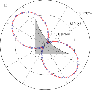
For numerical computation we choose a completely chaotic Sinai billiard, defined as an area between the coordinate axes and the circle where , shown as a shaded area in figure 2a.
We shall consider four different drivings and test the validity of (40), which describes the time evolution of the second moment of the energy fluctuations.
The first example of the driving is a nonuniform rotation where the angle of the billiard changes with time as . According to (13) in this case , and . For large velocities if we can neglect terms involving and the equation (41) gives for the time evolution of the variance of energy fluctuations
| (56) |
We took initial conditions at three different initial velocities , at initial time and uniformly distributed on the remaining 3D phase space. Theoretical prediction (56) agrees with numerical results very well as shown in figure 1a. In all cases is approximately the same , as determined by the fitting procedure, thus it is indeed independent of the velocity. At large times we observe Fermi acceleration with as discussed below.
The second example of the driving is a composition of scaling and rotation in such a way that that the angular momentum of the billiard is preserved (). The angular velocity is and , such that and . In this case we use the equation (42). From (13) we find
| (57) |
which is used in (42) leading to
| (58) |
The analytical expression of this integral is too complicated to be shown here, and it was evaluated numerically in practice as well. We took initial conditions at three different initial velocities , at initial time and uniformly distributed on the remaining 3D phase space. A very good agreement with the theory is found as shown in figure 1b. In all cases is approximately the same , as determined by the fitting procedure, thus it is indeed independent of the velocity. At large times we observe Fermi acceleration with as discussed below.
We used the third driving to find the tensor defined in (39). We translate the billiard back and forth as in 20 different directions spanning from to . According to (42) we have
| (59) |
where
| (60) |
An ensemble of initial conditions at and , uniformly distributed on the remaining phase space, evolved one period in time, was used to determine the evolution of . Measurements of are shown as small circles in a polar plot in figure 2a. Because of the symmetries of the billiard, tensor must be of the form
| (61) |
and
| (62) |
Values of and were found by the best fit procedure. In figure 2a we see that this model describes data very well.
The last example of the driving is a circular translation of the center of mass of the billiard where , and . Although the centre of mass of the billiard is rotating around the origin of the coordinate system, the billiard plane is not rotating, so the angular momentum of the billiard is zero and thus and we expect a slower diffusion. From (42) and (61) we have
| (63) |
We took initial conditions at three different initial velocities , at initial time and uniformly distributed on the remaining 3D phase space. Now without any fit, using the values of and computed previously, we find a very good agreement with the numerical results as shown in figure 2b.

Finally we calculated the acceleration exponents. We took two different drivings. One is a nonuniform rotation with and the other is a translation with . In the case of rotation and we expect asymptotically , while in the case of translations and we expect asymptotically . Numerical results shown in figure 3 confirm the expectations very well. Additionally, we can see the transient regimes where is different from asymptotic values. For small enough velocities we observe the regime where . This is because when the velocity is small the billiard undergoes many oscillations between the collisions and the successive velocity changes are effectively uncorrelated, leading to the random walk like process. In the rotating case we see that after the random walk like phase the system enters the intermediate regime where , which is because the asymptotically big term is still much smaller than , regarding the equation (35). Eventually, for , becomes as predicted by the theory.
Finally, we should add that numerical calculations have been performed for various uniformly rotating billiards (Sinai billiard, elliptical billiard, Robnik billiard Robnik (1983), oval billiard Leonel et al. (2009)) and the conservation law (29) has been confirmed in double precision accuracy, which implies .
VIII Conclusions
In time-dependent fully chaotic shape-preserving billiards the velocity dynamics is determined by the rotational properties of the billiard. If the transformation is such that the angular momentum of the billiard is preserved then the acceleration exponent is , except in the case where the only transformation is a uniform rotation and there is no acceleration, . On the other hand, if the transformation is such that the angular momentum of the billiard is not preserved then the acceleration exponent equals . These three values of exhaust all possible values of the acceleration exponent in fully chaotic time-dependent billiards. However, if the structure of the phase space is more complicated, with the coexisting islands of regular motion, the acceleration exponents may differ from the prediction of the theory presented in this paper, simply because the assumption for the autocorrelation functions (37), (38) and (39) are not fulfilled. In this work we address only the fully chaotic billiards, while the results for the integrable ellipse and mixed type billiards in this context will be published elsewhere. The theory presented in this work complements the other more general theories of the velocity dynamics in time-dependent billiards Karlis et al. (2012); Gelfreich and Turaev (2008).
Acknowledgement
I would like to thank Prof. Marko Robnik for a careful reading and great help in improving the quality of the paper. This work was supported by the Slovenian Research Agency (ARRS).
References
- Stöckmann (1999) H.-J. Stöckmann, Quantum Chaos - An Introduction (Cambridge: Cambridge University Press, 1999).
- Fermi (1949) E. Fermi, Phys. Rev. 75, 1169 (1949).
- Ulam (1961) S. M. Ulam, in Proc. Fourth Berkeley Symp. on Math. Statist. and Prob., Vol. 3, edited by J. Neyman (Univ. of Calif. Press, 1961) pp. 315–320.
- Lieberman and Lichtenberg (1972) M. A. Lieberman and A. J. Lichtenberg, Phys. Rev. A 5, 1852 (1972).
- Gelfreich and Turaev (2008) V. Gelfreich and D. Turaev, J. Phys. A 41, 212003 (2008).
- Gelfreich et al. (2012) V. Gelfreich, V. Rom-Kedar, and D. Turaev, Chaos: An Interdisciplinary Journal of Nonlinear Science 22, 033116 (2012).
- Leonel et al. (2009) E. D. Leonel, D. F. M. Oliveira, and A. Loskutov, Chaos 19, 033142 (2009).
- Shah (2013) K. Shah, Phys. Rev. E 88, 024902 (2013).
- Gelfreich et al. (2013) V. Gelfreich, V. Rom-Kedar, and D. Turaev, (2013), arXiv:1305.2624.
- Lenz et al. (2009) F. Lenz, C. Petri, F. R. N. Koch, F. K. Diakonos, and P. Schmelcher, New J. Phys. 11, 083035 (2009).
- Lenz et al. (2010) F. Lenz, C. Petri, F. K. Diakonos, and P. Schmelcher, Phys. Rev. E (3) 82, 016206 (2010).
- Oliveira and Robnik (2011) D. F. M. Oliveira and M. Robnik, Phys. Rev. E 83, 026202 (2011).
- Batistić and Robnik (2011) B. Batistić and M. Robnik, J. Phys. A 44, 365101, 21 (2011).
- Batistić and Robnik (2012) B. Batistić and M. Robnik, in Let’s face chaos through nonlinear dynamics, AIP Conference Proceedings, Vol. 1468 (2012).
- Loskutov et al. (1999) A. Loskutov, A. Ryabov, and L. Akinshin, J. Exp. Theor. Phys. 89, 966 (1999).
- Hertz (1910) P. Hertz, Annalen der Physik 33, 225 (1910).
- Einstein (1911) A. Einstein, Annalen der Physik 34, 175 (1911).
- de Carvalho et al. (2006) R. E. de Carvalho, F. C. Souza, and E. D. Leonel, Phys. Rev. E 73, 066229 (2006).
- Kamphorst et al. (2007) S. O. Kamphorst, E. D. Leonel, and J. K. L. da Silva, J. Phys. A: Math. Theor. 40, F887 (2007).
- Oliveira and M. (2012) D. F. M. Oliveira and R. M., Int. J. Bifur. Chaos 22, 1250207 (2012).
- Robnik (1983) M. Robnik, J. Phys. A: Math. Gen. 16, 3971 (1983).
- Karlis et al. (2012) A. K. Karlis, F. K. Diakonos, and V. Constantoudis, Chaos 22, 026120 (2012).