Optical Spectroscopy and Velocity Dispersions
of Galaxy Clusters from the SPT-SZ Survey

Abstract

We present optical spectroscopy of galaxies in clusters detected through the Sunyaev-Zel’dovich (SZ) effect with the South Pole Telescope (SPT). We report our own measurements of $61$ spectroscopic cluster redshifts, and $48$ velocity dispersions each calculated with more than $15$ member galaxies. This catalog also includes $19$ dispersions of SPT-observed clusters previously reported in the literature. The majority of the clusters in this paper are SPT-discovered; of these, most have been previously reported in other SPT cluster catalogs, and five are reported here as SPT discoveries for the first time. By performing a resampling analysis of galaxy velocities, we find that unbiased velocity dispersions can be obtained from a relatively small number of member galaxies ($\lesssim 30$), but with increased systematic scatter. We use this analysis to determine statistical confidence intervals that include the effect of membership selection. We fit scaling relations between the observed cluster velocity dispersions and mass estimates from SZ and X-ray observables. In both cases, the results are consistent with the scaling relation between velocity dispersion and mass expected from dark-matter simulations. We measure a $\sim$30% log-normal scatter in dispersion at fixed mass, and a $\sim$10% offset in the normalization of the dispersion-mass relation when compared to the expectation from simulations, which is within the expected level of systematic uncertainty.

1. Introduction

Clusters of galaxies cause a distortion in the cosmic microwave background (CMB) from the inverse Compton scattering of the CMB photons with the hot intra-cluster gas, commonly called the Sunyaev-Zel’dovich (SZ) effect (Sunyaev & Zel’dovich, 1972). SZ cluster surveys efficiently find massive, high-redshift clusters, primarily due to the redshift independence of the brightness of the SZ effect, with completed SZ surveys by the South Pole Telescope (SPT), Atacama Cosmology Telescope (ACT), and Planck having identified over 1000 clusters by their SZ distortion (see, e.g., Staniszewski et al., 2009; Vanderlinde et al., 2010; Williamson et al., 2011; Reichardt et al., 2013; Marriage et al., 2011; Hasselfield et al., 2013; Planck Collaboration et al., 2011, 2013). SZ-selected samples have provided a unique window into high-redshfit cluster evolution (see, e.g., McDonald et al., 2012, 2013; Bayliss et al., 2013), and have also been used to constrain cosmological parameters (see, e.g., Benson et al., 2013; Reichardt et al., 2013).

In this paper, we report spectroscopic observations of galaxies associated with 61 galaxy clusters detected in the 2500 deg² SPT-SZ survey. This work is focused on measuring spectroscopic redshifts, which can inform cosmological studies in two ways. First, we present spectroscopically determined cosmological redshifts for most clusters. The measured spectroscopic redshifts are useful as a training set for photometric redshift measurements (High et al., 2010; Song et al., 2012).

Second, we present velocity dispersions, which are a potentially useful observable for measuring cluster mass (White et al., 2010; Saro et al., 2013). The cosmological constraints from the SPT-SZ cluster survey are currently limited by the uncertainty in the normalization of the SZ-mass relation (Benson et al., 2013; Reichardt et al., 2013). This motivates using multiple mass estimation methods, ideally in a joint likelihood analysis. Our group is pursuing X-ray observations (Andersson et al., 2011), weak lensing (High et al., 2012), and velocity dispersions to address the cluster mass calibration challenge. Currently, the relationship between the SZ observable and mass is primarily calibrated in a joint fit of SZ and X-ray data to a model that includes cosmological and scaling relation parameters (Benson et al., 2013). Like the SZ effect, X-ray emission is produced by the hot gas component of the cluster, so velocity dispersions and weak lensing are important for assessing any systematic biases from gas-based proxies. Velocity dispersions also have the advantage of being obtainable from ground-based telescopes up to high redshift.

The velocities of SPT cluster galaxies presented here are primarily derived from our spectroscopic measurements of 61 massive galaxy clusters. These data are used to produce $48$ velocity dispersions for clusters with more than $15$ member galaxies, several of which we have already presented elsewhere (Brodwin et al., 2010; Foley et al., 2011; Williamson et al., 2011; McDonald et al., 2012; Stalder et al., 2013; Reichardt et al., 2013; Bayliss et al., 2013). These are, for the most part, the data obtained through 2011 in our ongoing spectroscopy program. We also list dispersions collected from the literature, including observations of 14 clusters that were also detected by ACT and targeted for spectroscopic followup by the ACT collaboration (Sifón et al., 2013).

This paper is organized as follows. We describe the observations and observing strategy in Section 2. In Section 3, we present our results, including the individual galaxy velocities and cluster velocity dispersions, and we investigate the phase-space galaxy selection using a stacking analysis. In Section 4, we use a resampling analysis to calculate cluster redshift and dispersion uncertainties that take the effect of the membership selection into account. We explore the properties of our sample of velocity dispersions by comparing them with SZ-based SPT masses, X-ray temperatures, and X-ray-derived masses in Section 5. The evaluation of our observing strategy and outstanding questions are summarized in the conclusion, Section 6.

Throughout this paper, we define $M_{500c}$ ($M_{200c}$) as the mass contained within $R_{500c}$ ($R_{200c}$), the radius from the cluster center within which the average density is 500 (200) times the critical density at the cluster redshift. Conversion between $M_{500c}$ and $M_{200c}$ is made assuming an NFW density profile and the Duffy et al. (2008) mass-concentration relation. We report uncertainties at the 68% confidence level, and we adopt a WMAP7$+$BAO$+H_{0}$ flat $\Lambda$CDM cosmology with $\Omega_{M}=0.272$, $\Omega_{\Lambda}=0.728$, and $H_{0}=70.2~{}$km s^-1 Mpc^-1 (Komatsu et al., 2011).

2. Observations

2.1. South Pole Telescope

Most of the galaxy clusters for which we report spectroscopic observations were published as SPT cluster detections (and new discoveries) in Vanderlinde et al. (2010), Williamson et al. (2011), and Reichardt et al. (2013); we refer the reader to those publications for details of the SPT observations. In Table 2.1, we give the SPT identification (ID) of the clusters and their essential SZ properties. This includes the right ascension and declination of the SZ center, the cluster redshift, and the SPT detection significance $\xi$. We also report the SPT cluster mass estimate, $M_{500c,\mathrm{SPT}}$, as reported in Reichardt et al. (2013), for those clusters at redshift $z\geq 0.3$, the redshift threshold used in the SPT cosmological analysis. As described in Reichardt et al. (2013), the SPT mass estimate is measured from the SPT SZ significance and X-ray measurements, where available, while accounting for the SPT selection, and marginalizing over all uncertainties in cosmology and the cluster observable scaling relations. The last columns indicate the source of the spectroscopy, our own measurements for 61 clusters, and a literature reference for 19 of them. Five clusters have data from both sources.

There are $11$ clusters that do not appear in prior SPT publications, and are presented here as SPT detections for the first time. Five of them are new discoveries (identified with * in Table 2.1), and the other six were previously published as ACT detections (Marriage et al., 2011, identified with ** in Table 2.1). These SPT detections will be reported in an upcoming cluster catalog from the full 2500 deg² SPT-SZ survey.

One cluster, SPT-CL J0245-5302, is detected by SPT at high significance, however because of its proximity to a bright point source ($<8$ arcmin away), it is not included in the official catalog. SPT-CL J2347-5158 had a higher SPT significance in early maps of the survey, but has $\xi<4.0$ in the 2500-deg² survey. The SPT significance and mass are not given for these two clusters.

Table 1SPT properties and source of spectroscopic data

ID & coordinates						Source of spectroscopy
SPT ID	R.A.	Dec.	$z$	$\xi$	$M_{500c,\mathrm{SPT}}$	this work	literature
	(J2000 deg.)	(J2000 deg.)			($10^{14}h_{70}^{-1}M_{\odot}$)
SPT-CL J0000-5748	$0.2496$	$-57.8066$	$0.702$	$5.48$	$4.29\pm 0.71$	✓
SPT-CL J0014-4952*	$3.6969$	$-49.8772$	$0.752$	$8.87$	$5.14\pm 0.86$	✓
SPT-CL J0037-5047*	$9.4441$	$-50.7971$	$1.026$	$6.93$	$3.64\pm 0.79$	✓
SPT-CL J0040-4407	$10.2048$	$-44.1329$	$0.350$	$19.34$	$10.18\pm 1.32$	✓
SPT-CL J0102-4915	$15.7294$	$-49.2611$	$0.870$	$39.91$	$15.69\pm 1.89$		1
SPT-CL J0118-5156*	$19.5990$	$-51.9434$	$0.705$	$5.97$	$3.39\pm 0.82$	✓
SPT-CL J0205-5829	$31.4437$	$-58.4856$	$1.322$	$10.54$	$4.79\pm 1.00$	✓
SPT-CL J0205-6432	$31.2786$	$-64.5461$	$0.744$	$6.02$	$3.29\pm 0.79$	✓
SPT-CL J0232-5257**	$38.1876$	$-52.9578$	$0.556$	$8.65$	$5.04\pm 0.89$		1
SPT-CL J0233-5819	$38.2561$	$-58.3269$	$0.663$	$6.64$	$3.71\pm 0.86$	✓
SPT-CL J0234-5831	$38.6790$	$-58.5217$	$0.415$	$14.65$	$7.64\pm 1.50$	✓
SPT-CL J0235-5121**	$38.9468$	$-51.3516$	$0.278$	$9.78$	-		1
SPT-CL J0236-4938**	$39.2477$	$-49.6356$	$0.334$	$5.80$	$3.39\pm 0.89$		1
SPT-CL J0240-5946	$40.1620$	$-59.7703$	$0.400$	$9.04$	$5.29\pm 1.07$	✓
SPT-CL J0245-5302	$41.3780$	$-53.0360$	$0.300$	-	-	✓
SPT-CL J0254-5857	$43.5729$	$-58.9526$	$0.437$	$14.42$	$7.46\pm 1.46$	✓
SPT-CL J0257-5732	$44.3516$	$-57.5423$	$0.434$	$5.40$	$3.14\pm 0.86$	✓
SPT-CL J0304-4921**	$46.0619$	$-49.3612$	$0.392$	$12.75$	$7.32\pm 1.04$		1
SPT-CL J0317-5935	$49.3208$	$-59.5856$	$0.469$	$5.91$	$3.46\pm 0.89$	✓
SPT-CL J0328-5541	$52.1663$	$-55.6975$	$0.084$	$7.08$	-		3
SPT-CL J0330-5228**	$52.7287$	$-52.4698$	$0.442$	$11.57$	$6.36\pm 1.00$		1
SPT-CL J0346-5439**	$56.7247$	$-54.6505$	$0.530$	$9.25$	$5.07\pm 0.93$		1
SPT-CL J0431-6126	$67.8393$	$-61.4438$	$0.059$	$6.40$	-		2
SPT-CL J0433-5630	$68.2522$	$-56.5038$	$0.692$	$5.35$	$2.89\pm 0.82$	✓
SPT-CL J0438-5419	$69.5749$	$-54.3212$	$0.422$	$22.88$	$10.82\pm 1.39$	✓	1
SPT-CL J0449-4901*	$72.2742$	$-49.0246$	$0.790$	$8.91$	$4.57\pm 0.86$	✓
SPT-CL J0509-5342	$77.3360$	$-53.7045$	$0.462$	$6.61$	$5.36\pm 0.71$	✓	1
SPT-CL J0511-5154	$77.9202$	$-51.9044$	$0.645$	$5.63$	$3.61\pm 0.96$	✓
SPT-CL J0516-5430	$79.1480$	$-54.5062$	$0.294$	$9.42$	-	✓
SPT-CL J0521-5104	$80.2983$	$-51.0812$	$0.675$	$5.45$	$3.46\pm 0.96$		1
SPT-CL J0528-5300	$82.0173$	$-53.0001$	$0.769$	$5.45$	$3.18\pm 0.61$	✓	1
SPT-CL J0533-5005	$83.3984$	$-50.0918$	$0.881$	$5.59$	$2.68\pm 0.61$	✓
SPT-CL J0534-5937	$83.6018$	$-59.6289$	$0.576$	$4.57$	$2.71\pm 1.00$	✓
SPT-CL J0546-5345	$86.6541$	$-53.7615$	$1.066$	$7.69$	$5.25\pm 0.75$	✓	1
SPT-CL J0551-5709	$87.9016$	$-57.1565$	$0.424$	$6.13$	$3.75\pm 0.54$	✓
SPT-CL J0559-5249	$89.9245$	$-52.8265$	$0.609$	$9.28$	$6.79\pm 0.86$	✓	1
SPT-CL J0658-5556	$104.6317$	$-55.9465$	$0.296$	$39.05$	-		4
SPT-CL J2012-5649	$303.1132$	$-56.8308$	$0.055$	$5.99$	-		2
SPT-CL J2022-6323	$305.5235$	$-63.3973$	$0.383$	$6.58$	$3.82\pm 0.89$	✓
SPT-CL J2032-5627	$308.0800$	$-56.4557$	$0.284$	$8.14$	-	✓
SPT-CL J2040-4451	$310.2468$	$-44.8599$	$1.478$	$6.28$	$3.21\pm 0.79$	✓
SPT-CL J2040-5725	$310.0631$	$-57.4287$	$0.930$	$6.38$	$3.25\pm 0.75$	✓
SPT-CL J2043-5035	$310.8285$	$-50.5929$	$0.723$	$7.81$	$4.71\pm 1.00$	✓
SPT-CL J2056-5459	$314.2199$	$-54.9892$	$0.718$	$6.05$	$3.68\pm 0.89$	✓
SPT-CL J2058-5608	$314.5893$	$-56.1454$	$0.606$	$5.02$	$2.64\pm 0.79$	✓
SPT-CL J2100-4548	$315.0936$	$-45.8057$	$0.712$	$4.84$	$2.71\pm 0.93$	✓
SPT-CL J2104-5224	$316.2283$	$-52.4044$	$0.799$	$5.32$	$3.04\pm 0.89$	✓
SPT-CL J2106-5844	$316.5210$	$-58.7448$	$1.131$	$22.08$	$8.36\pm 1.71$	✓
SPT-CL J2118-5055	$319.7291$	$-50.9329$	$0.625$	$5.62$	$3.43\pm 0.93$	✓
SPT-CL J2124-6124	$321.1488$	$-61.4141$	$0.435$	$8.21$	$4.68\pm 0.96$	✓
SPT-CL J2130-6458	$322.7285$	$-64.9764$	$0.316$	$7.57$	$4.46\pm 0.96$	✓
SPT-CL J2135-5726	$323.9158$	$-57.4415$	$0.427$	$10.43$	$5.68\pm 1.11$	✓
SPT-CL J2136-4704	$324.1175$	$-47.0803$	$0.425$	$6.17$	$4.04\pm 0.96$	✓
SPT-CL J2136-6307	$324.2334$	$-63.1233$	$0.926$	$6.25$	$3.18\pm 0.75$	✓
SPT-CL J2138-6007	$324.5060$	$-60.1324$	$0.319$	$12.64$	$6.75\pm 1.32$	✓
SPT-CL J2145-5644	$326.4694$	$-56.7477$	$0.480$	$12.30$	$6.39\pm 1.25$	✓
SPT-CL J2146-4633	$326.6473$	$-46.5505$	$0.932$	$9.59$	$5.36\pm 1.07$	✓
SPT-CL J2146-4846	$326.5346$	$-48.7774$	$0.623$	$5.88$	$3.64\pm 0.93$	✓
SPT-CL J2148-6116	$327.1798$	$-61.2791$	$0.571$	$7.27$	$4.04\pm 0.89$	✓
SPT-CL J2155-6048	$328.9851$	$-60.8072$	$0.539$	$5.24$	$2.82\pm 0.82$	✓
SPT-CL J2201-5956	$330.4727$	$-59.9473$	$0.098$	$13.99$	-		5
SPT-CL J2248-4431	$342.1907$	$-44.5269$	$0.351$	$42.36$	$17.97\pm 2.18$	✓
SPT-CL J2300-5331	$345.1765$	$-53.5170$	$0.262$	$5.29$	-	✓
SPT-CL J2301-5546	$345.4688$	$-55.7758$	$0.748$	$5.19$	$3.11\pm 0.96$	✓
SPT-CL J2325-4111	$351.3043$	$-41.1959$	$0.358$	$12.50$	$7.29\pm 1.07$	✓
SPT-CL J2331-5051	$352.9584$	$-50.8641$	$0.575$	$8.04$	$5.14\pm 0.71$	✓
SPT-CL J2332-5358	$353.1040$	$-53.9733$	$0.402$	$7.30$	$6.50\pm 0.79$	✓
SPT-CL J2337-5942	$354.3544$	$-59.7052$	$0.776$	$14.94$	$8.14\pm 1.14$	✓
SPT-CL J2341-5119	$355.2994$	$-51.3328$	$1.002$	$9.65$	$5.61\pm 0.82$	✓
SPT-CL J2342-5411	$355.6903$	$-54.1887$	$1.075$	$6.18$	$3.00\pm 0.50$	✓
SPT-CL J2344-4243	$356.1847$	$-42.7209$	$0.595$	$27.44$	$12.50\pm 1.57$	✓
SPT-CL J2347-5158*	$356.9423$	$-51.9766$	$0.869$	-	-	✓
SPT-CL J2351-5452	$357.8877$	$-54.8753$	$0.384$	$4.89$	$3.18\pm 1.04$		6
SPT-CL J2355-5056	$358.9551$	$-50.9367$	$0.320$	$5.89$	$4.07\pm 0.57$	✓
SPT-CL J2359-5009	$359.9208$	$-50.1600$	$0.775$	$6.35$	$3.54\pm 0.54$	✓

Note. — SPT ID of each cluster, right ascension and declination of its SZ center, and redshift $z$ (from Tables 3.2 and 4.1, for reference). Also given are the SPT significance $\xi$ and the SZ-based SPT mass, marginalized over cosmological parameters as in Reichardt et al. (2013), for those clusters at $z\geq 0.3$, except for two, as described in Section 2.1. Clusters marked with ** are reported here as SPT detections for the first time, and those with * are new discoveries.

References. — (1) Sifón et al. (2013); (2) Girardi et al. (1996); (3) Struble & Rood (1999); (4) Barrena et al. (2002); (5) Katgert et al. (1998); (6) Buckley-Geer et al. (2011).

2.2. Optical Spectroscopy

The spectroscopic observations presented in this work are the first of our ongoing follow-up program. The data were taken from 2008 to 2012 using the Gemini Multi Object Spectrograph (GMOS; Hook et al., 2004) on Gemini South, the Focal Reducer and low dispersion Spectrograph (FORS2; Appenzeller et al., 1998) on VLT Antu, the Inamori Magellan Areal Camera and Spectrograph (IMACS; Dressler et al., 2006) on Magellan Baade, and the Low Dispersion Survey Spectrograph (LDSS3; Allington-Smith et al., 1994) on Magellan Clay.

In order to place a large number of slitlets in the central region of the cluster, most of the IMACS observations were conducted with the Gladders Image-Slicing Multi-slit Option (GISMO). GISMO optically remaps the central region of the IMACS field-of-view (roughly $3.5^{\prime}\times 3.2^{\prime}$) to sixteen evenly-spaced regions of the focal plane, allowing for a large density of slitlets in the cluster core while minimizing slit collisions on the CCD.

Details about the observations pertaining to each cluster, including the instrument, optical configuration, number of masks, total exposure time, and measured spectral resolution are listed in Table 2.2.

Optical and infrared follow-up imaging observations of SPT clusters are presented alongside our group’s photometric redshift methodology in High et al. (2010), Song et al. (2012) and Desai et al. (2012). Those photometric redshifts (and in a few cases, spectroscopic redshifts from the literature) were used to guide the design of the spectroscopic observations. Multislit masks were designed using the best imaging available to us, usually a combination of ground-based $griz$ (on Blanco/MOSAIC II, Magellan/IMACS, Magellan/LDSS3, or $BVRI$ on Swope) and Spitzer/IRAC $3.6\mathrm{\mu m}$. In addition, spectroscopic observations at Gemini and VLT were preceded by at least one-band ($r$ or $i$) pre-imaging for relative astrometry, and two-band ($r$ and $i$) pre-imaging for red-sequence target selection in the cases where the existing imaging was not deep enough. The exposure times for this pre-imaging were chosen to reach a magnitude depth for galaxy photometry of $m^{\star}+1$ at $10\sigma$ at the cluster redshift.

In designing the multislit masks, top priority for slit placement was given to bright red-sequence galaxies (the red sequence of SPT clusters is discussed in the context of photometric redshifts in High et al., 2010; Song et al., 2012), as defined by their distance to either a theoretical or an empirically-fit red-sequence model. The details varied depending on the quality of the available imaging, the program and the prioritization weighting scheme of the instrument’s mask-making software. In many of the GISMO observations, blue galaxies were given higher priority than faint red galaxies because, especially at high redshift, they were expected to be more likely to yield a redshift. The results from the different red-sequence weighting schemes are very similar, and few emission lines are found, even at $z\gtrsim 1$ (Brodwin et al., 2010; Foley et al., 2011; Stalder et al., 2013, these articles also provide more details about the red-sequence nature of spectroscopic members). The case of SPT-CL J2040-4451 at $z=1.478$ is different and redshifts were only obtained for emission-line galaxies (Bayliss et al., 2013). In all cases, non-red-sequence objects were used to fill out any remaining space in the mask.

The dispersers and filters, listed in Table 2.2, were chosen (within the uncertainty on the photo-$z$) to obtain low- to medium-resolution spectra covering at least the wavelengths of the main spectral features that we use to identify the galaxy redshifts: [O II] emission, and the Ca II H&K absorption lines and break.

The spectroscopic exposure times (also in Table 2.2) for GMOS and FORS2 observations were chosen to reach $S/N=5$ ($S/N=3$) per spectral element just below the $4000\mathrm{\AA}$ break for a red galaxy of magnitude $m^{\star}+1$ ($m^{\star}+0.5$) at $z<1$ ($z>1$). Under the conditions prevailing at the telescope during classical observing, the exposure times for the Magellan observations were determined by a combination of experience, real-time quick-look reductions, and airmass limitations.

Table 2Observations

SPT ID	$z$	UT Date	Instrument	Disperser/Filter	Masks	$N$	$t_{\mathrm{exp}}$ (h)	Resolution (Å)
SPT-CL J0000-5748	$0.702$	2010 Sep 07	GMOS-S	R150_G5326	2	26	1.33	23.7
SPT-CL J0014-4952	$0.752$	2011 Aug 21	FORS2	GRIS_300I/OG590	2	29	2.83	13.5
SPT-CL J0037-5047	$1.026$	2011 Aug 22	FORS2	GRIS_300I/OG590	2	18	5.00	13.5
SPT-CL J0040-4407	$0.350$	2011 Sep 29	GMOS-S	B600_G5323	2	36	1.17	5.7
SPT-CL J0118-5156	$0.705$	2011 Sep 28	GMOS-S	R400_G5325, N&S	2	14	2.53	9.0
SPT-CL J0205-5829	$1.322$	2011 Sep 25	IMACS	Gri-300-26.7/WB6300-950, f/2	1	9	11.00	5.2
SPT-CL J0205-6432	$0.744$	2011 Sep 30	GMOS-S	R400_G5325, N&S	2	15	2.67	9.0
SPT-CL J0233-5819	$0.664$	2011 Sep 29	GMOS-S	R400_G5325, N&S	1	10	1.33	9.0
SPT-CL J0234-5831	$0.415$	2010 Oct 08	IMACS/GISMO	Gra-300-4.3/Z1-430-675, f/4	1	22	1.50	6.5
SPT-CL J0240-5946	$0.400$	2010 Oct 09	IMACS/GISMO	Gra-300-4.3/Z1-430-675, f/4	1	25	1.00	6.4
SPT-CL J0245-5302	$0.300$	2011 Sep 29	GMOS-S	B600_G5323	2	29	0.83	7.0
SPT-CL J0254-5857	$0.437$	2010 Oct 08	IMACS/GISMO	Gra-300-4.3/Z1-430-675, f/4	1	35	1.50	6.9
SPT-CL J0257-5732	$0.434$	2010 Oct 09	IMACS/GISMO	Gra-300-4.3/Z1-430-675, f/4	1	22	1.50	6.6
SPT-CL J0317-5935	$0.469$	2010 Oct 09	IMACS/GISMO	Gra-300-4.3/Z1-430-675, f/4	1	17	1.63	6.6
SPT-CL J0433-5630	$0.692$	2011 Jan 28	IMACS/GISMO	Gri-300-17.5/Z2-520-775, f/2	1	22	1.00	5.7
SPT-CL J0438-5419	$0.422$	2011 Sep 28	GMOS-S	R400_G5325	1	18	0.75	9.0
SPT-CL J0449-4901	$0.790$	2011 Jan 28	IMACS/GISMO	Gri-300-26.7/WB6300-950, f/2	1	20	1.63	5.6
SPT-CL J0509-5342	$0.462$	2009 Dec 12	GMOS-S	R150_G5326	2	18	1.00	23.7
		2012 Mar 23	FORS2	GRIS_300V/GG435	1	4	2.37	13.7
SPT-CL J0511-5154	$0.645$	2011 Sep 30	GMOS-S	R400_G5325, N&S	2	15	2.67	9.0
SPT-CL J0516-5430	$0.294$	2010 Sep 17	IMACS/GISMO	Gra-300-4.3/Z1-430-675, f/4	2	48	1.67	6.7
SPT-CL J0528-5300	$0.769$	2010 Jan 13	GMOS-S	R150_G5326	2	20	3.00	23.7
SPT-CL J0533-5005	$0.881$	2008 Dec 05	LDSS3	VPH-Red	1	4	0.63	5.4
SPT-CL J0534-5937	$0.576$	2008 Dec 05	LDSS3	VPH-Red	1	3	0.45	5.5
SPT-CL J0546-5345	$1.066$	2010 Feb 11	IMACS/GISMO	Gri-300-26.7/WB6300-950, f/2	1	21	3.00	5.7
SPT-CL J0551-5709	$0.424$	2010 Sep 17	IMACS/GISMO	Gra-300-4.3/Z1-430-675, f/4	2	34	1.42	6.8
SPT-CL J0559-5249	$0.609$	2009 Dec 07	GMOS-S	R150_G5326	2	37	1.33	23.7
SPT-CL J2022-6323	$0.383$	2010 Oct 09	IMACS/GISMO	Gra-300-4.3/Z1-430-675, f/4	1	37	1.17	6.7
SPT-CL J2032-5627	$0.284$	2010 Oct 08	IMACS/GISMO	Gra-300-4.3/Z1-430-675, f/4	1	31	1.17	6.8
SPT-CL J2040-4451	$1.478$	2012 Sep 15	IMACS	Gri-300-26.7, f/2	2	14	11.30	9.3
SPT-CL J2040-5725	$0.930$	2010 Aug 13	IMACS/GISMO	Gri-300-26.7/WB6300-950, f/2	1	5	3.00	5.0
SPT-CL J2043-5035	$0.723$	2011 Aug 27	FORS2	GRIS_300I/OG590	2	21	4.00	13.5
SPT-CL J2056-5459	$0.719$	2010 Aug 14	IMACS/GISMO	Gri-300-26.7/WB6300-950, f/2	1	12	2.00	5.3
SPT-CL J2058-5608	$0.607$	2011 Oct 01	GMOS-S	R400_G5325	2	9	1.67	9.0
SPT-CL J2100-4548	$0.712$	2011 Jul 23	FORS2	GRIS_300I/OG590	2	19	1.50	13.5
SPT-CL J2104-5224	$0.799$	2011 Jul 21	FORS2	GRIS_300I/OG590	2	23	2.83	13.5
SPT-CL J2106-5844	$1.131$	2010 Dec 08	FORS2	GRIS_300I/OG590	1	15	3.00	13.5
		2010 Jun 07	IMACS/GISMO	Gri-300-26.7/WB6300-950, f/2	1	4	8.00	4.5
SPT-CL J2118-5055	$0.625$	2011 May 26	FORS2	GRIS_300I/OG590	2	22	1.33	13.5
		2011 Sep 27	GMOS-S	R400_G5325, N&S	1	3	1.20	9.0
SPT-CL J2124-6124	$0.435$	2009 Sep 25	IMACS/GISMO	Gra-300-4.3/Z1-430-675, f/4	1	24	1.50	7.0
SPT-CL J2130-6458	$0.316$	2010 Sep 17	IMACS/GISMO	Gra-300-4.3/Z1-430-675, f/4	2	47	2.00	7.1
SPT-CL J2135-5726	$0.427$	2010 Sep 16	IMACS/GISMO	Gra-300-4.3/Z1-430-675, f/4	1	33	1.00	6.8
SPT-CL J2136-4704	$0.425$	2011 Sep 29	GMOS-S	R400_G5325	2	24	1.67	9.0
SPT-CL J2136-6307	$0.926$	2010 Aug 14	IMACS/GISMO	Gri-300-26.7/WB6300-950, f/2	1	10	2.00	5.0
SPT-CL J2138-6007	$0.319$	2010 Sep 17	IMACS/GISMO	Gra-300-4.3/Z1-430-675, f/4	1	34	1.50	6.8
SPT-CL J2145-5644	$0.480$	2010 Sep 16	IMACS/GISMO	Gra-300-4.3/Z1-430-675, f/4	2	37	2.92	7.4
SPT-CL J2146-4633	$0.931$	2011 Sep 25	IMACS	Gri-300-26.7/WB6300-950, f/2	1	17	3.00	4.7
SPT-CL J2146-4846	$0.623$	2011 Oct 01	GMOS-S	R400_G5325	2	26	2.33	9.0
SPT-CL J2148-6116	$0.571$	2009 Sep 25	IMACS/GISMO	Gra-300-4.3/Z1-430-675, f/4	1	30	1.50	7.1
SPT-CL J2155-6048	$0.539$	2011 Oct 01	GMOS-S	R400_G5325	2	25	1.50	9.0
SPT-CL J2248-4431	$0.351$	2009 Jul 12	IMACS/GISMO	Gra-300-4.3/Z1-430-675, f/4	1	15	1.33	10.9
SPT-CL J2300-5331	$0.262$	2010 Oct 08	IMACS/GISMO	Gra-300-4.3/Z1-430-675, f/4	1	24	1.00	6.8
SPT-CL J2301-5546	$0.748$	2010 Aug 14	IMACS/GISMO	Gri-300-26.7/WB6300-950, f/2	1	11	2.00	5.4
SPT-CL J2325-4111	$0.358$	2011 Sep 28	GMOS-S	B600_G5323	2	33	1.00	5.7
SPT-CL J2331-5051	$0.575$	2008 Dec 05	LDSS3	VPH-Red	2	6	1.00	5.5
		2010 Sep 09	GMOS-S	R150_G5326	2	28	1.00	23.7
		2010 Oct 09	IMACS/GISMO	Gra-300-4.3/Z2-520-775, f/4	2	62	3.50	6.7
SPT-CL J2332-5358	$0.403$	2009 Jul 12	IMACS/GISMO	Gri-200-15.0/WB5694-9819, f/2	1	24	1.50	18.1
		2010 Sep 05	FORS2	GRIS_300V	2	29	4.38	13.7
SPT-CL J2337-5942	$0.776$	2010 Aug 14	GMOS-S	R150_G5326	2	19	3.00	23.7
SPT-CL J2341-5119	$1.003$	2010 Aug 14	GMOS-S	R150_G5326	2	15	6.00	23.7
SPT-CL J2342-5411	$1.075$	2010 Sep 09	GMOS-S	R150_G5326	1	11	3.00	23.7
SPT-CL J2344-4243	$0.595$	2011 Sep 30	GMOS-S	R400_G5325	2	32	2.33	9.0
SPT-CL J2347-5158	$0.869$	2010 Aug 13	IMACS/GISMO	Gri-300-26.7/WB6300-950, f/2	1	12	2.50	5.0
SPT-CL J2355-5056	$0.320$	2010 Sep 17	IMACS/GISMO	Gra-300-4.3/Z1-430-675, f/4	1	37	1.50	7.0
SPT-CL J2359-5009	$0.775$	2009 Nov 22	GMOS-S	R150_G5326	2	7	1.33	23.7
		2010 Aug 14	IMACS/GISMO	Gri-300-26.7/WB6300-950, f/2	1	22	2.00	5.4

Note. — The instruments used for our observations are IMACS on Magellan Baade, LDSS3 on Magellan Clay, GMOS-S on Gemini South, and FORS2 on VLT Antu. The UT date of observation, details of the configuration and the number of observed multislit masks are given, as well as the number of member redshifts retrieved from the observation ($N\equiv N_{\mathrm{members}}$), and the total spectroscopic exposure time for all masks, $t_{\mathrm{exp}}$, in hours. The spectral resolution is the FWHM of sky lines in Angstroms, measured in the science exposures.

2.2.1 Data Processing

We used the COSMOS reduction package (Kelson, 2003) for CCD reductions of IMACS and LDSS3 data, and standard IRAF routines and XIDL routines for GMOS and FORS2. Flux calibration and telluric line removal were performed using the well-exposed continua of spectrophotometric standard stars (Wade & Horne, 1988; Foley et al., 2003). Wavelength calibration is based on arc lamp exposures, obtained at night in between science exposures in the case of IMACS and LDSS3, and during daytime in the same configuration as for science exposures for GMOS and FORS2. In the case of daytime arc frames, the wavelength calibration was refined using sky lines in the science exposures.

The redshift determination was performed using cross-correlation with the fabtemp97 template in the RVSAO package for IRAF (Kurtz & Mink, 1998) or a proprietary template fitting method using the SDSS DR2 templates, and validated by agreement with visually identified absorption or emission features. A single method was used for each cluster depending on the reduction workflow, and both perform similarly. Comparison between the redshifts obtained from the continuum and emission-line redshifts, when both are available from the same spectrum, shows that the uncertainties on individual redshifts (twice the RVSAO uncertainty, see e.g. Quintana et al., 2000) correctly represent the statistical uncertainty of the fit.

2.3. A few-$N_{\mathrm{members}}$ Spectroscopic Strategy

Modern multi-object spectrographs use slit masks, so that the investment in telescope time is quantized by how many masks are allocated to each cluster. The optimization problem is, therefore, to allocate the observation of $m$ masks across $n$ clusters so as to minimize the uncertainty on the ensemble cluster mass normalization.

We pursue a strategy for spectroscopic observations informed by the expectation (from $N$-body simulations; see e.g. Kasun & Evrard, 2005; White et al., 2010; Saro et al., 2013) that line-of-sight projection effects induce an unavoidable intrinsic scatter of 12% in log dispersion ($\ln\sigma$) at fixed mass, implying a 35% scatter in dynamical mass (Saro et al., 2013, see Equation 15 of the present paper). As this 35% intrinsic scatter needs to be added to the dynamical mass uncertainty of any one cluster, for the purpose of mass calibration, obtaining coarser dispersions on more clusters is more informative than measuring higher-precision velocity dispersions on a few clusters. Considering the results of those simulations and the experience encapsulated in the velocity dispersion literature (e.g. Girardi et al., 1993), we have adopted a target of $N_{\mathrm{members}}\sim 20-30$, where $N_{\mathrm{members}}$ is the number of spectroscopic member galaxies in a cluster. This target range of $N_{\mathrm{members}}$ can be obtained by observing two masks per cluster on the spectrographs available to us. The use of a red-sequence selection to target likely cluster members is a necessary feature of this strategy, as a small number of multislit masks only allows us to target a small fraction of the galaxies in the region of the sky around the SZ center.

In discussions throughout this paper, we often use a $N_{\mathrm{members}}\geq 15$ cut. We note that this number is chosen somewhat arbitrarily for the conservative exclusion of systems with very few members. As we will see in the resampling analysis of Section 4, no special statistical transition happens at $N_{\mathrm{members}}=15$, and dispersions with fewer members could potentially be used for reliable mass estimates.

Recent simulations and our data suggest that this choice of few-member strategy may increase the scatter due to systematics in the measured dispersions. This is discussed in Section 4.1.

3. Results

3.1. Individual Galaxy Redshifts

The full sample of redshifts for both member and non-member galaxies is available in electronic format. In Table 3.1, we present a subset composed of central galaxies, for the 50 clusters where we have the central galaxy redshift. We have visually selected the central galaxy for each cluster to be a large, bright, typically cD-type galaxy that is close to the SZ center and that appears to be central to the distribution of galaxies. For each galaxy, the table lists the SPT ID of the associated cluster, a galaxy ID, right ascension and declination, the redshift and redshift-measurement method, and notable spectral features.

Table 3Galaxy redshifts

Associated SPT ID	Galaxy ID	Galaxy R.A.	Galaxy Dec.	$z$	$z$ method	Spectral features
		(J2000 deg.)	(J2000 deg.)
SPT-CL J0000-5748	J000059.99-574832.7	$0.2500$	$-57.8091$	$0.7007\pm 0.0002$	template	[O II], Ca II H&K
SPT-CL J0037-5047	J003747.30-504718.9	$9.4471$	$-50.7886$	$1.0302\pm 0.0002$	template	Ca II H&K
SPT-CL J0118-5156	J011824.76-515628.6	$19.6032$	$-51.9413$	$0.7021\pm 0.0004$	rvsao-xc	Ca II H&K
SPT-CL J0205-5829	J020548.26-582848.4	$31.4511$	$-58.4801$	$1.3218\pm 0.0002$	rvsao-xc	Ca II H&K
SPT-CL J0205-6432	J020507.83-643226.8	$31.2827$	$-64.5408$	$0.7430\pm 0.0001$	rvsao-xc	Ca II H&K
SPT-CL J0233-5819	J023300.97-581937.0	$38.2540$	$-58.3270$	$0.6600\pm 0.0001$	rvsao-xc	Ca II H&K
SPT-CL J0234-5831	J023442.26-583124.7	$38.6761$	$-58.5235$	$0.4146\pm 0.0001$	rvsao-xc	[O II], Ca II H&K
SPT-CL J0240-5946	J024038.38-594548.5	$40.1599$	$-59.7635$	$0.4027\pm 0.0002$	rvsao-xc	Ca II H&K
SPT-CL J0245-5302	J024524.82-530145.3	$41.3534$	$-53.0293$	$0.3028\pm 0.0001$	rvsao-xc	Ca II H&K
SPT-CL J0254-5857	J025415.47-585710.6	$43.5645$	$-58.9530$	$0.4373\pm 0.0001$	rvsao-xc	Ca II H&K
SPT-CL J0257-5732	J025720.95-573254.0	$44.3373$	$-57.5484$	$0.4329\pm 0.0001$	rvsao-xc	Ca II H&K
SPT-CL J0317-5935	J031715.84-593529.0	$49.3160$	$-59.5914$	$0.4677\pm 0.0001$	rvsao-xc	Ca II H&K
SPT-CL J0433-5630	J043301.03-563109.4	$68.2543$	$-56.5193$	$0.6946\pm 0.0002$	rvsao-xc	Ca II H&K
SPT-CL J0438-5419	J043817.62-541920.6	$69.5734$	$-54.3224$	$0.4217\pm 0.0002$	rvsao-xc	Ca II H&K
SPT-CL J0449-4901	J044904.03-490139.1	$72.2668$	$-49.0275$	$0.7949\pm 0.0002$	rvsao-xc	Ca II H&K
SPT-CL J0509-5342	J050921.37-534212.7	$77.3390$	$-53.7035$	$0.4616\pm 0.0002$	template	[O II], Ca II H&K
SPT-CL J0511-5154	J051142.95-515436.6	$77.9290$	$-51.9102$	$0.6488\pm 0.0002$	rvsao-xc	Ca II H&K
SPT-CL J0516-5430	J051637.33-543001.5	$79.1556$	$-54.5004$	$0.2970\pm 0.0002$	rvsao-xc	Ca II H&K
SPT-CL J0528-5300	J052805.29-525953.1	$82.0220$	$-52.9981$	$0.7670\pm 0.0002$	template	Ca II H&K
SPT-CL J0534-5937	J053430.04-593653.8	$83.6252$	$-59.6150$	$0.5757\pm 0.0002$	rvsao-xc	Ca II H&K
SPT-CL J0551-5709	J055135.58-570828.6	$87.8983$	$-57.1413$	$0.4243\pm 0.0002$	rvsao-xc	Ca II H&K
SPT-CL J0559-5249	J055943.19-524926.2	$89.9300$	$-52.8240$	$0.6104\pm 0.0002$	template	Ca II H&K
SPT-CL J2022-6323	J202209.82-632349.3	$305.5409$	$-63.3970$	$0.3736\pm 0.0001$	rvsao-em	[O II]
SPT-CL J2032-5627	J203214.04-562612.4	$308.0585$	$-56.4368$	$0.2844\pm 0.0002$	rvsao-xc	Ca II H&K
SPT-CL J2043-5035	J204317.52-503531.2	$310.8230$	$-50.5920$	$0.7225\pm 0.0005$	template	Ca II H&K
SPT-CL J2056-5459	J205653.57-545909.1	$314.2232$	$-54.9859$	$0.7151\pm 0.0002$	rvsao-xc	Ca II H&K
SPT-CL J2058-5608	J205822.28-560847.2	$314.5928$	$-56.1465$	$0.6061\pm 0.0002$	rvsao-xc	[O II], Ca II H&K
SPT-CL J2100-4548	J210023.85-454834.6	$315.0994$	$-45.8096$	$0.7148\pm 0.0002$	template	Ca II H&K
SPT-CL J2118-5055	J211853.24-505559.5	$319.7218$	$-50.9332$	$0.6253\pm 0.0002$	template	Ca II H&K
SPT-CL J2124-6124	J212437.81-612427.7	$321.1576$	$-61.4077$	$0.4375\pm 0.0001$	rvsao-xc	Ca II H&K
SPT-CL J2130-6458	J213056.21-645840.4	$322.7342$	$-64.9779$	$0.3161\pm 0.0002$	rvsao-xc	Ca II H&K
SPT-CL J2135-5726	J213537.41-572630.7	$323.9059$	$-57.4419$	$0.4305\pm 0.0002$	rvsao-xc	Ca II H&K
SPT-CL J2136-6307	J213653.72-630651.5	$324.2239$	$-63.1143$	$0.9224\pm 0.0002$	rvsao-xc	Ca II H&K
SPT-CL J2138-6007	J213800.82-600753.8	$324.5034$	$-60.1316$	$0.3212\pm 0.0002$	rvsao-xc	Ca II H&K
SPT-CL J2145-5644	J214551.96-564453.5	$326.4665$	$-56.7482$	$0.4813\pm 0.0003$	rvsao-xc	Ca II H&K
SPT-CL J2146-4633	J214635.34-463301.7	$326.6472$	$-46.5505$	$0.9282\pm 0.0002$	rvsao-xc	Ca II H&K
SPT-CL J2146-4846	J214605.93-484653.3	$326.5247$	$-48.7815$	$0.6177\pm 0.0001$	rvsao-xc	Ca II H&K
SPT-CL J2148-6116	J214838.82-611555.9	$327.1617$	$-61.2655$	$0.5649\pm 0.0002$	rvsao-xc	Ca II H&K
SPT-CL J2155-6048	J215555.46-604902.8	$328.9811$	$-60.8175$	$0.5419\pm 0.0001$	rvsao-xc	Ca II H&K
SPT-CL J2248-4431	J224843.98-443150.8	$342.1833$	$-44.5308$	$0.3482\pm 0.0001$	rvsao-xc	Ca II H&K
SPT-CL J2300-5331	J230039.69-533111.4	$345.1654$	$-53.5198$	$0.2630\pm 0.0002$	rvsao-xc	Ca II H&K
SPT-CL J2325-4111	J232511.70-411213.7	$351.2988$	$-41.2038$	$0.3624\pm 0.0003$	rvsao-xc	Ca II H&K
SPT-CL J2331-5051	J233151.13-505154.1	$352.9631$	$-50.8650$	$0.5786\pm 0.0002$	rvsao-xc	Ca II H&K
SPT-CL J2332-5358	J233227.48-535828.2	$353.1145$	$-53.9745$	$0.4041\pm 0.0002$	rvsao-xc	Ca II H&K
SPT-CL J2337-5942	J233727.52-594204.8	$354.3647$	$-59.7014$	$0.7788\pm 0.0002$	template	Ca II H&K
SPT-CL J2341-5119	J234112.34-511944.9	$355.3015$	$-51.3291$	$1.0050\pm 0.0005$	template	Ca II H&K
SPT-CL J2342-5411	J234245.89-541106.1	$355.6912$	$-54.1850$	$1.0808\pm 0.0003$	template	Ca II H&K
SPT-CL J2344-4243	J234443.90-424312.1	$356.1829$	$-42.7200$	$0.5981\pm 0.0008$	rvsao-em	[O II]
SPT-CL J2355-5056	J235547.48-505540.5	$358.9479$	$-50.9279$	$0.3184\pm 0.0002$	rvsao-xc	Ca II H&K
SPT-CL J2359-5009	J235942.81-501001.7	$359.9284$	$-50.1671$	$0.7709\pm 0.0003$	rvsao-xc	Ca II H&K

Note. — Redshifts of individual galaxies. This is a partial listing, and the full table is available electronically. The entries listed here are the central galaxies, a subset of our observations. For each galaxy, the table lists the SPT ID of the associated cluster, a galaxy ID, right ascension and declination, the redshift $z$ and associated uncertainty, redshift measurement method, and notable spectral features. The labels of the “$z$ method” column are “rvsao-xc” and “rvsao-em”, respectively, for the RVSAO cross-correlation to absorption features and fit to emission lines, and “template” for an in-house template-fitting method using the SDSS DR2 templates.

3.2. Cluster Redshifts and Velocity Dispersions

Table 3.2 lists the cluster redshifts and velocity dispersions measured from the galaxy redshifts.

The cluster redshift $z$ is the biweight average (Beers et al., 1990) of member galaxy redshifts (see below) with an uncertainty given by the standard error, as explained in Section 4.2. Once the cluster redshift is computed, the galaxy proper velocities $v_{i}$ are obtained from their redshifts $z_{i}$ by $v_{i}=c(z_{i}-z)/(1+z)$ (Danese et al., 1980). The velocity dispersion $\sigma_{\mathrm{BI}}$ is the square root of the biweight sample variance of proper velocities, the uncertainty of which we found to be well described by $0.92\sigma_{\mathrm{BI}}/\sqrt{N_{\mathrm{members}}-1}$ when including the effect of membership selection (Section 4.2; see Section 4.1 for the formula of the biweight sample variance). We also report the dispersion $\sigma_{G}$ determined from the gapper estimator, which is a preferred measurement, according to Beers et al. (1990), for those clusters with fewer than $15$ member redshifts.

The cluster redshifts and velocity dispersions are calculated using only galaxies identified as members, where membership is established using iterative $3\sigma$ clipping on the velocities (Yahil & Vidal, 1977; Mamon et al., 2010; Saro et al., 2013). The center at each iteration of $3\sigma$-clipping is the biweight average, and $\sigma$ is calculated from the biweight variance, or the gapper estimator in the case where there are fewer than $15$ members. We do not make a hard velocity cut; the initial estimate of $\sigma$ used in the iterative clipping is determined from the galaxies located within $4000$ km s^-1 of the center, in the rest frame.

Figure 1 shows the velocity histogram for each cluster with 15 members or more, as well as an indication of emission-line objects and our determination of member and non-member galaxies.

Figure 1.— Histograms showing the proper velocities of galaxies selected for each cluster, where colors correspond to: (red) passive galaxies, (blue) emission-line galaxies, and (white) non-members. The central galaxy proper velocity is marked with a dotted line, though we note that this was not measured for six clusters, mostly at high redshift ($z\gtrsim 0.8$).

Some entries in Table 3.2 have a star-shaped flag $\star$ in the SPT ID column, which highlights possibly less reliable dispersion measurements. These include $8$ clusters that have fewer than $15$ measured member redshifts, as well as SPT-CL J0205-6432 with $N_{\mathrm{members}}=15$, for which the gapper and biweight dispersions differ by more than one sigma. Since these are not independent measurements but rather two estimates of the same quantity from the same data, we consider a one-sigma discrepancy to be large and an indication that the sampling is inadequate.

Table 4Cluster redshifts and velocity dispersions

SPT ID (and flag)	$N$	$a$	$z$	$\sigma_{\mathrm{SPT}}$	$\sigma_{\mathrm{G}}$	$\sigma_{\mathrm{BI}}$
		($R_{200c,\mathrm{SPT}}$)		(km s-1)	(km s-1)	(km s-1)
SPT-CL J0000-5748	$26$	$1.0$	$0.7019(06)$	$935$	$598\pm 109$	$563\pm 104$
SPT-CL J0014-4952	$29$	$1.3$	$0.7520(09)$	$1004$	$812\pm 140$	$811\pm 141$
SPT-CL J0037-5047	$18$	$1.6$	$1.0262(09)$	$945$	$550\pm 121$	$555\pm 124$
SPT-CL J0040-4407	$36$	$0.4$	$0.3498(10)$	$1171$	$1275\pm 196$	$1277\pm 199$
SPT-CL J0118-5156$\star$	$14$	$0.9$	$0.7050(14)$	$865$	$948\pm 239$	$986\pm 252$
SPT-CL J0205-5829	$9$	$1.3$	$1.3219(16)$	$1101$	-	-
SPT-CL J0205-6432$\star$	$15$	$1.1$	$0.7436(10)$	$862$	$687\pm 167$	$340\pm 84$
SPT-CL J0233-5819$\star$	$10$	$0.9$	$0.6635(14)$	$884$	$783\pm 238$	$800\pm 245$
SPT-CL J0234-5831	$22$	$0.3$	$0.4149(09)$	$1076$	$929\pm 185$	$926\pm 186$
SPT-CL J0240-5946	$25$	$0.4$	$0.4004(09)$	$948$	$999\pm 186$	$1014\pm 190$
SPT-CL J0245-5302	$30$	-	$0.3001(10)$	-	$1245\pm 210$	$1235\pm 211$
SPT-CL J0254-5857	$35$	$0.4$	$0.4371(12)$	$1071$	$1431\pm 223$	$1483\pm 234$
SPT-CL J0257-5732	$23$	$0.6$	$0.4337(12)$	$800$	$1220\pm 237$	$1157\pm 227$
SPT-CL J0317-5935	$17$	$0.5$	$0.4691(06)$	$832$	$473\pm 108$	$473\pm 109$
SPT-CL J0433-5630	$23$	$0.7$	$0.6919(15)$	$817$	$1260\pm 244$	$1232\pm 242$
SPT-CL J0438-5419	$18$	$0.5$	$0.4223(16)$	$1211$	$1428\pm 315$	$1422\pm 317$
SPT-CL J0449-4901	$20$	$0.6$	$0.7898(15)$	$972$	$1067\pm 223$	$1090\pm 230$
SPT-CL J0509-5342	$21$	$0.8$	$0.4616(07)$	$963$	$670\pm 136$	$678\pm 139$
SPT-CL J0511-5154	$15$	$0.9$	$0.6447(11)$	$873$	$778\pm 189$	$791\pm 194$
SPT-CL J0516-5430	$48$	$0.4$	$0.2940(05)$	$995$	$721\pm 96$	$724\pm 97$
SPT-CL J0528-5300	$21$	$1.2$	$0.7694(17)$	$857$	$1397\pm 284$	$1318\pm 271$
SPT-CL J0533-5005	$4$	$0.4$	$0.8813(04)$	$826$	-	-
SPT-CL J0534-5937	$3$	$0.4$	$0.5757(04)$	$782$	-	-
SPT-CL J0546-5345	$21$	$0.8$	$1.0661(18)$	$1080$	$1162\pm 236$	$1191\pm 245$
SPT-CL J0551-5709	$34$	$0.7$	$0.4243(08)$	$848$	$962\pm 152$	$966\pm 155$
SPT-CL J0559-5249	$37$	$0.8$	$0.6092(10)$	$1072$	$1135\pm 172$	$1146\pm 176$
SPT-CL J2022-6323	$37$	$0.4$	$0.3832(08)$	$847$	$1076\pm 163$	$1080\pm 166$
SPT-CL J2032-5627	$31$	$0.3$	$0.2841(06)$	$898$	$771\pm 128$	$777\pm 131$
SPT-CL J2040-4451$\star$	$14$	$1.5$	$1.4780(25)$	$989$	$1111\pm 280$	$676\pm 173$
SPT-CL J2040-5725	$5$	$0.9$	$0.9295(36)$	$890$	-	-
SPT-CL J2043-5035	$21$	$1.1$	$0.7234(07)$	$969$	$509\pm 104$	$524\pm 108$
SPT-CL J2056-5459$\star$	$12$	$0.7$	$0.7185(12)$	$891$	$704\pm 193$	$642\pm 178$
SPT-CL J2058-5608	$9$	$0.9$	$0.6065(18)$	$780$	-	-
SPT-CL J2100-4548	$20$	$1.4$	$0.7121(11)$	$803$	$874\pm 183$	$854\pm 180$
SPT-CL J2104-5224	$23$	$1.5$	$0.7990(14)$	$849$	$1176\pm 228$	$1153\pm 226$
SPT-CL J2106-5844	$18$	$1.0$	$1.1312(21)$	$1287$	$1216\pm 268$	$1228\pm 274$
SPT-CL J2118-5055	$25$	$1.2$	$0.6249(11)$	$855$	$981\pm 182$	$982\pm 184$
SPT-CL J2124-6124	$24$	$0.6$	$0.4354(11)$	$916$	$1151\pm 218$	$1153\pm 221$
SPT-CL J2130-6458	$47$	$0.5$	$0.3164(06)$	$882$	$897\pm 120$	$903\pm 122$
SPT-CL J2135-5726	$33$	$0.4$	$0.4269(09)$	$976$	$1020\pm 164$	$1029\pm 167$
SPT-CL J2136-4704	$24$	$0.6$	$0.4247(14)$	$870$	$1461\pm 277$	$1461\pm 280$
SPT-CL J2136-6307$\star$	$10$	$0.8$	$0.9258(25)$	$883$	$1244\pm 377$	$1269\pm 389$
SPT-CL J2138-6007	$34$	$0.3$	$0.3185(10)$	$1014$	$1269\pm 201$	$1303\pm 209$
SPT-CL J2145-5644	$37$	$0.5$	$0.4798(13)$	$1025$	$1634\pm 248$	$1638\pm 251$
SPT-CL J2146-4633	$18$	$1.0$	$0.9318(28)$	$1057$	$1840\pm 406$	$1817\pm 405$
SPT-CL J2146-4846	$26$	$0.9$	$0.6230(08)$	$872$	$772\pm 140$	$784\pm 144$
SPT-CL J2148-6116	$30$	$0.6$	$0.5707(09)$	$894$	$969\pm 164$	$966\pm 165$
SPT-CL J2155-6048	$25$	$0.9$	$0.5393(12)$	$787$	$1157\pm 215$	$1162\pm 218$
SPT-CL J2248-4431	$15$	$0.2$	$0.3512(15)$	$1417$	$1304\pm 317$	$1301\pm 320$
SPT-CL J2300-5331	$24$	$0.3$	$0.2623(08)$	$816$	$887\pm 168$	$920\pm 177$
SPT-CL J2301-5546$\star$	$11$	$0.7$	$0.7479(22)$	$847$	$1242\pm 357$	$1261\pm 367$
SPT-CL J2325-4111	$33$	$0.6$	$0.3579(15)$	$1048$	$1926\pm 310$	$1921\pm 312$
SPT-CL J2331-5051	$78$	$0.9$	$0.5748(08)$	$970$	$1363\pm 141$	$1382\pm 145$
SPT-CL J2332-5358	$53$	$0.6$	$0.4020(08)$	$1016$	$1253\pm 158$	$1240\pm 158$
SPT-CL J2337-5942	$19$	$0.9$	$0.7764(10)$	$1181$	$700\pm 150$	$707\pm 153$
SPT-CL J2341-5119	$15$	$1.1$	$1.0025(17)$	$1091$	$1111\pm 270$	$959\pm 236$
SPT-CL J2342-5411$\star$	$11$	$1.5$	$1.0746(27)$	$893$	$1278\pm 368$	$1268\pm 369$
SPT-CL J2344-4243	$32$	$0.7$	$0.5952(18)$	$1317$	$1824\pm 298$	$1878\pm 310$
SPT-CL J2347-5158$\star$	$12$	-	$0.8693(11)$	-	$630\pm 173$	$635\pm 176$
SPT-CL J2355-5056	$37$	$0.5$	$0.3200(08)$	$856$	$1124\pm 170$	$1104\pm 169$
SPT-CL J2359-5009	$26$	$0.9$	$0.7747(11)$	$889$	$951\pm 173$

Note. — This table shows the number $N$ ($\equiv N_{\mathrm{members}}$) of spectroscopic members as determined by iterative $3\sigma$ clipping, the aperture radius $a$ within which they were sampled in units of $R_{200c,\mathrm{SPT}}$, the robust biweight average redshift $z$ with the uncertainty in the last two digits in parentheses, the “equivalent dispersion” calculated from the SZ-based SPT mass $\sigma_{\mathrm{SPT}}$ (see Section 3.2.1), and the measured gapper scale $\sigma_{\mathrm{G}}$ and biweight dispersion $\sigma_{\mathrm{BI}}$. The star flag $\star$ in the SPT ID column indicates potentially less reliable dispersion measurements (see Section 3.2).

3.2.1 The Stacked Cluster

To examine the ensemble phase-space galaxy selection, we produce a stacked cluster from our observations; this stacked cluster will also be useful for evaluating our confidence intervals via resampling (see Section 4.2). We generate it in a way that is independent of cluster membership determination. As the calculation of the velocity dispersion and membership selection are unavoidably intertwined, we use the SPT mass — the other uniform mass measurement that we have for all clusters — to normalize the velocities before stacking.

We make a stacked proper-velocity distribution independent of any measurement of the velocity dispersion by calculating the “equivalent dispersion” from the SPT mass. We convert the $M_{500c,\mathrm{SPT}}$ to $M_{200c,\mathrm{SPT}}$ assuming an NFW profile and the Duffy et al. (2008) concentration, and then convert the $M_{200c,\mathrm{SPT}}$ to a $\sigma_{\mathrm{SPT}}$ (in km s^-1) using the Saro et al. (2013) scaling relation. This $\sigma_{\mathrm{SPT}}$ is listed in Table 3.2 for reference. We also normalize the distance to the SZ center by $R_{200c,\mathrm{SPT}}$. The resulting phase-space diagram of the normalized proper velocities $v_{i}/\sigma_{\mathrm{SPT}}$ vs $r_{i}/R_{200c,\mathrm{SPT}}$ is shown in Figure 2. For reference, different velocity cuts are plotted. The black dashed line is a $3\sigma$ cut. The blue dotted line is a radially-dependent $2.7\sigma(R)$ cut, where again the $\sigma(R)$ is from an NFW profile; this velocity cut is found to be optimal for rejecting interlopers by Mamon et al. (2010) (although when considering systems without red-sequence selection). While $3\sigma$ clipping was a natural choice of membership selection algorithm (given our sometimes small sample size for individual clusters), these different cuts demonstrate that we were generally successful at selecting member galaxies. The histogram of proper velocities is shown in the right panel, together with a Gaussian of mean zero and standard deviation of one. The agreement between the distributions is difficult to quantify due to the expected presence of non-members in the histogram. We will see in Section 5 that we measure a systematic bias in normalization.

Figure 2.— Stacked cluster, constructed using the dispersion equivalent to the SPT mass. Left panel: phase-space diagram of velocities. The black dashed line is a 3-sigma cut, and the blue dotted line is a radially-dependent $2.7\sigma(R)$ cut; see the text, Section 3.2.1 for more details. These cuts would be applied iteratively in membership selection. Right panel: histogram of proper velocities, and Gaussian distribution with a mean of zero, a standard deviation of one, and an area equal to that of the histogram.

3.3. Data in the Literature: Summary and Comparison

Table 4.1 contains spectroscopic redshifts and velocity dispersions from the literature for clusters detected by the SPT. Notably, 14 of these clusters are from Sifón et al. (2013), which presents spectrosopic follow-up of galaxy clusters that were detected by the ACT. Because SPT and ACT are both SZ surveys based in the southern hemisphere, there is some overlap between the galaxy clusters detected with the two telescopes. We independently obtained data for five of the clusters that appear in Sifón et al. (2013), and there is some overlap between the cluster members for which we have measured redshifts. These clusters are of some interest for evaluating our follow-up strategy, because the typical number of SPT-reported member galaxiesper dispersion is 25 (for $N_{\mathrm{members}}\geq 15$), while for the overlapping Sifón et al. (2013) sample it is $55$. All of the overlapping cluster redshifts and dispersions are consistent between our work and Sifón et al. (2013) at the one-sigma level, except for the velocity dispersion of SPT-CL J0528-5300. Its velocity histogram shows extended structure (Figure 1). The galaxies responsible for this extended structure are kept by the membership selection algorithm in this paper, but they were either not observed or not classified as cluster members by Sifón et al. (2013). It is not possible to determine from the data in hand whether this discrepancy is statistical or systematic in origin.

We note that ACT-CL J0616-5227, also studied in Sifón et al. (2013), is seen in SPT maps but is excluded from the survey because of its proximity to a point source.

4. Statistical Methodology in the Few-$N_{\mathrm{members}}$ Regime

In this section, we explore the statistical issues surrounding our obtaining reliable estimates of velocity dispersions and associated confidence intervals. A key element in our approach is “resampling”, in which we extract and analyze subsets of the data, either on a cluster-by-cluster basis, or from the stacked cluster that we constructed from the entire catalog. This allows us to generate large numbers of “pseudo-observations” to address statistical questions where we have too few observations to directly answer.

4.1. Unbiased Estimators

Estimators and confidence intervals for velocity dispersions are discussed in Beers et al. (1990), which the reader is encouraged to review. They present estimators such as the biweight, that are resistant and robust. As we are exploring the properties of the few-$N_{\mathrm{members}}$ regime, we would also like our estimators to be unbiased, meaning that the mean estimate should be independent of the number of points that are sampled.

The first point that we would like to make on the subject is that the biweight dispersion (or more correctly, the associated variance) as presented in Beers et al. (1990), is biased for samples, in the same way that the population variance, $\sum_{i}(v_{i}-\bar{v})^{2}/n$, is biased and the sample variance, $\sum_{i}(v_{i}-\bar{v})^{2}/(n-1)$, is not.

We use the biweight sample variance, which does not suffer from this bias (see, e.g., Mosteller & Tukey, 1977):

$$\sigma_{\mathrm{BI}}^{2}=N_{\mathrm{members}}\frac{\sum_{|u_{i}|<1}(1-u_{i}^{2})^{4}(v_{i}-\bar{v})^{2}}{D(D-1)}$$ (1)

where $v_{i}$ are the proper velocities, $\bar{v}$ their average,

$$D=\sum_{|u_{i}|<1}(1-u_{i}^{2})(1-5u_{i}^{2}),$$ (2)

and $u_{i}$ is the usual biweight weighting

$$u_{i}=\frac{v_{i}-\bar{v}}{9\mathrm{MAD}(v_{i})},$$ (3)

where $\mathrm{MAD}(v_{i})$ is the median absolute deviation of the velocities.

We calculate cluster redshifts using the same biweight average estimator that is presented in Beers et al. (1990). Unlike the more subtle case of the variance, the biweight average is unbiased for all $N_{\mathrm{members}}$.

Table 5Cluster redshifts and velocity dispersions from the literature

SPT / this work				Literature
SPT ID	$N$	$z$	$\sigma_{\mathrm{BI}}$	Lit. ID	$N$	$z$	$\sigma_{\mathrm{BI}}$	Ref.
			(km s-1)				(km s-1)
$z<0.3$
SPT-CL J0235-5121	-	-	-	ACT-CL J0235-5121	$82$	$0.2777\pm 0.0005$	$1063\pm 101$	1
SPT-CL J0328-5541	-	-	-	A3126	$38$	$0.0844$	$1041$	3
SPT-CL J0431-6126	-	-	-	A3266	$132$	$0.0594\pm 0.0003$	$1182^{+100}_{-85}$	2
SPT-CL J0658-5556	-	-	-	1E0657-56	$71$	$0.2958\pm 0.0003$	$1249^{+109}_{-100}$	4
SPT-CL J2012-5649	-	-	-	A3667	$123$	$0.0550\pm 0.0004$	$1208^{+95}_{-84}$	2
SPT-CL J2201-5956	-	-	-	A3827	$22$	$0.0983\pm 0.0010$	$1103^{+252}_{-138}$	5
$z\geq 0.3$
SPT-CL J0102-4915	-	-	-	ACT-CL J0102-4915	$89$	$0.8701\pm 0.0009$	$1321\pm 106$	1
SPT-CL J0232-5257	-	-	-	ACT-CL J0232-5257	$64$	$0.5559\pm 0.0007$	$884\pm 110$	1
SPT-CL J0236-4938	-	-	-	ACT-CL J0237-4939	$65$	$0.3344\pm 0.0007$	$1280\pm 89$	1
SPT-CL J0304-4921	-	-	-	ACT-CL J0304-4921	$71$	$0.3922\pm 0.0007$	$1109\pm 89$	1
SPT-CL J0330-5228	-	-	-	ACT-CL J0330-5227	$71$	$0.4417\pm 0.0008$	$1238\pm 98$	1
SPT-CL J0346-5439	-	-	-	ACT-CL J0346-5438	$88$	$0.5297\pm 0.0007$	$1075\pm 74$	1
SPT-CL J0438-5419	$18$	$0.4223\pm 0.0016$	$1422\pm 317$	ACT-CL J0438-5419	$65$	$0.4214\pm 0.0009$	$1324\pm 105$	1
SPT-CL J0509-5342	$21$	$0.4616\pm 0.0007$	$678\pm 139$	ACT-CL J0509-5341	$76$	$0.4607\pm 0.0005$	$846\pm 111$	1
SPT-CL J0521-5104	-	-	-	ACT-CL J0521-5104	$24$	$0.6755\pm 0.0016$	$1150\pm 163$	1
SPT-CL J0528-5300	$21$	$0.7694\pm 0.0017$	$1318\pm 271$	ACT-CL J0528-5259	$55$	$0.7678\pm 0.0007$	$928\pm 111$	1
SPT-CL J0546-5345	$21$	$1.0661\pm 0.0018$	$1191\pm 245$	ACT-CL J0546-5345	$48$	$1.0663\pm 0.0014$	$1082\pm 187$	1
SPT-CL J0559-5249	$37$	$0.6092\pm 0.0010$	$1146\pm 176$	ACT-CL J0559-5249	$31$	$0.6091\pm 0.0014$	$1219\pm 118$	1
SPT-CL J2351-5452	-	-	-	SCSOJ235138-545253	$30$	$0.3838\pm 0.0008$	$855^{+108}_{-96}$	6

Note. — Number of member-galaxy redshifts $N$ ($\equiv N_{\mathrm{members}}$), cluster redshift and velocity dispersion for clusters found in the literature that are also SPT detections. In the cases where we are presenting our own spectroscopic observations, some of the information from Table 3.2 is repeated in the left half of the present table for reference.

References. — (1) Sifón et al. (2013); (2) Girardi et al. (1996); (3) Struble & Rood (1999, this paper does not contain confidence intervals); (4) Barrena et al. (2002); (5) Katgert et al. (1998); (6) Buckley-Geer et al. (2011).

A second issue related to bias at few $N_{\mathrm{members}}$ is the possibility that the presence of velocity substructure would bias the estimation of the dispersion. We tested whether that was the case by extracting smaller pseudo-observations from the $18$ individual clusters for which we obtained $30$ or more member velocities. We did not use the stacked cluster here as substructure would be lost in the averaging. For each cluster, we randomly drew $1000$ pseudo-observations with $10\leq N_{\mathrm{members}}\leq 25$. The cluster redshift and dispersion from those smaller, random samples was computed and compared to the value that was measured with the full data set.

Figure 3 shows the results of this resampling analysis as a function of $N_{\mathrm{members}}$; the black solid line is the average relative error $\left<(\sigma_{\mathrm{BI}}-\sigma_{\mathrm{pseudo-obs}})/\sigma_{\mathrm{BI}}\right>$ of the sample velocity dispersion of all samples across all clusters, while the colored solid lines depict the average relative error for the individual clusters. The average relative error departs from zero at the percent level. From this, we conclude that the observation of only a small number of velocities per cluster does not introduce significant bias in the measurement of the velocity dispersion for an ensemble of clusters.

However, we see that for some individual clusters that have many measured galaxy velocities, the distribution of velocities is such that measuring fewer members in a pseudo-observation yields, on average, a velocity dispersion that can have several to many percent difference with the one obtained with more members. This is a way in which observing few member galaxies will increase the scatter of observed velocity dispersions at fixed mass. The size of our sample does not allow us to pursue this effect thoroughly, but Figure 3 shows that this systematic increase in the scatter is of order 5%, relative to dispersions computed with more than 30 members. Saro et al. (2013) isolate the scatter that is not due to statistical effects and also find that the scatter due to systematics increases at few-$N_{\mathrm{members}}$ and that this effect is most significant when $N_{\mathrm{members}}$ is less than $\sim 30$.

4.2. Confidence intervals

We now turn to the calculation of the statistical uncertainty on our measured redshifts and velocity dispersions. Beers et al. (1990) describe a number of different ways in which the confidence intervals on biweight estimators can be calculated. They conclude that the statistical jackknife and the statistical bootstrap both yield satisfactory confidence intervals. Broadly speaking, both of these methods estimate the confidence intervals by looking at the internal variability of a sample. The statistical jackknife constructs a confidence interval for an estimate from how much it varies when data points are removed. The bootstrap generates a probability distribution function for the estimate from resampling the observed values with replacement a large number of times, often 1000 or more. The confidence intervals can then be found from the percentiles of this distribution. Many publications after Beers et al. (1990) have chosen the bootstrap; different practices seen in its use, with papers quoting asymmetric confidence intervals and others symmetric ones, have promtped us to inspect our uncertainties carefully.

The reason for using the statistical bootstrap or jackknife is the absence of an analytic expression for the distribution of the errors, given that the source distribution of velocities is unknown, as is the distribution of measured biweight dispersions. We use the stacked cluster as the best model of a cluster with our selection of potential member galaxies. As explained in Section 3.2.1, the availability of SPT masses for all clusters allows us to construct this stacked cluster independently of cluster membership determination or dispersion measurements. We draw a large number of pseudo-observations with replacement from the stacked cluster, perform member selection, and calculate the cluster’s redshift and velocity dispersion from each pseudo-observation. Thus, we generate a probability distribution function for those quantities.

We find that the distribution of the measured cluster redshift is close to a normal distribution whose standard deviation is well described by:

$$\Delta z=\frac{1}{c}\frac{\sigma_{\mathrm{BI}}(1+z)}{\sqrt{N_{\mathrm{members}}}}.$$ (4)

This is the “usual” standard error; the $1/c$ factor converts between velocity and redshift, and the $1+z$ factor is needed because $\sigma_{\mathrm{BI}}$ is defined in the rest frame. At any given $N_{\mathrm{members}}$, the average bootstrap and jackknife uncertainties also reproduce this standard error.

In the case of the velocity dispersion, the bootstrap and jackknife give confidence intervals that are too narrow. Simply put, those estimators use a sample’s internal variability to infer likely properties of the population from which it was drawn. However, the variability is reduced by the membership selection, and the effect of that step is not included in the confidence interval.

The distribution of biweight sample dispersions measured in pseudo-observations after $3\sigma$-clipping membership selection is also observed to be close to a normal distribution in our resampling analysis. We set out to model the standard deviation of this distribution, which is the uncertainty that we are looking for.

If we draw observations from a normal distribution of variance $\sigma^{2}$ and calculate the velocity dispersion as the “usual” (non-biweight) sample standard deviation from $n$ members, without a membership selection step, then the distribution of the measured standard deviation is related to a chi distribution with $n-1$ degrees of freedom. Indeed, the sample standard deviation $s$ is

$$s=\sqrt{\frac{1}{n-1}\sum_{i=1}^{n}(v_{i}-\bar{v}_{i})^{2}}$$ (5)

This implies that

$$\frac{s}{\sigma} = \sqrt{\frac{1}{n-1}\sum_{i=1}^{n}\frac{(v_{i}-\bar{v}_{i})^{2}}{\sigma^{2}}}$$ (6)

$$\Rightarrow\quad\sqrt{n-1}\frac{s}{\sigma} = \sqrt{\sum_{i=1}^{n}\frac{(v_{i}-\bar{v}_{i})^{2}}{\sigma^{2}}}\sim\chi_{n-1}$$ (7)

which is the definition of a chi distribution.

The variance of the chi distribution varies very little between $k=10$ and $k=100$ degrees of freedom:

$$\mathrm{Var}\,\chi_{k} = k-2\left(\frac{\Gamma((k+1)/2)}{\Gamma(k/2)}\right)^{2}$$ (8)

$$= 0.49\quad(k=10)$$ (9)

$$= 0.50\quad(k=100).$$ (10)

Therefore, taking the square root on each side to find the standard deviation $\Delta$ of the dispersion estimate $s$:

$$\Delta(\sqrt{n-1}\frac{s}{\sigma}) = \sqrt{0.5}=0.7$$ (11)

$$\Rightarrow\quad\Delta s = 0.7\sigma/\sqrt{n-1}$$ (12)

Following the above, we model the uncertainty as

$$\Delta\sigma_{\mathrm{BI}} = C_{\mathrm{BI}}\sigma_{\mathrm{BI}}/\sqrt{N_{\mathrm{members}}-1}$$ (13)

where $C_{\mathrm{BI}}$ is a constant. We also parameterize the uncertainty on the gapper measurement in the same way, with a constant $C_{\mathrm{G}}$.

Figure 4 shows the relative error in $\sigma_{\mathrm{BI}}$ measured from the resampling analysis, as a function of $N_{\mathrm{members}}$, for $10\leq N_{\mathrm{members}}\leq 60$. The solid black line shows the average error, and the blue dashed line is the asymmetric root-mean-square error.

We find the numerical value of $C_{\mathrm{BI}}$ as the mean ratio of the RMS error and $1/\sqrt{N_{\mathrm{members}}-1}$. We find that $C_{\mathrm{BI}}=0.92$. The green dotted line of Figure 4 shows the uncertainty given by our model, $\pm 0.92/\sqrt{N_{\mathrm{members}}-1}$. Similarly for the gapper scale, we find that $C_{\mathrm{G}}=0.91$.

Therefore, we find that the 3-$\sigma$ membership selection combined with the biweight estimation of the dispersion gives an uncertainty increased by 30% compared with random sampling from a normal distribution, and also compared to the bootstrap and jackknife estimates. The larger errors are caused by non-Gaussianity in the velocity distribution and by the cluster membership selection, which can both include non-members and reject true members, generically leading to increased scatter in the measured dispersion.

We note that this effect is different than the systematic scatter shown in Figure 3, where the measured dispersion changed significantly for some individual clusters when resampling with fewer galaxy members. This latter effect likely has both physical (e.g., velocity sub-structure in the cluster) and measurement (e.g., member selection, interlopers) origins. However, both effects will be present at some level in any dispersion measurement, and the results here are important benchmarks for simulations to compare to and reproduce.

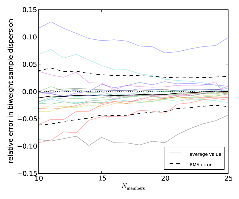
Figure 3.— Average relative error $\left<(\sigma_{\mathrm{BI}}-\sigma_{\mathrm{pseudo-obs}})/\sigma_{\mathrm{BI}}\right>$ in the measured dispersion for pseudo-observations sampled from each individual cluster with more than 30 members, as described in Section 4.1. The colored solid lines show the average across pseudo-observations for each individual cluster. The black solid line is the average across clusters, and the dashed lines show the one-sigma range in the distribution of colored traces. The dotted line is identically zero. 1000 pseudo-observations were drawn with replacement at each $N_{\mathrm{members}}$, and three-sigma clipping membership selection was applied to each pseudo-observation before computation of the dispersion. The average relative error departs from zero at the percent level; from this we conclude that the observation of only a small number of velocities per cluster does not introduce bias in the measurement of the velocity dispersion, in an ensemble sense. However, it presents an additional source of error for individual clusters, which will increase the measurement scatter.

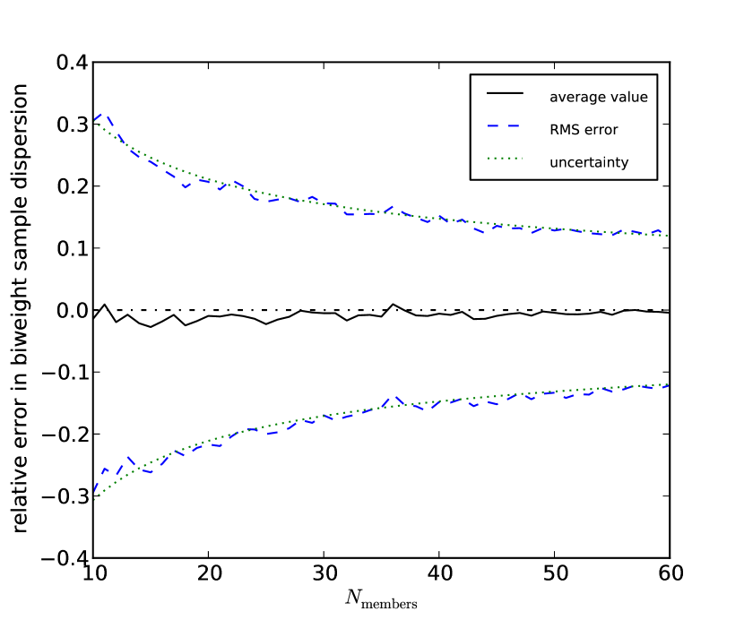
Figure 4.— Statistical uncertainty and relative error in the measured dispersion for pseudo-observations sampled from the stacked cluster, as described in Section 4.2. The black solid line shows the average error, the blue dash-dotted line is the asymmetric root-mean-square error, and the green dotted line is the (relative) uncertainty, $\pm 0.92/\sqrt{N_{\mathrm{members}}-1}$. The parameter $C_{\mathrm{BI}}=0.92$ from Equation 13 was fit using this root-mean-square error, hence the agreement of the lines. The dot-dashed line is identically zero. 1000 pseudo-observations were drawn with replacement at each $N_{\mathrm{members}}$, and three-sigma clipping membership selection was applied to each pseudo-observation before computation of the dispersion.

5. Comparison of Velocity Dispersions with Other Observables

In this section, we compare our cluster velocity dispersion measurements with gas-based observables and estimates of the cluster mass. In particular, we measure the normalization and the scatter of scaling relations between the two observables, and compare these to our expectations from simulations. We neglect effects related to the SZ cluster selection, variation of the cosmology, or potentially correlated intrinsic scatter between observables, and leave the accounting of these effects to future work. However, this comparison is still useful in understanding how our velocity dispersion mass estimates compare to those using other methods, and can also help identify systematics.

5.1. Comparison with SPT Masses

Figure 5.— Cluster biweight velocity dispersions from Table 3.2 as a function of SZ-based SPT masses (Table 2.1, Section 2.1) for clusters with $N_{\mathrm{members}}\geq 15$ and $z\geq 0.3$. The figure also shows the scaling relationship between velocity dispersion and mass expected from dark-matter simulations as a solid line (Saro et al., 2013). The dashed line is this same scaling relationship, shifted to show the average scaling relationship implied by the mean log mass ratio of the data points.

Figure 5 shows 43 cluster biweight velocity dispersions from Table 3.2 plotted against the masses estimated from their SPT SZ signal (combined with X-ray observations where applicable; Table 2.1, Section 2.1). The clusters that are included are those with $N_{\mathrm{members}}\geq 15$ and $z\geq 0.3$, except for SPT-CL J0205-6432, which was flagged as having a potentially less reliable dispersion measurement in Section 3.2. We also plot, as a solid line, the predicted scaling between dispersion and mass from Saro et al. (2013)

$$M_{200c,\,\mathrm{dyn}}=\left(\frac{\sigma_{\mathrm{DM}}}{A\times h_{70}(z)^{C}}\right)^{B}10^{15}M_{\odot}$$ (14)

where $A=939$, $B=2.91$ and $C=0.33$, with negligible statistical uncertainty compared to the systematic uncertainty, whose floor is evaluated to be at 5% in dispersion (Evrard et al., 2008). $\sigma_{\mathrm{DM}}$ is the dispersion computed from dark-matter subhalos, which are identified as galaxies in simulations. This has a different functional form but is consistent with the Evrard et al. (2008) scaling relation.

Our measurements appear to have a systematic offset relative to the model prediction. To quantify this offset, we compute the mean of the log mass ratio, $\ln(M_{200c,\,\mathrm{dyn}}/M_{200c,\,\mathrm{SPT}})$. For each cluster $i$, we compute this log mass ratio, and its associated uncertainty $\sigma_{\ln M_{\mathrm{ratio}},i}$. The uncertainty in the ratio is estimated from the quadrature sum of the fractional uncertainty in the SZ and dynamical mass estimates. To the latter, we add the expected intrinsic scatter in dynamical to true-mass as estimated by Saro et al. (2013):

$$\Delta_{\ln(M_{200c,\,\mathrm{dyn}}/M_{200c})}=0.3+0.075z.$$ (15)

The uncertainty on the SZ-based SPT mass already includes the effect of intrinsic scatter.

The weighted average log mass ratio is

$$\left<\ln(M_{200c,\,\mathrm{dyn}}/M_{200c,\,\mathrm{SPT}})\right>=0.33\pm 0.10,$$ (16)

where the weights for each data point are given by $1/\sigma_{\ln M_{\mathrm{ratio}},i}^{2}$, and the uncertainty on the average is given by $1/\sigma^{2}=\sum_{i}1/\sigma_{\ln M_{\mathrm{ratio}},i}^{2}$. This average log ratio means that the dynamical mass is $\exp(0.33)=1.39$ times the SPT mass estimate.

Figure 5 shows as a dashed blue line how the N-body scaling relation is shifted if the log mass ratio is shifted by $0.33$ to make the mass estimates coincide. Because the slope is $1/B=1/2.91$, the offset in log dispersion is $(0.33\pm 0.10)/2.91=0.11\pm 0.03$. In other words, the measured velocity dispersions are on average $\exp(0.11)=1.12$ times their expected value given the N-body simulation work and the current normalization of the SPT mass estimate. The size of this normalization offset is consistent with the expected size of systematic biases, as discussed in Section 5.3.

We quantify the level of Gaussianity in the dispersion estimates around the best-fit dispersion-mass relation by performing the Anderson-Darling test on the residuals. We find that the residuals are non-Gaussian at the 95% confidence level. If we remove the two clusters with the lowest dispersions (SPT-CL J0317-5935 and SPT-CL J2043-5035), we find per the Anderson-Darling test that the residuals are consistent with a normal distribution. This suggests that the scatter in $\ln\sigma$ is normal – i.e., that the dispersion distribution is log-normal – with a tail towards low dispersion, as might be suspected from the distribution of data points in Figure 5.

If the statistical uncertainty on dispersion measurements of individual clusters has been correctly estimated and is much larger than any systematic uncertainty, then the fractional scatter in $\ln\sigma$ at fixed mass should roughly equal the average fractional uncertainty in the individual measurements. The mean uncertainty in log dispersion at fixed mass is 0.24, including the intrinsic scatter of the scaling relation and the uncertainty on the SPT mass. Analysis of mock observations from simulated clusters indicate that the combination of intrinsic, statistical, and systematic effects would lead to a log-normal scatter of 0.26 in dispersion at fixed mass (Saro et al., 2013). Both numbers are smaller but in general agreement with the measured scatter in $\ln\sigma$ at fixed mass, $(0.31\pm 0.03)$. Systematic effects can increase the scatter, as discussed in Section 5.3.

5.2. Comparison with X-ray Observations

In this section, we compare the velocity dispersion measurements to X-ray observables and mass estimates, and contrast these results with predictions from simulations. We also compare our results to those when using a separate low-redshift sample of comparable-mass clusters with similar velocity dispersion and X-ray observables.

For the clusters in this work, we primarily use X-ray measurements from a Chandra X-ray Visionary Project to observe the 80 most significantly detected clusters by the SPT at $z>0.4$ (PI: B. Benson). This cluster sample has been observed and analyzed in a uniform fashion to derive cluster mass-observables (Benson et al., 2014) and cluster cooling properties (McDonald et al., 2013). In Table 5.2, we give the X-ray measured ICM temperature, $T_{X}$, and the $Y_{X}$-derived cluster mass, $M_{500c,\mathrm{Y_{X}}}$, for the 28 clusters that overlap with the sample from Benson et al. (2014).

We also plot our results alongside velocity dispersion and X-ray measurements of comparable-mass low-redshift clusters taken from the literature. For the X-ray measurements, we use measurements of $T_{X}$ and $M_{500c,\mathrm{Y_{X}}}$ from the low-$z$ sample of Vikhlinin et al. (2009), which were produced following an analysis identical to that used in Benson et al. (2014). The velocity dispersions for many of those galaxy clusters were calculated in a uniform way in Girardi et al. (1996). These velocity dispersion measurements were made with a different galaxy selection and more cluster members, and so will carry different systematics from our own. They nonetheless provide an interesting baseline for comparison. We will see that the scatter of those data points is smaller that that of our sample. Taking instrinsic scatter and mass uncertainties into account, the measured scatter of the literature sample at fixed mass is consistent both with our analysis from Section 4.2 and with the Girardi et al. (1996) uncertainties, and therefore is due to the lower statistical uncertainty.

Figure 6.— Velocity dispersion compared to X-ray properties. The blue points are our sample, and the black crosses are the data from the literature, with X-ray data from Vikhlinin et al. (2009) and dispersions from Girardi et al. (1996); two of them are also low-redshift SPT detections and are circled. Left panel: velocity dispersion vs. X-ray temperature. The dot-dashed line is the best-fit scaling relation from Girardi et al. (1996). The dashed line shows the scaling expected if galaxies and gas were both in equilibrium with the gravitational potential. Right panel: velocity dispersion vs. $M_{500c,\mathrm{Y_{X}}}$. The solid line is the scaling relation from (Saro et al., 2013), and the dashed line is this same scaling relationship, shifted to show the average scaling relationship implied by the mean log mass ratio of the data points.

Table 6X-ray and velocity dispersion data

Cluster ID	$z$	$N$	$\sigma_{\mathrm{BI}}$	$T_{X}$	$M_{500c,\mathrm{Y_{X}}}$
			(km s-1)	(keV)	($10^{14}M_{\odot}$)
SPT-CL
J0000-5748	$0.702$	$26$	$563\pm 104$	$6.75^{+3.09}_{-1.85}$	$4.11^{+1.06}_{-0.80}$
J0014-4952	$0.752$	$29$	$811\pm 141$	$5.91^{+1.09}_{-0.65}$	$4.97^{+0.54}_{-0.38}$
J0037-5047	$1.026$	$18$	$555\pm 124$	$2.85^{+1.44}_{-0.75}$	$1.22^{+0.38}_{-0.28}$
J0040-4407	$0.350$	$36$	$1277\pm 199$	$5.95^{+1.09}_{-0.74}$	$5.42^{+0.62}_{-0.49}$
J0234-5831	$0.415$	$22$	$926\pm 186$	$9.20^{+3.98}_{-2.52}$	$6.83^{+1.62}_{-1.24}$
J0438-5419	$0.422$	$18$	$1422\pm 317$	$11.32^{+2.07}_{-1.76}$	$10.74^{+1.19}_{-1.11}$
J0449-4901	$0.790$	$20$	$1090\pm 230$	$10.39^{+3.43}_{-2.53}$	$6.50^{+1.24}_{-1.08}$
J0509-5342	$0.462$	$21$	$678\pm 139$	$7.28^{+1.30}_{-1.38}$	$5.62^{+0.65}_{-0.72}$
J0516-5430	$0.294$	$48$	$724\pm 97$	$10.95^{+2.27}_{-1.73}$	$12.25^{+1.52}_{-1.31}$
J0528-5300	$0.769$	$21$	$1318\pm 271$	$4.85^{+1.56}_{-0.98}$	$2.68^{+0.50}_{-0.38}$
J0546-5345	$1.066$	$21$	$1191\pm 245$	$7.61^{+2.45}_{-1.52}$	$5.22^{+0.98}_{-0.74}$
J0551-5709	$0.424$	$34$	$966\pm 155$	$3.12^{+0.28}_{-0.28}$	$3.04^{+0.23}_{-0.23}$
J0559-5249	$0.609$	$37$	$1146\pm 176$	$6.74^{+0.76}_{-0.71}$	$5.93^{+0.45}_{-0.45}$
J2043-5035	$0.723$	$21$	$524\pm 108$	$5.87^{+1.03}_{-0.63}$	$4.44^{+0.50}_{-0.38}$
J2106-5844	$1.131$	$18$	$1228\pm 274$	$10.36^{+2.49}_{-1.79}$	$8.37^{+1.26}_{-1.07}$
J2135-5726	$0.427$	$33$	$1029\pm 167$	$7.78^{+4.41}_{-2.10}$	$5.15^{+1.56}_{-0.97}$
J2145-5644	$0.480$	$37$	$1638\pm 251$	$5.34^{+0.90}_{-0.74}$	$5.00^{+0.57}_{-0.52}$
J2148-6116	$0.571$	$30$	$966\pm 165$	$8.24^{+3.14}_{-2.18}$	$5.42^{+1.14}_{-0.93}$
J2248-4431	$0.351$	$15$	$1301\pm 320$	$12.37^{+1.01}_{-0.77}$	$16.35^{+0.84}_{-0.70}$
J2325-4111	$0.358$	$33$	$1921\pm 312$	$8.84^{+2.16}_{-1.55}$	$8.39^{+1.19}_{-0.98}$
J2331-5051	$0.575$	$78$	$1382\pm 145$	$6.38^{+1.84}_{-1.25}$	$4.66^{+0.81}_{-0.66}$
J2332-5358	$0.402$	$53$	$1240\pm 158$	$7.40^{+1.20}_{-0.70}$	$5.66^{+0.48}_{-0.48}$
J2337-5942	$0.776$	$19$	$707\pm 153$	$6.95^{+1.91}_{-1.31}$	$5.76^{+0.92}_{-0.74}$
J2341-5119	$1.002$	$15$	$959\pm 236$	$9.30^{+2.45}_{-2.02}$	$5.77^{+0.89}_{-0.83}$
J2344-4243	$0.595$	$32$	$1878\pm 310$	$11.72^{+2.88}_{-2.10}$	$11.64^{+1.64}_{-1.36}$
J2359-5009	$0.775$	$26$	$950\pm 175$	$4.41^{+1.18}_{-0.65}$	$2.58^{+0.41}_{-0.28}$
Literature
A3571	$0.039$	$70$	$1085^{+110}_{-107}$	$6.81\pm 0.10$	$5.90\pm 0.06$
A2199	$0.030$	$51$	$860^{+134}_{-83}$	$3.99\pm 0.10$	$2.77\pm 0.05$
A496	$0.033$	$151$	$750^{+61}_{-56}$	$4.12\pm 0.07$	$2.96\pm 0.04$
A3667	$0.056$	$123$	$1208^{+95}_{-84}$	$6.33\pm 0.06$	$7.35\pm 0.07$
A754	$0.054$	$83$	$784^{+90}_{-85}$	$8.73\pm 0.00$	$8.47\pm 0.13$
A85	$0.056$	$131$	$1069^{+105}_{-92}$	$6.45\pm 0.10$	$5.98\pm 0.07$
A1795	$0.062$	$87$	$887^{+116}_{-83}$	$6.14\pm 0.10$	$5.46\pm 0.06$
A3558	$0.047$	$206$	$997^{+61}_{-51}$	$4.88\pm 0.10$	$4.78\pm 0.07$
A2256	$0.058$	$47$	$1279^{+136}_{-117}$	$8.37\pm 0.24$	$7.84\pm 0.15$
A3266	$0.060$	$132$	$1182^{+100}_{-85}$	$8.63\pm 0.18$	$9.00\pm 0.13$
A401	$0.074$	$123$	$1142^{+80}_{-70}$	$7.72\pm 0.30$	$8.63\pm 0.24$
A2052	$0.035$	$62$	$679^{+97}_{-59}$	$3.03\pm 0.07$	$1.84\pm 0.03$
Hydra-A	$0.055$	$82$	$614^{+52}_{-43}$	$3.64\pm 0.06$	$2.83\pm 0.03$
A119	$0.044$	$80$	$850^{+108}_{-92}$	$5.72\pm 0.00$	$4.50\pm 0.03$
A2063	$0.034$	$91$	$664^{+50}_{-45}$	$3.57\pm 0.19$	$2.21\pm 0.08$
A1644	$0.048$	$92$	$937^{+107}_{-77}$	$4.61\pm 0.14$	$4.21\pm 0.09$
A3158	$0.058$	$35$	$1046^{+174}_{-99}$	$4.67\pm 0.07$	$4.13\pm 0.05$
MKW3s	$0.045$	$30$	$612^{+69}_{-52}$	$3.03\pm 0.05$	$2.09\pm 0.03$
A3395	$0.051$	$107$	$934^{+123}_{-100}$	$5.10\pm 0.17$	$6.74\pm 0.18$
A399	$0.071$	$92$	$1195^{+94}_{-79}$	$6.49\pm 0.17$	$6.18\pm 0.11$
A576	$0.040$	$48$	$1006^{+138}_{-91}$	$3.68\pm 0.11$	$2.34\pm 0.05$
A2634	$0.030$	$69$	$705^{+97}_{-61}$	$2.96\pm 0.09$	$1.74\pm 0.04$
A3391	$0.055$	$55$	$990^{+254}_{-128}$	$5.39\pm 0.19$	$4.06\pm 0.10$

Note. — SPT data and data from the literature used in Figure 6. For the SPT data, the redshift, number of member-galaxy redshifts $N$ ($\equiv N_{\mathrm{members}}$) and velocity dispersion from Table 3.2 are repeated for reference, and the X-ray temperature and $M_{500c,\mathrm{Y_{X}}}$ are from the same Chandra XVP program, except for one case that are marked. The literature clusters draw their velocity dispersion from Girardi et al. (1996) and X-ray properties from Vikhlinin et al. (2009).

Figure 6 shows the velocity dispersion versus X-ray temperature and versus $M_{500c,\mathrm{Y_{X}}}$. The blue points are our data, and the black crosses are the data from the literature; these literature data are listed for reference in Table 5.2.

The left panel of Figure 6 shows dispersion versus $T_{X}$. The empirical best-fit scaling relation from Girardi et al. (1996), where $\sigma\propto T_{X}^{0.61}$, is plotted as a solid line; this scaling relation is consistent with the Vikhlinin et al. (2009) temperatures used here, although it was fit using X-ray temperatures from a different source, David et al. (1993). The comparison to the temperature is especially interesting in that there is, to first order, a simple correspondence between temperature and velocity dispersion. Assuming that the galaxies and gas are both in equilibrium with the potential (see, e.g., Voit, 2005), then $\sigma^{2}=k_{\mathrm{B}}T_{X}/(\mu m_{p})$, where $m_{p}$ is the proton mass, and $\mu$ the mean molecular weight (we take $\mu=0.58$; see Girardi et al., 1996). This energy equipartition line is plotted as a dashed line in the left panel of Figure 6. Real clusters show a deviation from this simple model, but it offers an interesting theoretical baseline, one independent of data or simulations. This relation implies that the temperature and velocity dispersion have a similar redshift evolution, which is why the quantities in this plot are uncorrected for redshift.

The X-ray $Y_{X}$ observable, while not independent from $T_{X}$, is expected to be significantly less sensitive to cluster mergers than $T_{X}$, with simulations predicting $Y_{X}$ to have both a lower scatter and to be a less biased mass indicator (see, e.g., Kravtsov et al., 2006; Fabjan et al., 2011). For this reason, we also plot the velocity dispersion against $M_{500c,\mathrm{Y_{X}}}$ (times a redshift-evolution factor), in the right panel of Figure 6. The dot-dashed line is the scaling relation predicted from the simulation analysis of Saro et al. (2013).

Computing the average log ratio of the dynamical and $Y_{X}$-based masses gives $0.26\pm 0.12$, corresponding to a bias of $0.09\pm 0.04$ in log dispersion. This was computed, in the previous section, to be $0.33\pm 0.10$ in the case of dynamical and SPT masses, corresponding to $0.11\pm 0.03$ in log dispersion. The residuals of the dispersion-$M_{500c,\mathrm{Y_{X}}}$ relation have a measured scatter in dispersion of $0.31\pm 0.03$, which is the same as the measurement made using the SZ-based SPT mass. The Anderson-Darling test gives similar results to the residuals of the previous section, suggesting a normal scatter in $\ln\sigma$ with a tail towards low dispersion.

While there is very good agreement between the scaling relations comparing the dispersion to the SPT and X-ray mass estimates, we note that the results are not independent. Nine of the clusters included in this work from Reichardt et al. (2013) quoted joint SZ and X-ray mass estimates, which we have included in our sample of SPT mass estimates. In addition, the SPT significance-mass relation used in the SZ mass estimates was in part calibrated from a sub-sample of SPT clusters with X-ray mass estimates, which have effectively calibrated the SPT cluster mass normalization. Regardless, the majority of clusters in this work have SPT mass estimates derived only from the SPT SZ measurements, which have very different noise properties from the X-ray measurements, therefore the agreement in the measured scatters is not entirely trivial.

5.3. Systematics

There are two different, although related, systematics that affect the interpretation of velocity dispersion measurements: systematics that can affect the measurement of the velocity dispersion of galaxies, and a possible velocity bias between the galaxies and the underlying dark matter halo. The velocity bias cannot be empirically measured in our data. However, both effects have been quantified in recent cluster simulation studies (Saro et al., 2013; Gifford et al., 2013; Munari et al., 2013; Wu et al., 2013). In principle, the velocity bias could explain part of the offset between our measurements and the predicted relation from N-body simulations, described in Sections 5.1 and 5.2. The velocity bias has been estimated to be on order of $\sim$5% by Evrard et al. (2008). More recent studies have found a spread in the velocity bias of $\sim$10% when comparing different tracers and algorithms for predicting the galaxy population (Gifford et al., 2013) and comparing dark-matter with hydrodynamic simulations (Munari et al., 2013; Wu et al., 2013).

The measured velocity dispersion can be biased from the true value by the galaxy selection of the measurements, in principle being affected by systematics relating to the luminosity, color, and offset from the cluster center of the galaxies. The observations will also have some amount of imperfect membership determination, due to the presence of interlopers.

Of those effects, the luminosity of the selected galaxies has the potential to create the largest bias, according to recent simulation work showing that brighter galaxies have a smaller velocity dispersion (Saro et al., 2013; Old et al., 2013; Wu et al., 2013; Gifford et al., 2013). Observing only the 25 brightest galaxies of the halo leads to the velocity dispersion being biased low by as much as $\sim$5-10%. These results are difficult to directly compare to our measurements, because the simulated observations use the $N$ brightest galaxies, while real ones target a more varied population. Nonetheless, it is true that brighter galaxies are targeted in priority in our observations. As far as our data is concerned, we took the $18$ clusters for which we obtained $30$ or more member velocities, and compared the dispersion of the 15 brightest galaxies (among those observed spectroscopically) with our best value. The bright galaxies have a dispersion that is $(5\pm 4)$% lower than the measured dispersion.

The effect of the radius at which the galaxies are sampled is discussed in Sifón et al. (2013). They conclude that there are too many uncertainties to accurately correct for a potential bias. Regardless, they estimate the systematic bias compared to sampling all the way to the virial radius by using mock observations of a simulated cluster. They find an average correction of 0.91 to the velocity dispersions and 0.79 to the dynamical masses; in other words, the measured velocity dispersions are biased high by 10%. That a small aperture radius should bias the velocity dispersions high is in line with the results of Saro et al. (2013) and Gifford et al. (2013).

We performed a related test of the radial dependence of the dispersion using our best-sampled clusters. For the $18$ clusters with $30$ or more member velocities, we compared the dispersion of the half of the galaxies that are the most central with the half that are further away from the center. There is no statistically significant difference between the most central galaxies and the most distant, their dispersions differing by $(-2\pm 6)$%. Our data sample cluster member galaxies out to a projected radius that is typically $\sim$0.5 Mpc h${}_{70}^{-1}$, which is generally less that the virial radius. As a result, our data are not always directly comparable to the numbers quoted from the literature.

Gifford et al. (2013) also explores the effect of measuring velocity dispersion from galaxies that are a mix of red (passive) and blue (in-falling) cluster members. including blue galaxies alongside red galaxies in the spectroscopic sample, and find that including a few blue galaxies only has a small differential effect on the measured dispersion.

In addition to causing a bias in the measurement, systematics can also increase the scatter. The resampling of Section 4.1 implies that there is an increase in the scatter at few-$N_{\mathrm{members}}$ due to the different shapes of the velocity distribution of individual clusters. Saro et al. (2013) find that the scatter due to systematics is most significant when $N_{\mathrm{members}}\lesssim 30$.

More feedback between statistical studies of much larger spectroscopic samples than the present one and simulation work will be needed to understand precisely how those effects affect the measured velocity dispersion. One could imagine using the color, magnitude, position and number of the galaxies with a spectroscopic redshift to compute a correction factor to the dispersion, or relative weights for the proper velocities, that would eliminate the systematic bias and scatter from the sources discussed above.

6. Conclusions

We have reported the first results of our systematic campaign of spectroscopic follow-up of galaxy clusters detected in the SPT-SZ survey. We have measured cluster redshifts and velocity dispersions from this data and conducted several tests to investigate the robustness of these measurements and the correlation between the velocity dispersions and other measures of cluster mass. The main findings from these tests are:

• We find our strategy of obtaining redshift and velocity dispersion estimates from a small number of galaxies per cluster (typically, $N_{\mathrm{members}}\lesssim 30$) to be valid. By performing resampling tests that extract subsamples from a larger parent distribution, we observe no bias as a function of $N_{\mathrm{members}}$ in the redshift and percent-level bias in the dispersion measurements. We find, however, that the scatter is increased at few-$N_{\mathrm{members}}$; this systematic increase is due to the shapes of the velocity distribution of individual clusters (Section 4.1).

• We fit an expression for the statistical confidence interval of the biweight dispersion after membership selection. It is given by Equation 13, and we find that $C_{\mathrm{BI}}=0.92$. This interval is $\sim$30% larger than the intervals commonly obtained in the velocity dispersion literature by using the statistical bootstrap. The larger width is due to the membership selection step and the shape of the observed velocity distribution.

• We compare the velocity dispersions to the SZ-based SPT mass $M_{500c,\mathrm{SPT}}$, as well as to X-ray temperature measurements and $M_{500c,\mathrm{Y_{X}}}$. In both comparisons with a mass, the measured velocity dispersions are larger by $\sim 10$% on average than expected given the dispersion-mass scaling relation from dark-matter simulations and their SZ-based SPT or X-ray mass estimates. This offset is consistent with the size of several potential systematic biases in the measurement of dispersions. However, a more complete understanding of its origin should include additional measures of total mass (e.g., weak lensing), and a self-consistent analysis that includes marginalization over uncertainties in cosmology and the observable s scaling relation with mass. We present such an analysis in Bocquet et al. (2014). The $\sim 30$% measured log-normal scatter in the dispersion measurements at fixed mass is slightly larger than, but generally consistent with, the expectation from simulations.

A more complete understanding of the dispersion-mass relation, which more closely coupled observationally strategies across a range of simulations, would help to reduce systematic uncertainties. Observed velocity dispersions could depend in a systematic way on the color, magnitude, and spatial selection of cluster galaxies targeted for spectroscopic measurement. Work with simulations has improved our understanding of the magnitude of systematic sources of uncertainty in velocity dispersion mass estimates, but there is has not yet been a convergence of results among different simulations. A better quantification of systematic errors will require a combination of detailed, large-volume simulations and samples of clusters with many spectroscopic members. The ultimate goal should be a formula that maps a catalog of data – individual galaxy positions, magnitudes, colors, and recession velocities – into a cluster mass estimate that incorporates the various biases and uncertainties that result from the properties of the galaxy population that are used to estimate that cluster mass estimate. Such a formula will ultimately allow for better cosmological constraints from cluster surveys, which are currently limited by systematic uncertainties in the cluster mass calibration.

References

- Allington-Smith et al. (1994) Allington-Smith, J., et al. 1994, PASP, 106, 983
- Andersson et al. (2011) Andersson, K., et al. 2011, ApJ, 738, 48
- Appenzeller et al. (1998) Appenzeller, I., et al. 1998, The Messenger, 94, 1
- Barrena et al. (2002) Barrena, R., Biviano, A., Ramella, M., Falco, E. E., & Seitz, S. 2002, A&A, 386, 816
- Bayliss et al. (2013) Bayliss, M. B., et al. 2013, ArXiv e-prints, 1307.2903
- Beers et al. (1990) Beers, T. C., Flynn, K., & Gebhardt, K. 1990, AJ, 100, 32
- Benson et al. (2013) Benson, B. A., et al. 2013, ApJ, 763, 147
- Benson et al. (2014) ——. 2014, in prep
- Bocquet et al. (2014) Bocquet, S., et al. 2014, ArXiv e-prints, 1407.2942
- Brodwin et al. (2010) Brodwin, M., et al. 2010, ApJ, 721, 90
- Buckley-Geer et al. (2011) Buckley-Geer, E. J., et al. 2011, ApJ, 742, 48
- Danese et al. (1980) Danese, L., de Zotti, G., & di Tullio, G. 1980, A&A, 82, 322
- David et al. (1993) David, L. P., Slyz, A., Jones, C., Forman, W., Vrtilek, S. D., & Arnaud, K. A. 1993, ApJ, 412, 479
- Desai et al. (2012) Desai, S., et al. 2012, ApJ, 757, 83
- Dressler et al. (2006) Dressler, A., Hare, T., Bigelow, B. C., & Osip, D. J. 2006, in Society of Photo-Optical Instrumentation Engineers (SPIE) Conference Series, Vol. 6269, Society of Photo-Optical Instrumentation Engineers (SPIE) Conference Series
- Duffy et al. (2008) Duffy, A. R., Schaye, J., Kay, S. T., & Dalla Vecchia, C. 2008, MNRAS, 390, L64
- Evrard et al. (2008) Evrard, A. E., et al. 2008, ApJ, 672, 122
- Fabjan et al. (2011) Fabjan, D., Borgani, S., Rasia, E., Bonafede, A., Dolag, K., Murante, G., & Tornatore, L. 2011, MNRAS, 416, 801
- Foley et al. (2011) Foley, R. J., et al. 2011, ApJ, 731, 86
- Foley et al. (2003) ——. 2003, PASP, 115, 1220
- Gifford et al. (2013) Gifford, D., Miller, C., & Kern, N. 2013, ApJ, 773, 116
- Girardi et al. (1993) Girardi, M., Biviano, A., Giuricin, G., Mardirossian, F., & Mezzetti, M. 1993, ApJ, 404, 38
- Girardi et al. (1996) Girardi, M., Fadda, D., Giuricin, G., Mardirossian, F., Mezzetti, M., & Biviano, A. 1996, ApJ, 457, 61
- Hasselfield et al. (2013) Hasselfield, M., et al. 2013, J. Cosmology Astropart. Phys, 7, 8
- High et al. (2012) High, F. W., et al. 2012, ApJ, 758, 68
- High et al. (2010) ——. 2010, ApJ, 723, 1736
- Hook et al. (2004) Hook, I. M., Jørgensen, I., Allington-Smith, J. R., Davies, R. L., Metcalfe, N., Murowinski, R. G., & Crampton, D. 2004, PASP, 116, 425
- Kasun & Evrard (2005) Kasun, S. F., & Evrard, A. E. 2005, ApJ, 629, 781
- Katgert et al. (1998) Katgert, P., Mazure, A., den Hartog, R., Adami, C., Biviano, A., & Perea, J. 1998, A&AS, 129, 399
- Kelson (2003) Kelson, D. D. 2003, PASP, 115, 688
- Komatsu et al. (2011) Komatsu, E., et al. 2011, ApJS, 192, 18
- Kravtsov et al. (2006) Kravtsov, A. V., Vikhlinin, A., & Nagai, D. 2006, ApJ, 650, 128
- Kurtz & Mink (1998) Kurtz, M. J., & Mink, D. J. 1998, PASP, 110, 934
- Mamon et al. (2010) Mamon, G. A., Biviano, A., & Murante, G. 2010, A&A, 520, A30
- Marriage et al. (2011) Marriage, T. A., et al. 2011, ApJ, 737, 61
- McDonald et al. (2012) McDonald, M., et al. 2012, Nature, 488, 349
- McDonald et al. (2013) ——. 2013, ApJ, 774, 23
- Mosteller & Tukey (1977) Mosteller, F., & Tukey, J. W. 1977, Data analysis and regression. A second course in statistics (Addison-Wesley)
- Munari et al. (2013) Munari, E., Biviano, A., Borgani, S., Murante, G., & Fabjan, D. 2013, MNRAS, 430, 2638
- Old et al. (2013) Old, L., Gray, M. E., & Pearce, F. R. 2013, MNRAS, 434, 2606
- Planck Collaboration et al. (2013) Planck Collaboration, et al. 2013, ArXiv e-prints, 1303.5089
- Planck Collaboration et al. (2011) ——. 2011, A&A, 536, A8
- Quintana et al. (2000) Quintana, H., Carrasco, E. R., & Reisenegger, A. 2000, AJ, 120, 511
- Reichardt et al. (2013) Reichardt, C. L., et al. 2013, ApJ, 763, 127
- Saro et al. (2013) Saro, A., Mohr, J. J., Bazin, G., & Dolag, K. 2013, ApJ, 772, 47
- Sifón et al. (2013) Sifón, C., et al. 2013, ApJ, 772, 25
- Song et al. (2012) Song, J., et al. 2012, ApJ, 761, 22
- Stalder et al. (2013) Stalder, B., et al. 2013, ApJ, 763, 93
- Staniszewski et al. (2009) Staniszewski, Z., et al. 2009, ApJ, 701, 32
- Struble & Rood (1999) Struble, M. F., & Rood, H. J. 1999, ApJS, 125, 35
- Sunyaev & Zel’dovich (1972) Sunyaev, R. A., & Zel’dovich, Y. B. 1972, Comments on Astrophysics and Space Physics, 4, 173
- Vanderlinde et al. (2010) Vanderlinde, K., et al. 2010, ApJ, 722, 1180
- Vikhlinin et al. (2009) Vikhlinin, A., et al. 2009, ApJ, 692, 1033
- Voit (2005) Voit, G. M. 2005, Reviews of Modern Physics, 77, 207
- Wade & Horne (1988) Wade, R. A., & Horne, K. 1988, ApJ, 324, 411
- White et al. (2010) White, M., Cohn, J. D., & Smit, R. 2010, MNRAS, 408, 1818
- Williamson et al. (2011) Williamson, R., et al. 2011, ApJ, 738, 139
- Wu et al. (2013) Wu, H.-Y., Hahn, O., Evrard, A. E., Wechsler, R. H., & Dolag, K. 2013, ArXiv e-prints, 1307.0011
- Yahil & Vidal (1977) Yahil, A., & Vidal, N. V. 1977, ApJ, 214, 347