Local Spin-density Approximation
Exchange-correlation Free-energy Functional

Abstract

An accurate analytical parametrization for the exchange-correlation free energy of the homogeneous electron gas, including interpolation for partial spin-polarization, is derived via thermodynamic analysis of recent restricted path integral Monte-Carlo (RPIMC) data. This parametrization constitutes the local spin density approximation (LSDA) for the exchange-correlation functional in density functional theory. The new finite-temperature LSDA reproduces the RPIMC data well, satisfies the correct high-density and low- and high-$T$ asymptotic limits, and is well-behaved beyond the range of the RPIMC data, suggestive of broad utility.

The homogeneous electron gas (HEG) is a fundamentally important system for understanding many-fermion physics. In the absence of exact analytical solutions for its energetics, high-precision numerical results have been critical to insight. Recently published Brown.PRL restricted path integral Monte Carlo (RPIMC) data for the HEG over a wide range of temperatures and densities open the opportunity to obtain closed form expressions for HEG thermodynamics, in particular the exchange and correlation (XC) contributions. Such expressions extracted from Monte Carlo data are well-known for the zero-$T$ HEG, where they have played a major role in understanding inhomogeneous electron-system behavior. We provide the corresponding thermodynamical expressions for wide temperature and density ranges.

Density functional theory (DFT) is the motivating context. For ground-state DFT, the most basic exchange-correlation (XC) density functional is the local density approximation (LDA). It approximates the local XC energy per particle, $\varepsilon_{\rm xc}$, as the value for the HEG at the local density, $\varepsilon_{\mathrm{xc}}^{\mathrm{LDA}}(n({\mathbf{r}}))\approx\varepsilon_{\mathrm{xc}}^{\mathrm{HEG}}(n)|_{n=n({\mathbf{r}})}$ [also see Eq. (3) below]. Computational implementation is via parametrizations PZ81 , VWN80 of HEG quantum Monte Carlo (QMC) data CeperleyAlder.1980 . Recent QMC results SND.2013 for the spin-polarized $T=0$ K HEG also validate the spin-interpolation formulae used in that case, the local spin density approximation (LSDA). All more refined $\varepsilon_{\mathrm{xc}}$ approximations reduce to the LSDA in the weak inhomogeneity limit.

Finite-temperature DFT Mermin65 , Stoitsov88 , Dreizler89 increasingly is being used to study matter under diverse density and temperature conditions Holstetal , Lambert06 , Surh2001 , PRE.86.056704.2012 , VT84F , Hu.Militzer..2011 . In it, the XC free-energy is defined by decomposition of the universal free-energy density functional (independent of the external potential). With the $T$-dependence suppressed for now, that functional is

$${\mathcal{F}}[n]={\mathcal{T}}_{\mathrm{s}}[n]-T{\mathcal{S}}_{\mathrm{s}}[n]+{\mathcal{F}}_{\mathrm{H}}[n]+{\mathcal{F}}_{\mathrm{xc}}[n]\,.$$ (1)

The first two terms are the non-interacting kinetic energy and entropy (also known as the Kohn-Sham KE and entropy), ${\mathcal{F}}_{\mathrm{H}}[n]$ is the classical electron-electron Coulomb energy, and the XC free energy by definition is

$${\mathcal{F}}_{\mathrm{xc}}[n] := ({\mathcal{T}}[n]-{\mathcal{T}}_{\mathrm{s}}[n])-T({\mathcal{S}}[n]-{\mathcal{S}}_{\mathrm{s}}[n])$$ (2)

$$+({\mathcal{U}}_{\mathrm{ee}}[n]-{\mathcal{F}}_{\mathrm{H}}[n])\,,$$

with ${\mathcal{T}}[n]$ and ${\mathcal{S}}[n]$ the interacting system kinetic energy and entropy and ${\mathcal{U}}_{\mathrm{ee}}[n]$ the full quantum mechanical electron-electron interaction energy.

Just as for $T=0$ K, the existence theorems of finite-$T$ DFT are not constructive for $\mathcal{F}_{\mathrm{xc}}$, so approximations must be devised. Common practice Holstetal in simulations is to use a $T=0$ K XC functional, ${\mathcal{F}}_{\mathrm{xc}}[n(T),T]\approx E_{\mathrm{xc}}[n(T)]$. This gives only the implicit $T$-dependence provided by $n({\mathbf{r}},T)$. However, there is substantial evidence from both finite-$T$ Hartree-Fock PRE.86.056704.2012 , PRB85-045125-2012 and finite-$T$ exact exchange calculations LippertModineWright2006 , GreinerCarrierGoerling2010 of non-negligible $T$-dependence in exchange itself.

Addressing that $T$-dependence until now has been hampered by lack of an accurate, simulation-based LDA for ${\mathcal{F}}_{\mathrm{xc}}$. Thus, several ${\mathcal{F}}_{\mathrm{xc}}$ approximations have been proposed on the basis of various models; see Ref. SD.2013, and references therein. The RPIMC data for the HEG in Ref. Brown.PRL, provide the opportunity to fill that gap with an LSDA on equivalent footing with the ground state $E_{\mathrm{xc}}^{\mathrm{LSDA}}$. Note that Ref. Brown.fit, provided a fit for the RPIMC XC internal energy data but not for ${\mathcal{F}}_{\mathrm{xc}}$. Subsequently, an error in that fit was corrected. Here we use the corrected fit, denoted “BDHC”. Incidentally to the main theme of Ref. SD.2013, , two of us fitted the unpolarized finite-$T$ RPIMC results Brown.PRL and extracted a parametrization of the HEG XC free energy. That constitutes an LDA ${\mathcal{F}}_{\mathrm{xc}}$. But several important issues were not treated, namely which of several possible thermodynamic routes is optimal for extracting ${\mathcal{F}}_{\mathrm{xc}}$, what functional form is most reliable for the requisite fitting of the RPIMC data, which RPIMC data to use, and how to handle the partially polarized case. We address those here to provide the free energy LDA and LSDA with full $T$-dependence,

$$\mathcal{F}_{\mathrm{xc}}[n(T),T] =\int d\mathbf{r}n\left(\mathbf{r},T\right)f_{\mathrm{xc}}[n(T);\mathbf{r},T]$$

$$\approx\int d\mathbf{r}n\left(\mathbf{r},T\right) f_{\mathrm{xc}}^{\mathrm{HEG}}(n\left(\mathbf{r},T\right),T)\equiv\mathcal{F}_{\mathrm{xc}}^{\mathrm{LSDA}}[n(T),T]$$ (3)

where $f_{\mathrm{xc}}^{\mathrm{HEG}}(n,T)=F_{\mathrm{xc}}^{\mathrm{HEG}}(n,T)/N$ is the XC free energy per particle for the HEG and $N$ the electron number. Note that at $T=0$ K, $f_{\mathrm{xc}}=\varepsilon_{\mathrm{xc}}$ and ${\mathcal{F}}_{\mathrm{xc}}=E_{\mathrm{xc}}$.

Unless noted otherwise, we use Hartree atomic units. (Observe that Refs. Brown.PRL, and Brown.fit, use Rydberg au.) The interacting HEG is described completely by three parameters, the density $n^{\mathrm{HEG}}=n=N/V$, spin-polarization $\zeta=(n_{\mathrm{\uparrow}}-n_{\mathrm{\downarrow}})/n$, and temperature $T$. Its XC free energy per particle, $f_{\mathrm{xc}}^{\mathrm{HEG}}(n^{\mathrm{HEG}},T)={\mathcal{F}}_{\mathrm{xc}}^{\mathrm{HEG}}[n^{\mathrm{HEG}},T]/N$, is the quantity of interest. As usual, we use the Wigner-Seitz radius, $r_{s}=(3/4\pi n)^{1/3}$, and reduced temperature $t=T/T_{F}$, with the Fermi temperature $T_{F}^{\zeta=0}=[3\pi^{2}n]^{2/3}/2k_{B}$ for the unpolarized case and $T_{F}^{\zeta=1}=[6\pi^{2}n]^{2/3}/2k_{B}$ for the fully polarized case. Significant densities range from $r_{s}\ll 1$ through $r_{s}\geq 10$. The relevant temperature range is at least $0\leq t\leq 10$. While large $t$ represents the classical limit, the approach to it will vary with $r_{s}$, via the dimensionless Coulomb coupling parameter, $\Gamma=2\lambda^{2}r_{\mathrm{s}}/t$ with $\lambda=(4/9\pi)^{1/3}$.

The RPIMC data for the HEG Brown.PRL are the total kinetic ${\mathcal{T}}$ and potential (or interaction) ${\mathcal{U}}_{\mathrm{ee}}$ energies for given $r_{s}$ and $t$. The issues are which RPIMC data to use and how best to extract a broadly reliable $f_{\mathrm{xc}}$ from that data.

One thermodynamic route is via the RPIMC data for the XC internal energy per particle, which is the difference of the interacting and non-interacting system total internal energies per particle, $\varepsilon_{\rm xc}=\tau+u_{\mathrm{ee}}-\tau_{\mathrm{s}}$, with $\tau={\mathcal{T}}/N$, $u_{\mathrm{ee}}={\mathcal{U}}_{\mathrm{ee}}/N$, and $\tau_{\mathrm{s}}={\mathcal{T}}_{\mathrm{s}}/N$ the non-interacting HEG kinetic energy per particle (i.e., ${\mathcal{T}}_{\mathrm{s}}$ is the finite-$T$ Thomas-Fermi KE Feynman..Teller.1949 , KST2 ). Observe that $\tau_{\mathrm{s}}$ is given both analytically and tabularly in the Supplementary Material for Ref. Brown.PRL, . From Eq. (2) $f_{\rm xc}=\varepsilon_{\rm xc}-T\sigma_{\rm xc}$ which, with a standard thermodynamic relation for the entropic contribution per particle

$$\sigma_{\rm xc}(r_{\mathrm{s}},t)=-\frac{t}{T}\frac{\partial f_{\rm xc}(r_{\mathrm{s}},t)}{\partial t}\Big{|}_{r_{\mathrm{s}}}\,,$$ (4)

gives

$$f_{\rm xc}(r_{\mathrm{s}},t)-t\frac{\partial f_{\rm xc}(r_{\mathrm{s}},t)}{\partial t}\Big{|}_{r_{\mathrm{s}}}=\varepsilon_{\rm xc}(r_{\mathrm{s}},t)\,.$$ (5)

Observe that the ${\mathcal{F}}_{\mathrm{H}}$ from (2) vanishes for the HEG because of the neutralizing background.

Reference SD.2013, used another thermodynamic relation to obtain $f_{\rm xc}$ directly from the RPIMC interaction energy $u_{\mathrm{ee}}$ per particle via integration over $\Gamma$, the coupling constant TMI.1985 . This is equivalent Schweng.Boehm.1993 to

$$f_{\mathrm{xc}}(r_{\mathrm{s}},t)=\frac{1}{r_{\mathrm{s}}^{2}}\int_{0}^{r_{\mathrm{s}}}dr^{\prime}_{\mathrm{s}}r^{\prime}_{\mathrm{s}}u_{\mathrm{ee}}(r^{\prime}_{\mathrm{s}},t)|_{t}\,.$$ (6)

Exact integration requires the choice of an integrable form fitted to the RPIMC data for $u_{\mathrm{ee}}$. Instead, differentiation of Eq. (6) with respect to $r_{\mathrm{s}}$ gives

$$2f_{\rm xc}(r_{\mathrm{s}},t)+r_{\mathrm{s}}\frac{\partial f_{\rm xc}(r_{\mathrm{s}},t)}{\partial r_{\mathrm{s}}}\Big{|}_{t}=u_{\mathrm{ee}}(r_{\mathrm{s}},t)\;,\vspace*{-6pt}$$ (7)

which is the analogue of Eq. (5). Eqs. (5) and (7) may be combined to yield

$$\tau_{\mathrm{s}}(r_{\mathrm{s}},t) -t\frac{\partial f_{\rm xc}(r_{\mathrm{s}},t)}{\partial t}\Big{|}_{r_{\mathrm{s}}}$$

$$-f_{\rm xc}(r_{\mathrm{s}},t)-r_{\mathrm{s}}\frac{\partial f_{\rm xc}(r_{\mathrm{s}},t)}{\partial r_{\mathrm{s}}}\Big{|}_{t}=\tau(r_{\mathrm{s}},t)\,.\vspace*{-6pt}$$ (8)

Fitting a suitable analytical $f_{\mathrm{xc}}(r_{\mathrm{s}},t)$ to one of Eqs. (5), (7), or (8) constitutes our Fits A, B, and D respectively. While Fits B and D each use only one subset of the RPIMC data ($u_{\mathrm{ee}}$, $\tau$ respectively), Fit A uses both via the combination $\varepsilon_{xc}$. A second way to use both data sets is to fit $f_{xc}$ to Eqs. (7) and (8) concurrently; this is our Fit C. All four Fits use the RPIMC data on its discrete mesh, while the assumed functional form for $f_{\mathrm{xc}}$ should provide useful extrapolation outside the RPIMC data domain. Brown et al. used Brown.fit a functional form similar to the Perrot-Dharma-wardana PDW2000 XC functional to fit the RPIMC data for $\varepsilon_{\rm xc}$. We tested both the original and Brown et al. versions and found physically implausible behavior (oscillations) in the $r_{s}$ dependence. See Supplemental Material SM .

A Padé approximant as originally given by Ichimaru et al. TMI.1985 , TI1986 , TI.1989-I , Ichimaru.1993 and also employed in Ref. SD.2013, for $u_{\rm ee}$ is suggestive. We used an extension of that form, but for $f_{\mathrm{xc}}$, for both the unpolarized and fully polarized cases. With explicit polarization labeling the form is

$$f_{\mathrm{xc}}^{\zeta}(r_{\mathrm{s}},t)=-\frac{1}{r_{\mathrm{s}}}\frac{\omega_{\zeta}a(t)+b_{\zeta}(t)r_{\mathrm{s}}^{1/2}+c_{\zeta}(t)r_{\mathrm{s}}}{1+d_{\zeta}(t)r_{\mathrm{s}}^{1/2}+e_{\zeta}(t)r_{\mathrm{s}}}\,,\vspace*{-6pt}$$ (9)

where $\omega_{0}=1$ and $\omega_{1}=2^{1/3}$ for $\zeta=0$, $1$, respectively. The functions $a(t)$, $b_{\zeta}(t)-e_{\zeta}(t)$, in turn, are Padé approximants in $t$. The original forms Ichimaru.1993 proved to be inadequate to reproduce the RPIMC $\varepsilon_{\mathrm{xc}}$ data at $r_{\mathrm{s}}=1$. This inflexibility was remedied by adding one parameter in $c_{\zeta}(t)$, with the resulting definitions for $a(t)$, $b_{\zeta}(t)-e_{\zeta}(t)$ as follows ($\zeta$ labeling suppressed for clarity):

$$a(t)= 0.610887\tanh{\left(\frac{1}{t}\right)}\times$$

$$\frac{0.75+3.04363t^{2}-0.09227t^{3}+1.7035t^{4}}{1+8.31051t^{2}+5.1105t^{4}}$$ (10)

$$b(t)= \tanh{\left(\frac{1}{\sqrt{t}}\right)}\frac{b_{1}+b_{2}t^{2}+b_{3}t^{4}}{1+b_{4}t^{2}+b_{5}t^{4}}$$ (11)

$$c(t)= \left[c_{1}+c_{2}\exp\left(-\frac{c_{3}}{t}\right)\right]e(t)$$ (12)

$$d(t)= \tanh{\left(\frac{1}{\sqrt{t}}\right)}\frac{d_{1}+d_{2}t^{2}+d_{3}t^{4}}{1+d_{4}t^{2}+d_{5}t^{4}}$$ (13)

$$e(t)= \tanh{\left(\frac{1}{t}\right)}\frac{e_{1}+e_{2}t^{2}+e_{3}t^{4}}{1+e_{4}t^{2}+e_{5}t^{4}}\;.$$ (14)

In the small-$r_{\mathrm{s}}$ and small-$\Gamma$ limits, Eq. (9) reduces to the finite-$T$ X functional of Ref. PDW84, (also see Refs. TMI.1985, , TI1986, for details),

$$f_{\mathrm{x}}^{\zeta}(r_{\mathrm{s}},t)=-\frac{\omega_{\zeta}}{r_{\mathrm{s}}}a(t)\,.$$ (15)

Table 1: Fit A parameters for the XC free-energy functional for the unpolarized ($\zeta=0$) and fully polarized ($\zeta=1$) HEG.

	$\zeta=0$	$\zeta=1$
$b_{1}$	0.283997	0.329001
$b_{2}$	48.932154	111.598308
$b_{3}$	0.370919	0.537053
$b_{4}$	61.095357	105.086663
$b_{5}$	$\sqrt{3/2}~{}\lambda^{-1}b_{3}=$ 0.871837	$\sqrt{3/2}~{}2^{1/3}\lambda^{-1}b_{3}=$ 1.590438
$c_{1}$	0.870089	0.848930
$c_{2}$	0.193077	0.167952
$c_{3}$	2.414644	0.088820
$d_{1}$	0.579824	0.551330
$d_{2}$	94.537454	180.213159
$d_{3}$	97.839603	134.486231
$d_{4}$	59.939999	103.861695
$d_{5}$	24.388037	17.750710
$e_{1}$	0.212036	0.153124
$e_{2}$	16.731249	19.543945
$e_{3}$	28.485792	43.400337
$e_{4}$	34.028876	120.255145
$e_{5}$	17.235515	15.662836

The correct $T=0$ K limit is obtained by using the recent $T=0$ K QMC data SND.2013 . Thus, Eq. (9) first was fitted at $t=0$ to the zero-$T$ QMC data. That fixed the parameters $b_{1}$, $c_{1}$, $d_{1}$ and $e_{1}$. The remaining parameters in Eq. (9) were fitted to the finite-$T$ RPIMC data. The correct high-$T$ limit,

$$\lim_{T\rightarrow\infty}f_{\mathrm{xc}}^{\zeta}(r_{\mathrm{s}},t)=-\frac{1}{\sqrt{3}}r_{\mathrm{s}}^{-3/2}T^{-1/2}+O(T^{-1})\,,$$ (16)

for all $\zeta$, corresponds to the leading correlation term; see Refs. DeWitt.1965, , Perrot.1979, , PDW84, . It was incorporated by fixing the ratio between the parameters $b_{\zeta,5}=\sqrt{3/2}\omega_{\zeta}\lambda^{-1}b_{\zeta,3}$ in $b_{\zeta}(t)$.

Each of the thermodynamic routes, A, B, C, or D, to $f_{\mathrm{xc}}$ from an RPIMC data subset can be tested by computing values for both the subset used in that fit and the unused subsets and comparing the results with the original RPIMC data. For example, Fit A uses RPIMC $\varepsilon_{\mathrm{xc}}$ data as input to Eq. (5). Thus, we calculated values of $u_{\mathrm{ee}}^{\mathrm{fit}}$ via Eq. (7) and $\tau^{\mathrm{fit}}$ via Eq. (8) from the Fit A $f_{\mathrm{x}c}$ and compared the results to the RPIMC data in the form of mean absolute relative errors (MARE). The essential result is that Fits A and C are close in quality but Fit A is modestly better on grounds of MARE for $\varepsilon_{\mathrm{xc}}$. From the same perspective, the resulting fit to $\varepsilon_{\mathrm{xc}}$ also is better than the BDHC fit. The final parameters are shown in Table 1 and error comparisons are in Table 2. (Those parameters were done with analytical derivatives in Eq. (5), after exploration of fits with numerical thermodynamic derivatives.) Other error comparisons are in the Supplemental Material SM .

Table 2: RPIMC data sets used for fits with MARE and absolute maximum relative errors (%) for calculated kinetic, interaction, and XC internal energies per particle for unpolarized ($\zeta=0$) and fully polarized ($\zeta=1$) cases.

Funct.	fitted to	$\tau$	$u_{\mathrm{ee}}$	$\varepsilon_{\mathrm{xc}}$
$\zeta=0$
BDHC	$\varepsilon_{\mathrm{xc}}$	-	-	1.3/14
Fit A	$\varepsilon_{\mathrm{xc}}$	1.3/10	1.4/4.5	0.5/3.3
Fit B	$u_{\mathrm{ee}}$	1.8/6.1	0.3/1.2	1.9/9.2
Fit C	$\tau~{}\&~{}u_{\mathrm{ee}}$	1.0/8.3	0.5/2.8	1.2/7.5
Fit D	$\tau$	0.6/5.1	5.0/18	5.6/23
$\zeta=1$
BDHC	$\varepsilon_{\mathrm{xc}}$	-	-	2.3/18
Fit A	$\varepsilon_{\mathrm{xc}}$	1.7/13	1.6/4.8	1.2/7.8
Fit B	$u_{\mathrm{ee}}$	2.2/15	0.5/3.7	2.2/10
Fit C	$\tau~{}\&~{}u_{\mathrm{ee}}$	1.2/8.0	0.8/3.8	1.7/9.3
Fit D	$\tau$	0.6/4.2	6.3/17	7.2/25

Figure 1 shows XC free, $f_{\rm xc}$, and internal, $\varepsilon_{\rm xc}$, energies per particle from Fit A for $r_{\mathrm{s}}=1$, 2 and 40 over $0.01\leq t\leq 1000$, with the $\varepsilon_{\mathrm{xc}}$ energies per particle compared to the RPIMC data. The $\varepsilon_{\mathrm{xc}}$ calculated with the BDHC form Brown.fit also is shown. The results for Fit A agree as well with the RPIMC data as the BDHC fit. The $t\rightarrow 0$ limit of the entropic contribution of course is zero, so the fits and the RPIMC data converge to the $t=0$ $\varepsilon_{\mathrm{xc}}$ value. The zero-$T$ unpolarized equilibrium density, $r_{\mathrm{s}}=4.19$, from our fit is identical with the value obtained by Perdew and Wang PW92 . The high-$T$ limit is determined by Eq. (16) for all the $f_{\mathrm{xc}}$ functionals. Note that we do not attempt to have our fit describe ordered phases (e.g. Wigner crystal) at large $r_{\mathrm{s}}$. To do so would be an unwarranted extrapolation of the RPIMC data. Additional comparisons are in the Supplemental Material SM .

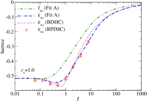
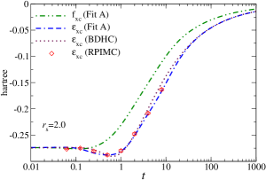
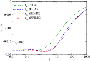
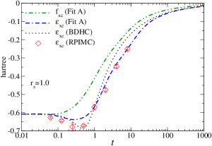
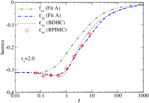
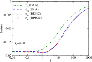
Figure 1: $\varepsilon_{\mathrm{xc}}$ and $f_{\mathrm{xc}}$ from Fit A for the unpolarized, $\zeta=0$ (top) and the fully polarized, $\zeta=1$ (bottom) HEG at $r_{s}=1$, 2 and 40 along with RPIMC data and BDHC fit for $\varepsilon_{\mathrm{xc}}$.

We now turn to intermediate polarizations. In principle the XC functional has separate exchange and correlation contributions. At $T=0$ K, exact spin scaling Oliver.Perdew.1979 defines the X functional for arbitrary polarization in terms of the unpolarized one. The argument can be extended straightforwardly to $T>0$ K; see the Supplemental Material SM . No corresponding exact result is known for interpolating the C contribution between $\zeta=0$ and $\zeta=1$, so approximate forms are used. Moreover, it is convenient computationally to use an XC functional rather than separate X and C contributions. We used such a form,

$$f_{\mathrm{xc}}(r_{\mathrm{s}},T,\zeta) =f_{\mathrm{xc}}^{0}(r_{\mathrm{s}},t)$$

$$+ \Big{[}f_{\mathrm{xc}}^{1}(r_{\mathrm{s}},2^{-2/3}t)-f_{\mathrm{xc}}^{0}(r_{\mathrm{s}},t)\Big{]}\phi(r_{\mathrm{s}},t,\zeta)\;,$$ (17)

with $\phi(r_{\mathrm{s}},t,\zeta)$ the polarization interpolation function and $t$ on the right hand side chosen systematically to be that of the unpolarized case, $t=T/T_{F}^{\zeta=0}$, as well as in Eqs. (19) - (20) below. At $T=0$ KDreizlerGrossBook

$$\phi(\zeta)=\frac{(1+\zeta)^{\alpha}+(1-\zeta)^{\alpha}-2}{2^{\alpha}-2}\,,$$ (18)

with $\alpha=4/3$. Perrot and Dharma-wardana PDW2000 developed a finite-$T$ generalization, $\phi(r_{\mathrm{s}},t,\zeta)$, by replacing the exponent $\alpha=4/3$ with a function, $\alpha(r_{\mathrm{s}},t)$, as follows:

$$\alpha(r_{\mathrm{s}},t) = 2-g(r_{\mathrm{s}})\exp\{-t\lambda(r_{\mathrm{s}},t)\}$$

$$g(r_{\mathrm{s}}) = \frac{g_{1}+g_{2}r_{\mathrm{s}}}{1+g_{3}r_{\mathrm{s}}}$$

$$\lambda(r_{\mathrm{s}},t) = \lambda_{1}+\lambda_{2}tr_{\mathrm{s}}^{1/2}\;.$$ (19)

Their parametrization used classical map hypernetted chain data for the HEG and proper behavior as $T\rightarrow 0$ K. We have reparametrized $\phi(r_{\mathrm{s}},t,\zeta)$ using the more recent $T=0$ K QMC data (which includes intermediate polarizations $\zeta=0.34$, 0.66) SND.2013 along with the CHNC data for intermediate $\zeta=0.6$ in Table IV of Ref. PDW2000, . (Observe that this is the only use of those CHNC data in this work.) The result is a modest improvement for $T=0$ K. The new parameter values are in Table 3. The value of $g_{1}$ is fixed from the condition that $\lim_{r_{\mathrm{s}}\rightarrow 0}\phi(r_{\mathrm{s}},t=0,\zeta)=\phi(\zeta)$. The revised $\phi(r_{\mathrm{s}},t,\zeta)$ depends weakly on $t$ for all $r_{\mathrm{s}}$ and $\zeta$.

Table 3: Parameters for the polarization interpolation function given in Eqs. (18) and (19).

	$\nu=1$	$\nu=2$	$\nu=3$
$g_{\nu}$	2/3	-0.0139261	0.183208
$\lambda_{\nu}$	1.064009	0.572565	-

Exact spin interpolation for finite-$T$ exchange yields the exchange free energy

$$f_{\mathrm{x}}(r_{\mathrm{s}},T,\zeta)=\tfrac{1}{2}\Big{[}(1+\zeta)^{4/3}f_{\mathrm{x}}^{0}(r_{\mathrm{s}},t_{\uparrow})+(1-\zeta)^{4/3}f_{\mathrm{x}}^{0}(r_{\mathrm{s}},t_{\downarrow})\Big{]}\,,$$ (20)

where $t_{\uparrow/\downarrow}\equiv t(2n_{\uparrow/\downarrow},T)=2k_{B}T/[3\pi^{2}(2n_{\uparrow/\downarrow})]^{2/3}$, and $n_{\uparrow/\downarrow}=(1\pm\zeta)n/2$. (Note that $f_{\mathrm{x}}^{\zeta}$ for $\zeta=0,1$ given by Eq. (15) also is given both analytically as a Fermi integral and tabulated in Ref. Brown.PRL, Supplementary Material as $E_{x,HF}$.) Thus the correlation free energy can be found from Eqs. (17) and (20) to be

$$f_{\mathrm{c}}(r_{\mathrm{s}},T,\zeta)=f_{\mathrm{xc}}(r_{\mathrm{s}},T,\zeta)-f_{\mathrm{x}}(r_{\mathrm{s}},T,\zeta)\,.$$ (21)

To test the $T\rightarrow 0$ K limit of our interpolation, we calculated the correlation energy per particle

$$\varepsilon_{\mathrm{c}}(r_{\mathrm{s}},\zeta)\equiv f_{\mathrm{c}}(r_{\mathrm{s}},0,\zeta)=f_{\mathrm{xc}}(r_{\mathrm{s}},0,\zeta)-f_{\mathrm{x}}(r_{\mathrm{s}},0,\zeta)\,,$$ (22)

where $f_{\mathrm{x}}(r_{\mathrm{s}},0,\zeta)\equiv\varepsilon_{\mathrm{x}}(r_{\mathrm{s}},\zeta)$ is the LSDA X energy per particle. Comparison with the Perdew-Zunger (PZ) LSDA PZ81 and QMC simulation data shows excellent agreement as a function of $\zeta$ for $r_{\mathrm{s}}=$ 0.25, 0.5, 1, 2, 3, 5, 10, and 20, with the maximum relative difference between Eq. (22) and the PZ correlation energy about 4% at $r_{\mathrm{s}}=0.25$ and 0.5. (Also see Supplemental Material SM .)

In sum, we have extracted the XC free energy for the finite-$T$ HEG from the RPIMC data, parametrized it in a form with exact asymptotic limits ($r_{s}\ll 1$, $t=0$, and $t\gg 1$) for both the spin unpolarized and fully polarized cases, and provided a $T$-dependent interpolation for intermediate polarizations. The result, Eqs. (9)-(14) and (17)-(19) and associated parameters, is a proper finite-$T$ extension of the widely used ground-state LSDA.

Acknowledgments: We thank Ethan Brown for helpful correspondence and for providing the erratum to Ref. Brown.fit, prior to publication and Paul Grabowski and Aurora Pribram-Jones for a useful remark. We thank the University of Florida Research Computing Group for computational resources and technical support. VVK, JD, and SBT were supported by U.S. Dept. of Energy grant DE-SC0002139. TS was supported by the Dept. of Energy Office of Fusion Energy Sciences (FES).

References

- [1] E.W. Brown, B.K. Clark, J.L. DuBois, and D.M. Ceperley, Phys. Rev. Lett. 110, 146405 (2013).
- [2] J.P. Perdew, and A. Zunger, Phys. Rev. B 23, 5048 (1981).
- [3] S.H. Vosko, L. Wilk, and M. Nusair, Can. J. Phys. 58, 1200 (1980).
- [4] D.M. Ceperley and B.J. Alder, Phys. Rev. Lett. 45, 566 (1980).
- [5] G.G. Spink, R.J. Needs, and N.D. Drummond, Phys. Rev. B 88, 085121 (2013).
- [6] N.D. Mermin, Phys. Rev. 137, A1441 (1965).
- [7] M.V. Stoitsov and I.Zh. Petkov, Annals Phys. 185, 121 (1988).
- [8] R.M. Dreizler in The Nuclear Equation of State, Part A, W. Greiner and H. Stöcker eds., NATO ASI B216 (Plenum, NY, 1989) 521.
- [9] B. Holst, R. Redmer, and M.P. Desjarlais, Phys. Rev. B 77, 184201 (2008).
- [10] F. Lambert, J. Clèrouin, and G. Zèrah, Phys. Rev. E 73, 016403 (2006).
- [11] M.P. Surh, T.W. Barbee III, and L.H. Yang, Phys. Rev. Lett. 86, 5958 (2001).
- [12] V.V. Karasiev, T. Sjostrom, and S.B. Trickey, Phys. Rev. E 86, 056704 (2012).
- [13] V.V. Karasiev, D. Chakraborty, O.A. Shukruto, and S.B. Trickey, Phys. Rev. B 88, 161108(R) (2013).
- [14] S.X. Hu, B. Militzer, V.N. Goncharov, and S. Skupsky, Phys. Rev. B 84, 224109 (2011).
- [15] T. Sjostrom, F.E. Harris, and S.B. Trickey, Phys. Rev. B 85, 045125 (2012)
- [16] R.A. Lippert, N.A. Modine, and A.F. Wright, J. Phys.: Condens. Matter 18, 4295 (2006).
- [17] M. Greiner, P. Carrier, and A. Görling, Phys. Rev. B 81, 155119 (2010).
- [18] T. Sjostrom and J. Dufty, Phys. Rev. B 88, 115123 (2013).
- [19] E.W. Brown, J.L. DuBois, M. Holzmann, and D.M. Ceperley, Phys. Rev. B 88, 081102(R) (2013); ibid. 88, 199901(E) (2013).
- [20] R.P. Feynman, N. Metropolis, and E. Teller, Phys. Rev. 75, 1561 (1949).
- [21] V.V. Karasiev, T. Sjostrom, and S.B. Trickey, Phys. Rev. B 86, 115101 (2012).
- [22] S. Tanaka, S. Mitake, and S. Ichimaru, Phys. Rev. A 32, 1896 (1985);
- [23] H.K. Schweng, and H.M. Böhm, Phys. Rev. B 48, 2037 (1993).
- [24] F. Perrot and M.W.C. Dharma-wardana, Phys. Rev. B 62, 16536 (2000); ibid. 67, 079901(E) (2003).
- [25] See Supplemental Material at http://link.aps.org/… for details.
- [26] S. Tanaka and S. Ichimaru, J. Phys. Soc. Jpn. 55, 2278 (1986).
- [27] S. Tanaka, and S. Ichimaru, Phys. Rev. B 39, 1036 (1989).
- [28] S. Ichimaru, Rev. Mod. Phys. 65, 255 (1993).
- [29] F. Perrot and M.W.C. Dharma-wardana, Phys. Rev. A 30, 2619 (1984).
- [30] F. Perrot, Phys. Rev. A 20, 586 (1979).
- [31] H.E. DeWitt, J. Math. Phys. 7, 616 (1965).
- [32] J.P. Perdew and Y. Wang, Phys. Rev. B 45, 13244 (1992).
- [33] G.L. Oliver, and J.P. Perdew, Phys. Rev. A 20, 397 (1979).
- [34] R.M. Dreizler and E.K.U. Gross, Density Functional Theory (Springer-Verlag, Berlin, 1990). See p. 178.