Performance measures for single-degree-of-freedom energy harvesters under stochastic excitation

Abstract

We develop performance criteria for the objective comparison of different classes of single-degree-of-freedom oscillators under stochastic excitation. For each family of oscillators, these objective criteria take into account the maximum possible energy harvested for a given response level, which is a quantity that is directly connected to the size of the harvesting configuration. We prove that the derived criteria are invariant with respect to magnitude or temporal rescaling of the input spectrum and they depend only on the relative distribution of energy across different harmonics of the excitation. We then compare three different classes of linear and nonlinear oscillators and using stochastic analysis methods we illustrate that in all cases of excitation spectra (monochromatic, broadband, white-noise) the optimal performance of all designs cannot exceed the performance of the linear design. Subsequently, we study the robustness of this optimal performance to small perturbations of the input spectrum and illustrate the advantages of nonlinear designs relative to linear ones.

1 Introduction

Energy harvesting is the process of targeted energy transfer from a given source (e.g. ambient mechanical vibrations, water waves, etc) to specific dynamical modes with the aim of transforming this energy to useful forms (e.g. electricity). In general, a source of mechanical energy can be described in terms of the displacement, velocity or acceleration spectrum. Moreover, in most cases the existence of the energy harvesting device does not alter the properties of the energy source i.e. the device is essentially driven by the energy source in a one-way interaction.

Typical energy sources are usually characterized by non-monochromatic energy content, i.e. the energy is spread over a finite band of frequencies. This feature has led to the development of various techniques in order to achieve efficient energy harvesting. Many of these approaches employ single-degree-of-freedom oscillators with non-quadratic potentials, i.e. with a restoring force that is nonlinear see e.g. [1, 2, 3, 4, 5, 6, 7, 8, 9, 10, 11, 12, 13]. In all of these approaches, a common characteristic is the employment of intensional nonlinearity in the harvester dynamics with an ultimate scope of increasing performance and robustness of the device without changing its size, mass or the amount of its kinetic energy. Even though for linear systems the response of the harvester can be fully characterized (and therefore optimized) in terms of the energy-source spectrum (see e.g. [4, 14]), this is not the case for nonlinear systems which are simultaneously excited by multiple harmonics - in this case there are no analytical methods to express the stochastic response in terms of the source spectrum. While in many cases (e.g. in [3, 6, 8, 13]) the authors observe clear indications that the energy harvesting capacity is increased in the presence of nonlinearity, in numerous other studies (e.g. [2, 1, 5, 7]) these benefits could not be observed. To this end it is not obvious if and when a class (i.e. a family) of nonlinear energy harvesters can perform “better” relative to another class (of linear or nonlinear systems) of energy harvesters when these are excited by a given source spectrum.

Here we seek to define objective criteria that will allow us to choose an optimal and robust energy harvester design for a given energy source spectrum. An efficient energy harvester (EH) can be informally defined as the configuration that is able to harvest the largest possible amount of energy for a given size and mass. This is a particularly challenging question since the performance of any given design depends strongly on the chosen system parameters (e.g. damping, stiffness, etc.) and in order to compare different classes of systems (e.g. linear versus nonlinear) the developed measures should not depend on the specific system parameters but rather on the form of the design, its size or mass as well as the energy source spectrum. Similar challenges araise when one tries to quantify the robustness of a given design to variations of the source spectrum for which it has been optimized.

To pursue this goal we first develop measures that quantify the performance of general nonlinear systems from broadband spectra, i.e. simultaneous excitation from a broad range of harmonics. These criteria demonstrate for each class of systems the maximum possible power that can be harvested from a fixed energy source using a given volume. We prove that the developed measures are invariant to linear transformations of the source spectrum (i.e. rescaling in time and size of the excitation) and they essentially depend only on its shape, i.e. the relative distribution of energy among different harmonics. For the sake of simplicity, we will present our measures for one dimensional systems although they can be generalized to higher dimensional cases in a straightforward manner.

Using the derived criteria we examine the relative advantages of different classes of single-degree-of-freedom (SDOF) harvesters. We examine various extreme scenarios of source spectra ranging from monochromatic excitations to white-noise cases (also including the intermediate case of the Pierson-Moskowitz (PM) spectrum). We prove that there are fundamental limitations on the maximum possible harvested power that can be achieved (using SDOF harvesters) and these are independent from the linear or nonlinear nature of the design. Moreover, we examine the robustness properties of various SDOF harvester designs when the source characteristics are perturbed and we illustrate the dynamical regimes where non-linear designs are preferable compared with the linear harvesters.

2 Quantification of power harvesting performance under broadband excitation

We study the energy harvesting properties of a SDOF oscillator subjected to random excitation. In the energy harvesting setting, randomness is usually introduced through the excitation signal which although is characterized by a given spectrum, i.e. a given amplitude for each harmonic, the relative phase between harmonics is unknown and to this end is modeled as a uniformly distributed random variable. We consider the following system consisting of an oscillator lying on a basis whose displacement $h\left(t\right)$ is a random function of time with given spectrum. The equation of motion for this simple system has the form

$$m\ddot{x}+\lambda\left(\dot{x}-\dot{h}\right)+F\left(x-h\right)=0,$$ (1)

where $m$ is the mass of the system, $\lambda$ is a dissipation coefficient expressing only the harvesting of energy (we ignore in this simple setting any mechanical loses), and $F$ is the spring force that has a given form but free parameters, i.e. $F\left(x\right)=F\left(x;k_{1},...,k_{n}\right).$ One could think of $F$ as a polynomial: $F\left(x;k_{p}\right)={\sum\limits_{p=1,...,N}}k_{p}x^{p}$.

We assume that the excitation process is stationary and ergodic having a given spectrum $S_{hh}\left(\omega\right)$ (See Appendix I for definition). We also assume that after sufficient time the system converges to a statistical steady state where the response can be characterized by the power spectrum $S_{qq}\left(\omega\right).$ For this system the harvested power per unit mass is given by

$$P_{h}=\frac{\lambda}{m}\overline{\left(\dot{x}-\dot{h}\right)^{2}},$$ (2)

where the bar denotes ensemble or temporal average in the statistical steady state regime of the dynamics. For convenience we apply the transformation $x-h=q$ to obtain the system

$$\ddot{q}+\hat{\lambda}\dot{q}+\hat{F}\left(q\right)=-\ddot{h},$$ (3)

where $\hat{\lambda}=\frac{\lambda}{m}$ and $\hat{F}=\frac{F}{m}.$

Through this formulation we note that the mass can be regarded as a parameter that does not need to be taken into account in the optimization procedure. This is because for any optimal set of parameters $\hat{\lambda}$ and $\hat{F}$, the energy harvested will increase linearly with the mass of the oscillator employed (given that $\hat{\lambda}$ and $\hat{F}$ remain constant).

2.1 Absolute and normalized harvested power $P_{h}$

In the present work, we are interested to compare the maximum possible performance between different classes of oscillators and to this end we ignore mechanical losses and assume that the damping coefficient $\hat{\lambda}$ describes entirely the energy harvested. In terms of the spectral properties of the response, the absolute harvested power $P_{h}$ can then be expressed as

$$P_{h}=\hat{\lambda}\overline{\dot{q}^{2}}=\hat{\lambda}{\displaystyle\int\limits_{-\infty}^{\infty}}\omega^{2}S_{qq}\left(\omega\right)d\omega.$$ (4)

This quantifies the amount of energy harvested per unit mass.

2.2 Size of the energy harvester $\mathcal{B}$

An objective comparison between two harvesters should involve not only the same mass but also the same size. We chose to quantify the characteristic size of the harvesting device using the mean square displacement of the center of mass of the system. For the SDOF setting, this is simply the typical deviation of the stochastic process $q\left(t\right)$ given by

$$d=\sqrt{\overline{q^{2}}}=\sqrt{{\displaystyle\int\limits_{-\infty}^{\infty}}S_{qq}\left(\omega\right)d\omega}.$$ (5)

Our goal is to quantify the maximum performance of a harvesting configuration for a given typical size $d$ and for a given form of input spectrum. To achieve invariance with respect to the source-spectrum magnitude, we will use the non-dimensional ratio

$$\mathcal{B}=\frac{\overline{q^{2}}}{\overline{h^{2}}},$$ (6)

which is the square of the relative magnitude of the device compared with the typical size of the excitation motion $\sqrt{\overline{h^{2}}}$. The above quantity also expresses the amount of energy that the device carries relative to the energy of the excitation and to this end we will refer to it as the response level of the harvester. It will be used to parametrize the performance measures developed in the next section with respect to the typical size of the device.

2.3 Harvested power density $\rho_{e}$

For each response level $\mathcal{B}$, we define the harvested power density $\rho_{e}$ as the maximum possible harvested power $\underset{\left\{\hat{\lambda},\hat{k}_{i}\text{ }|\text{ }\mathcal{B}\right\}}{\max}P_{h}$ (for a given excitation spectrum and under the constraint of a given response level $\mathcal{B}$) suitably normalized with respect to the response size $\overline{q^{2}}$ and the mean frequency of the input spectrum

$$\rho_{e}(\mathcal{B})=\frac{\underset{\left\{\hat{\lambda},\hat{k}_{i}\text{ }|\text{ }\mathcal{B}\right\}}{\max}P_{h}}{\omega_{h}^{3}\overline{q^{2}}}=\frac{\underset{\left\{\hat{\lambda},\hat{k}_{i}\text{ }|\text{ }\mathcal{B}\right\}}{\max}\left(\hat{\lambda}\overline{\dot{q}^{2}}\right)}{\omega_{h}^{3}\overline{q^{2}}}$$ (7)

where the mean frequency of the input spectrum is defined as

$$\omega_{h}=\frac{1}{\overline{h^{2}}}{\int\limits_{0}^{\infty}}\omega S_{hh}\left(\omega\right)d\omega.$$ (8)

This measure should be viewed as a function of the response level of the device $\mathcal{B}$. As we show below it satisfies an invariance property under linear transformations of the excitation spectrum, i.e. rescaling of the spectrum in time and magnitude (Figure 1). More specifically we have the following theorem.

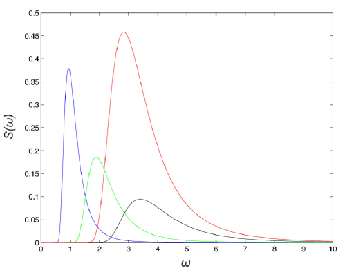
Figure 1: Various spectral curves obtained by magnitude and temporal rescaling of the Pierson-Moskowitz spectrum. Amplification and stretching of the input spectrum will leave the effective damping and the harvested power density invariant.

Theorem 1

The harvested power density $\rho_{e}$ is invariant with respect to linear transformations of the input energy spectrum $S_{hh}\left(\omega\right)$ (uniform amplification and stretching). In particular, under the modified excitation $g\left(t\right)=a\sqrt{b}h\left(bt\right)$ or equivalently the input spectrum $S_{gg}\left(\omega\right)=a^{2}S_{hh}\left(\frac{\omega}{b}\right)$, where $a>0$ and $b>0$ , the curve $\rho_{e}\left(\mathcal{B}\right)$ remain invariant.

Proof. Let $\hat{\lambda}_{0}$ and $\hat{k}_{i,0}$ be the optimal parameters for which the quantity $P_{h}$ attains its maximum value for the input spectrum $S_{hh}\left(\omega\right)$ under the constraint of a given response level $\mathcal{B}_{0}=\frac{\overline{q^{2}}}{\overline{h^{2}}}.$ For convenience, we will use the notation $\hat{F}_{0}\left(q\right)=\hat{F}\left(q;\hat{k}_{1,0},...,\hat{k}_{n,0}\right).$ For these optimal parameters we will also have the optimum response $q_{0}\left(t\right)$ that satisfies the equation

$$\ddot{q}_{0}+\hat{\lambda}_{0}\dot{q}_{0}+\hat{F}_{0}\left(q_{0}\right)=-\ddot{h}.$$ (9)

We will prove that under the rescaled spectrum $S_{gg}\left(\omega\right)=a^{2}S_{hh}\left(\frac{\omega}{b}\right)$ the harvested power density curve $\rho_{e}\left(\mathcal{B}\right)$ remains invariant. By direct computation, it can be verified that the modified spectrum $S_{gg}\left(\omega\right)$ corresponds to an excitation of the form

$$g\left(t\right)=a\sqrt{b}h\left(bt\right).$$ (10)

Moreover, by direct calculation we can verify that

$$\overline{g^{2}}=a^{2}b\overline{h^{2}}\text{ \ \ \ and \ \ \ }\omega_{g}=b\omega_{h}.$$ (11)

We pick a response level $\mathcal{B}_{0}$ for the system excited by $h\left(t\right)\$and we will prove that $\rho_{e,g}\left(\mathcal{B}_{0}\right)=\rho_{e,h}\left(\mathcal{B}_{0}\right).$ Under the new excitation the system equation will be

$$\ddot{q}+\hat{\lambda}\dot{q}+\hat{F}\left(q\right)=-a\sqrt{b}\frac{d^{2}h\left(bt\right)}{dt^{2}}.$$ (12)

We apply the temporal transformation $bt=\tau.$ In the new timescale, we will have (differentiation is now denoted with ^′)

$$b^{2}q^{\prime\prime}+\hat{\lambda}bq^{\prime}+\hat{F}\left(q\right)=-ab^{\frac{5}{2}}h^{\prime\prime}.$$ (13)

For $\frac{\overline{q^{2}}}{\overline{g^{2}}}=\mathcal{B}_{0}$, we want to find the set of parameters $\hat{\lambda}$ and $\hat{k}_{i}$ that will maximize $P_{g}=\hat{\lambda}\overline{\dot{q}^{2}}$ given the dynamical constraint (12). This optimized quantity can also be written as

$$P_{g}=\hat{\lambda}\overline{\dot{q}^{2}}=b^{2}\hat{\lambda}\overline{q^{\prime 2}},$$ (14)

where $q^{\prime}$ is described by the rescaled equation (13). However, the optimization problem in equations (13) and (14) is identical with the original one given by equation (9) and it has an optimal solution when $\hat{\lambda}=b\hat{\lambda}_{0}$ and $\hat{F}\left(q\right)=ab^{\frac{5}{2}}\hat{F}_{0}\left(\frac{q}{a\sqrt{b}}\right).$ For this set of parameters, equation (13) coincides with equation (9) and the solution to (13) will be $q\left(t\right)=a\sqrt{b}q_{0}\left(bt\right)$. Note that for this solution we also have

$$\frac{\overline{q^{2}}}{\overline{g^{2}}}=\frac{a^{2}b\overline{q_{0}^{2}}}{a^{2}b\overline{h^{2}}}=\frac{\overline{q_{0}^{2}}}{\overline{h^{2}}}=\mathcal{B}_{0},$$ (15)

and therefore the optimized solution that we found corresponds to the correct response level. The last step is to compute the harvested power density for the new solution. These will be given by

$$\rho_{e,g}({\mathcal{B}_{0}})=\frac{\underset{\left\{\hat{\lambda},\hat{k}_{i}\text{ }|\text{ }\mathcal{B}_{0}\right\}}{\max}\left(\hat{\lambda}\overline{\dot{q}^{2}}\right)}{\omega_{g}^{3}\overline{q^{2}}}=\frac{\underset{\left\{\hat{\lambda},\hat{k}_{i}\text{ }|\text{ }\mathcal{B}_{0}\right\}}{\max}\left(b^{2}\hat{\lambda}\overline{q^{\prime 2}}\right)}{\left(b^{3}\omega_{h}^{3}\right)\left(a^{2}b\overline{q_{0}^{2}}\right)}=\frac{\left(b\hat{\lambda}_{0}\right)\left(b^{3}a^{2}\overline{q_{0}^{\prime 2}}\right)}{\left(b^{3}\omega_{h}^{3}\right)\left(a^{2}b\overline{q_{0}^{2}}\right)}=\frac{\hat{\lambda}_{0}\overline{q_{0}^{\prime 2}}}{\omega_{h}^{3}\overline{q_{0}^{2}}}=\rho_{e,h}({\mathcal{B}_{0}}).$$ (16)

This completes the proof.

We emphasize that the above property can be generalized for multi-dimensional systems; a detailed study for this case will be presented elsewhere. Through this result we have illustrated that both uniform amplification and stretching of the input spectrum (see e.g. Figure 1 various amplified, and stretched versions of the Pierson-Moskowitz) will leave the harvested power density unchanged, and therefore the shape of spectrum is the only factor (i.e. relative distribution of energy between harmonics) that modifies the harvested power density.

Another important property of the developed measure is its independence of the specific values of the system parameters since it always refers to the optimal configuration for each design. Thus, it is an approach that characterizes a whole class of systems rather than specific members of this class. To this end it is suitable for the comparison of systems having different forms e.g. having different function $\hat{F}\left(q;\hat{k}_{1},...,\hat{k}_{n}\right)$ since it is only the form of the system that is taken into account and not the specific parameters $\hat{\lambda}$ and $\hat{k}_{1},...,\hat{k}_{n}$.

These two properties give an objective character to the derived measure as it depends only on the form of the employed configuration and the form of the input spectrum. For this reason, it can be used to perform systematic comparisons and optimizations among different classes of system configurations, e.g. linear versus nonlinear harvesters. In addition to the above properties, the curve $\rho_{e}\left(\mathcal{B}\right)$ reveals the optimal response level $\overline{q^{2}}$ so that the harvested power over the response magnitude is maximum, achieving in this way optimal utilization of the device size.

We note that for a multi-dimensional energy harvester it may also be useful to quantify the harvester performance using the effective harvesting coefficient $\lambda_{e}$ which is defined as the maximum possible harvested power $\underset{\left\{\hat{\lambda},\hat{k}_{i}\text{ }|\text{ }\mathcal{B}\right\}}{\max}P_{h}$ (for a given excitation spectrum and under the constraint of a given response level $\mathcal{B}$) normalized by the total kinetic energy of the device $E_{K}:$

$$\lambda_{e}(\mathcal{B})=\frac{\underset{\left\{\hat{\lambda},\hat{k}_{i}\text{ }|\text{ }\mathcal{B}\right\}}{\max}P_{h}}{\omega_{h}E_{K}},$$ (17)

where we have also non-dimensionalized with the mean frequency of the input spectrum so that the ratio satisfies similar invariant properties under linear transformations of the input spectrum. Although for MDOF systems the above measure can provide useful information about the efficient utilization of kinetic energy, for SDOF systems of the form (1) we always have $\lambda_{e}(\mathcal{B})=\hat{\lambda}$ and to this end we will not study this measure further in this work.

3 Quantification of performance for SDOF harvesters

We now apply the derived criteria in order to compare three different classes of nonlinear SDOF energy harvesters excited by three qualitatively different source spectra. In particular, we compare the performance of linear SDOF harvesters with two classes of nonlinear oscillators: an essentially nonlinear with cubic nonlinearity (mono-stable system) and one that has also cubic nonlinearity but negative linear stiffness (double well potential system or bistable) as illustrated in Figure 2. The first family of systems has been studied in various contexts with main focus the improvement of the energy harvesting performance from wide-band sources. The second family of nonlinear oscillators is well known for its property to maintain constant vibration amplitudes even for very small excitation levels, and it has also been applied to enhance the energy harvesting capabilities of nonlinear energy harvesters. More specifically we consider the following three classes of systems (Figure 3):

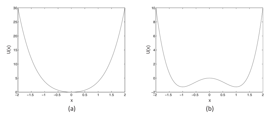
Figure 2: The shapes of potential function $U(x)=\frac{1}{2}\hat{k}_{1}x^{2}+\frac{1}{4}\hat{k}_{3}x^{4}$. (a) The monostable potential function with $\hat{k}_{1}>0$ and $\hat{k}_{3}>0$. (b) The bistable potential function with $\hat{k}_{1}<0$ and $\hat{k}_{3}>0$.

$$\ddot{q}+\hat{\lambda}\dot{q}+\hat{k}_{1}q =-\ddot{h},\text{ \ \ \ \ \ \ \ \ \ \ \ \ \ \ \ \ \ \ (linear system)}$$ (18)

$$\ddot{q}+\hat{\lambda}\dot{q}+\hat{k}_{3}q^{3} =-\ddot{h},\text{ \ \ \ \ \ \ \ \ \ \ \ \ \ \ \ \ \ \ (cubic system)}$$ (19)

$$\ddot{q}+\hat{\lambda}\dot{q}-\hat{\nu}q+\hat{k}_{3}q^{3} =-\ddot{h}.\text{ \ \ \ \ \ \ \ \ \ \ \ \ \ \ \ \ \ \ (negative stiffness)}$$ (20)

Our comparisons are presented for three cases of excitation spectra, namely: the monochromatic excitation, the white noise excitation, and an intermediate one characterized by colored noise excitation with Gaussian, stationary probabilistic structure and a power spectrum having the Pierson-Moskowitz form

$$S_{hh}=\frac{1}{\omega^{5}}\exp\left(-\omega^{-4}\right).$$ (21)

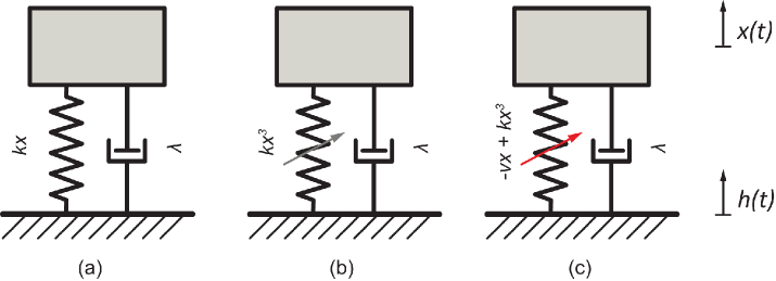
Figure 3: Linear and nonlinear SDOF systems: (a) Linear SDOF system, (b) Nonlinear SDOF system only with a cubic spring, and (c) Nonlinear SDOF system with the combination of a negative linear and a cubic spring.

The monochromatic and the white noise excitations are characterized by diametrically opposed spectral properties: the first case is the extreme form of a narrow-band excitation, while the second represents the most extreme case of a wide-band excitation. Our goal is to understand and objectively compare various designs that have been employed in the past to achieve better performance from sources which are either monochromatic or broad-band. We are also interested to use these two prototype forms of excitation in order to interpret the behavior of SDOF harvesters for intermediate cases of excitation such as the PM spectrum.

We first present the monochromatic and the white noise cases where many of the results can be derived analytically. We analyze the critical differences in terms of the harvester performance and subsequently, we numerically perform stochastic optimization of the nonlinear designs for the intermediate PM spectrum. For the PM excitation, we employ a discrete approximation of the excitation $h$ in spectral space, with harmonics that have given amplitude but relative phase differences modeled as uniformly distributed random variables. The responses of the dynamical systems (18) and (19) are then characterized by averaging (after sufficient time so that transient effects do not contribute) over a large ensemble of realizations, i.e. averaging over a large number of excitations $h$ generated with a given spectrum but randomly generated phases.

3.1 SDOF harvester under monochromatic excitation

Linear system. We calculate the harvested power density $\rho_{e}$ for the the linear oscillator under monochromatic excitation, i.e. the one-sided power spectrum is given by $S_{hh}\left(\omega\right)=\alpha^{2}\delta\left(\omega-\omega_{0}\right)$. For this case the computation can be carried out analytically. In particular for the linear oscillator we will have the power spectrum for the response given by

$$S_{qq}\left(\omega\right)=\frac{\omega^{4}}{\left(\hat{k}_{1}-\omega^{2}\right)^{2}+\hat{\lambda}^{2}\omega^{2}}S_{hh}\left(\omega\right).$$ (22)

Thus, the response level can be computed as

$$\mathcal{B}=\frac{\overline{q^{2}}}{\overline{h^{2}}}=\frac{\omega_{0}^{4}}{\left(\hat{k}_{1}-\omega_{0}^{2}\right)^{2}+\hat{\lambda}^{2}\omega_{0}^{2}},$$ (23)

where $\overline{h^{2}}$ is simply $\alpha^{2}$. Moreover, the average rate of energy harvested per unit mass will be given by

$$P_{h}=\hat{\lambda}\overline{\dot{q}^{2}}=\hat{\lambda}\alpha^{2}\frac{\omega_{0}^{6}}{\left(\hat{k}_{1}-\omega_{0}^{2}\right)^{2}+\hat{\lambda}^{2}\omega_{0}^{2}}.$$ (24)

Then we will have from equation (23)

$$\left(\hat{k}_{1}-\omega_{0}^{2}\right)^{2}+\hat{\lambda}^{2}\omega_{0}^{2}=\frac{\omega_{0}^{4}}{\mathcal{B}}.$$ (25)

Thus, for a given $\mathcal{B}$, the mean rate of energy harvested will be given by

$$P_{h}=\hat{\lambda}\overline{\dot{q}^{2}}=\hat{\lambda}\overline{q^{2}}\omega_{0}^{2}.$$ (26)

Therefore the mean rate of energy harvested will become maximum when $\hat{\lambda}$ is maximum. For fixed $\mathcal{B}$, equation (25) shows that the maximum legitimate value of $\hat{\lambda}$ will be given by $\hat{\lambda}=\frac{\omega_{0}}{\sqrt{\mathcal{B}}}$ and this can be achieved when $\hat{k}_{1}=\omega_{0}^{2}.$ Therefore we will have

$$P_{h} =\frac{\omega_{0}^{3}\overline{q^{2}}}{\sqrt{\mathcal{B}}}=\omega_{0}^{3}\overline{h^{2}}\sqrt{\mathcal{B}}=\alpha^{2}\omega_{0}^{3}\sqrt{\mathcal{B}},$$ (27)

$$\rho_{e} =\frac{\underset{\left\{\hat{\lambda},\hat{k}_{i}\text{ }|\text{{}}\mathcal{B}\right\}}{\max}P_{h}}{\omega_{h}^{3}\overline{q^{2}}}=\frac{1}{\sqrt{\mathcal{B}}}.$$ (28)

Hence, for a linear SDOF system under monochromatic excitation, the harvested power density is proportional to the magnitude of the square root of $\mathcal{B}$ while the harvested power is proportional to the square root of the response level.

Cubic and negative stiffness harvesters. For a nonlinear system the response under monochromatic excitation cannot be obtained analytically and to this end the computation will be carried out numerically. In figure 4, we present the response level $\mathcal{B}$ for all three systems (linear, cubic, and the one with negative stiffness with $\hat{\nu}=1$) for various system parameters. We also present the total harvested power superimposed with contours of the response level $\mathcal{B}$.

For both the linear and the cubic oscillator, we can observe the 1:1 resonance regime (see plots for the response level $\mathcal{B}$). For these two cases, we also observe a similar decay of the response level with respect to the damping coefficient. This behavior changes drastically in the negative stiffness oscillator where the response level is maintained with respect to changes of the damping coefficient. This is expected if one considers the double well form of the corresponding potential that controls the amplitude of the nonlinear oscillation. Despite the robust amplitude of the response, the performance (i.e. the amount of power being harvested) drops similarly with the other two oscillators (especially the cubic one) as the damping coefficient increases. Therefore robust response level does not necessarily imply constant performance level.

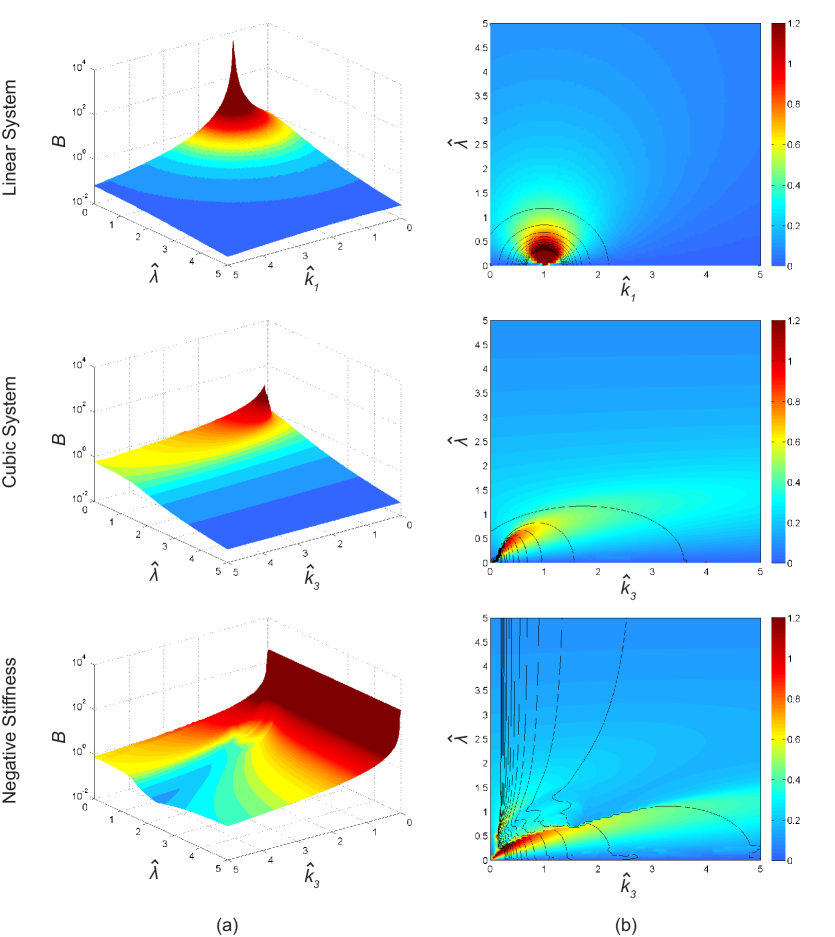
Figure 4: Response level $\mathcal{B}$ and power harvested for the case of monochromatic spectrum excitation over different system parameters. The response level $\mathcal{B}$ is also presented as a contour plot in the power harvested plots. All three cases of systems are shown: linear (top row), cubic (second row), and negative stiffness with $\hat{\nu}=1.$

To quantify the performance, we present in Figure 5 the maximum harvested power and the harvested power density for the three different oscillators. We observe that in all cases the linear design has superior performance compared with the nonlinear configurations. In addition, we note that the cubic and the negative stiffness oscillators have strongly variable performance which presents non-monotonic behavior with respect to the response level $\mathcal{B}$.

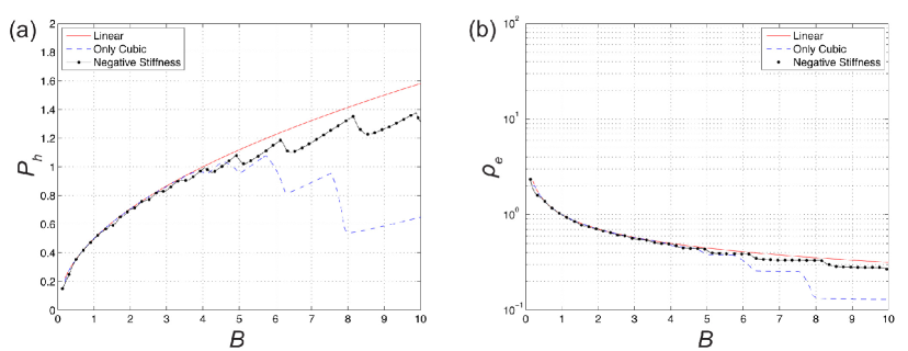
Figure 5: (a) Maximum harvested power, and (b) Power density for linear and nonlinear SDOF systems under monochromatic excitation.

To better understand the nature of this variability, we pick two characteristic values of $\mathcal{B}$ (one close to a local minimum i.e. $\mathcal{B=}8.5$ and one at a local maximum, i.e. $\mathcal{B=}8.1$) for the negative stiffness oscillator (Figure 5). From these points, we can observe that the strong performance for the nonlinear oscillator is associated with signatures of 1:3 resonance in the response spectrum. We also note that the small amplitude of the higher harmonic is not sufficiently large to justify the difference in the performance. On the other hand, the significant amplitude difference on the primary harmonic, which can be considered as an indirect effect of the 1:3 resonance, justifies the strong variability between the two cases.

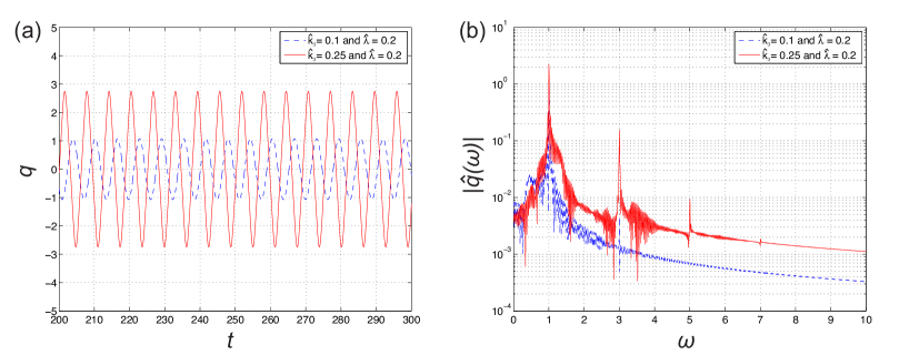
Figure 6: A nonlinear system with the combination of a negative linear ($\hat{\nu}=1$) and a cubic spring. Blue solid line corresponds to a local minimum of the performance in Fig. 4: $\hat{k}_{3}=0.1$ and $\hat{\lambda}=0.2$. Red dashed line corresponds to a local maximum of the performance in Fig. 4: $\hat{k}_{3}=0.25$ and $\hat{\lambda}=0.2$. (a) Response in terms of displacement. (b) Fourier transform modulus $\left|\hat{q}\left(\omega\right)\right|$.

Independently of the super-harmonic resonance occurring in the nonlinear designs for certain response levels, it is clear that the best performance for SDOF systems under monochromatic excitation can be achieved within the class of linear harvesters. To understand this result, we consider the general equation (3) multiplying with $\dot{q}$ and applying the mean value operator. This will give us the following energy equation

$$\frac{1}{2}\frac{d}{dt}\left(\overline{\dot{q}^{2}}\right)+\hat{\lambda}\overline{\dot{q}^{2}}+\overline{\hat{F}\left(q\right)\dot{q}}=-\overline{\ddot{h}\dot{q}}.$$ (29)

In a statistical steady state, we will have the first term vanishing. This is also the case for the third term, which represents the overall energy contribution from the conservative spring force. Moreover, the harvested power is equal to the second term and thus we have

$$P_{h}=\hat{\lambda}\overline{\dot{q}^{2}}=-\overline{\ddot{h}\dot{q}}.$$ (30)

For the monochromatic case, we have $\ddot{h}\left(t\right)=-\alpha\omega_{0}^{2}\cos\omega_{0}t.$ We represent the arbitrary statistical steady state response as

$$q={\displaystyle\sum\limits_{i}}\hat{q}_{i}\cos\left(\omega_{i}t+\phi_{i}\right),$$ (31)

with $\hat{q}_{i}>0$, and $\phi_{i}$ are phases determined from the system dynamics. From this representation, we obtain

$$P_{h}={\displaystyle\sum\limits_{i}}\hat{q}_{i}\alpha\omega_{0}^{2}\omega_{i}\lim_{T\rightarrow\infty}\frac{1}{T}{\displaystyle\int\limits_{0}^{T}}\cos\omega_{0}t\sin\left(\omega_{i}t+\phi_{i}\right)dt.$$ (32)

The quantity inside the integral will be nonzero only when $i=0$. Thus,

$$P_{h}=\hat{q}_{0}\alpha\omega_{0}^{3}\frac{\omega_{0}}{2\pi}{\displaystyle\int\limits_{0}^{\frac{2\pi}{\omega_{0}}}}\cos\omega_{0}t\sin\left(\omega_{0}t+\phi_{0}\right)dt=\frac{1}{2}\hat{q}_{0}\alpha\omega_{0}^{3}\sin\phi_{0}.$$ (33)

Note that from the representation for $q$, we obtain

$$\overline{q^{2}} ={\displaystyle\sum\limits_{i,j}}\hat{q}_{i}\hat{q}_{j}\overline{\cos\left(\omega_{i}t+\phi_{i}\right)\cos\left(\omega_{j}t+\phi_{j}\right)}$$

$$=\sum_{i,j(i\neq j)}\frac{1}{2}\hat{q}_{i}\hat{q}_{j}\overline{\{\cos([\omega_{i}-\omega_{j}]t+\phi_{i}-\phi_{j})+\cos([\omega_{i}+\omega_{j}]t+\phi_{i}+\phi_{j})\}}$$

$$\ \ +\sum_{i}\frac{1}{2}\hat{q}_{i}^{2}\overline{\{1+\cos(2\omega_{i}t+2\phi_{i})\}}$$

$$=\frac{1}{2}{\displaystyle\sum\limits_{i}}\hat{q}_{i}^{2}.$$ (34)

It is straightforward to conclude that for constant response level $\overline{q^{2}}$ the harvested power will become maximum when $\hat{q}_{0}$ is maximum, and this is the case only when all the energy of the response is concentrated in the harmonic $\omega_{0}$, a property that is guaranteed to occur for the linear systems. Thus, for SDOF harvesters, excited by monochromatic sources, the optimal linear system can be considered as an upper bound of the performance among the class of both linear and nonlinear oscillators.

3.2 SDOF harvester under white noise excitation

We investigated the monochromatic excitation case of both linear and nonlinear systems as an extreme case of a narrow-band excitation. The opposite extreme, the one that corresponds to a broadband excitation, is the Gaussian white noise. We consider a dynamical system governed by a second order differential equation under the standard Gaussian white noise excitation $\dot{W}(t)$ with zero mean and intensity equal to one (i.e. $\overline{W^{2}}=1$).

$$\ddot{q}+\hat{\lambda}\dot{q}+\hat{F}(q)=\alpha\dot{W}(t).$$ (35)

For this SDOF system, the probability density function is fully described by the Fokker-Planck-Kolmogorov equation which for the statistical steady state can be solved analytically providing us with the exact statistical response of system (35) in terms of the steady state probability density function (see e.g. [15])

$$p_{st}\left(q,\dot{q}\right)=C\exp\left({-\frac{\hat{\lambda}}{\alpha^{2}}\left[\frac{\dot{q}^{2}}{2}+\int_{0}^{q}\hat{F}(x)dx\right]}\right),$$ (36)

where $C$ is the normalization constant so that ${\displaystyle\iint}p_{st}\left(q,\dot{q}\right)dqd\dot{q}=1.$

In order to use previously developed measures, we define $\overline{h^{2}}=\alpha^{2}$ (the typical amplitude of the excitation is equal to the intensity of the noise). Moreover, since there is no characteristic frequency we can choose without loss of generality $\omega_{h}^{2}=1.$ Using expression (36), we can compute an exact expression for the harvested power

$$P_{\dot{W}}=\hat{\lambda}\overline{\dot{q}^{2}}=\alpha^{2}.$$ (37)

which is an independent quantity of the system parameters - the above result can be generalized in MDOF system as shown in [16]. We observe that in this extreme form of broadband excitation the harvested power is independent on the system parameters and depends only on the excitation energy level $\alpha.$ In addition, the harvested power density $\rho_{e}$ will be given by

$$\rho_{e}(\mathcal{B})=\frac{\underset{\left\{\hat{\lambda},\hat{k}_{i}\text{ }|\text{ }\mathcal{B}\right\}}{\max}P_{h}}{\omega_{h}^{3}\overline{q^{2}}}=\frac{\alpha^{2}}{\overline{q^{2}}}=\frac{1}{\frac{\overline{q^{2}}}{\overline{h^{2}}}}=\frac{1}{\mathcal{B}}.$$ (38)

Similarly with the harvested power, we observe that the harvested power density is also independent of the employed system design (Figure 7). Moreover, when we compare with the monochromatic excitation case (where we illustrated that the best possible performance can be achieved with linear systems), we see that the harvested power density drops faster with respect to the device size $\mathcal{B}$ when the energy is spread (in the spectral sense) compared with the case where energy is localized in a single input frequency.

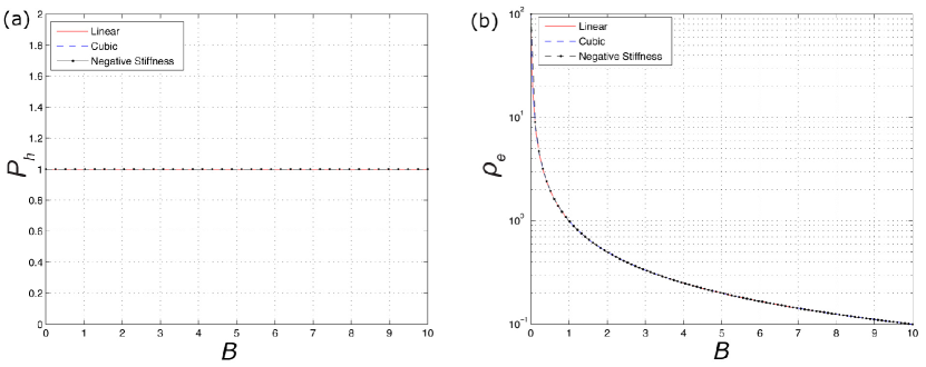
Figure 7: (a) Maximum harvested power, and (b) Power denstity for linear and nonlinear SDOF systems under white noise excitation.

3.3 SDOF harvester under colored noise excitation

The third case of our analysis involves a colored noise excitation, the Pierson-Moskowitz form (equation 21), which can be considered as an intermediate case between the two extremes presented previously. For a general excitation spectrum, the computation of the performance measures for the nonlinear systems has to be carried out numerically. However for the linear system the computation of the mean square amplitude and the mean rate of energy harvested per unit mass can be computed analytically [15]

$$\overline{q^{2}}\left(\hat{k}_{1},\hat{\lambda}\right) ={\displaystyle\int\limits_{0}^{\infty}}\frac{\omega^{4}}{\left(\hat{k}_{1}-\omega^{2}\right)^{2}+\hat{\lambda}^{2}\omega^{2}}\frac{1}{\omega^{5}}\exp\left(-\omega^{-4}\right)d\omega,$$ (39)

$$P_{h}\left(\hat{k}_{1},\hat{\lambda}\right) =\hat{\lambda}{\displaystyle\int\limits_{0}^{\infty}}\frac{\omega^{6}}{\left(\hat{k}_{1}-\omega^{2}\right)^{2}+\hat{\lambda}^{2}\omega^{2}}\frac{1}{\omega^{5}}\exp\left(-\omega^{-4}\right)d\omega.$$ (40)

For the nonlinear systems, we employ a Monte-Carlo method since the computational cost for simulating the SDOF harvester is reasonable. In particular, we generate random realizations which are consistent with the PM spectrum using a frequency domain method [17]. Subsequently, we simulate the dynamics of the SDOF long enough so that the system reaches a statistical steady state. The results are presented in Figure 8. We can still observe similar features with the monochromatic excitation even though the variations of response level and performance are now much smoother (compared with the monochromatic case). For the linear system, we do not have the sharp resonance peak that we had in the monochromatic case while the two nonlinear designs behave very similarly in terms of their performance maps. However, the characteristic difference of the negative stiffness design, related to the persistence of the response level even for large values of damping, is preserved in this non-monochromatic excitation case. Note that similarly to the monochromatic case this robustness in the response level does not necessarily imply strong harvesting power.

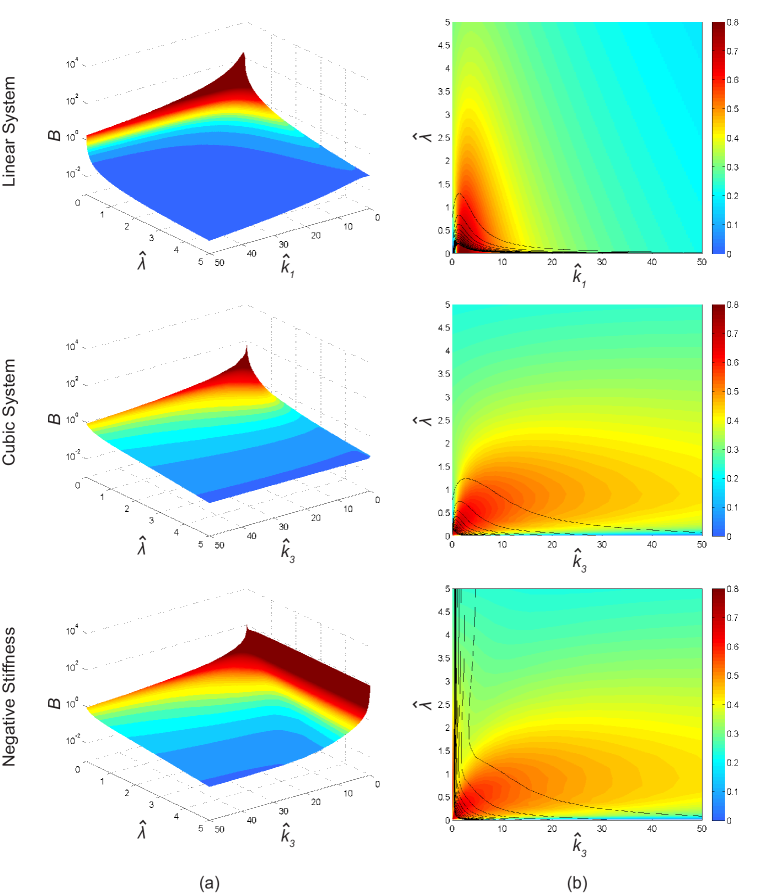
Figure 8: Response level $\mathcal{B}$ and power harvested for the case of excitation with Pierson-Moskowitz spectrum over different system parameters. The response level $\mathcal{B}$ is also presented as a contour plot in the power harvested plots. All three cases of systems are shown: linear (top row), cubic (second row), and negative stiffness with $\hat{\nu}=1.$

3.4 Comparison of the three different systems

A comparison of the linear system and the nonlinear systems under the Pierson-Moskowitz spectrum excitation is shown in Figure 9. As it can be seen from Figure 9b, the linear oscillator has the best performance compared to two nonlinear designs (note that for the negative stiffness oscillator a wide range of values $\hat{\nu}$ was employed and in all cases the results for the power density were qualitatively the same - to this end only the case $\hat{\nu}=1$ is presented). This is expected for any colored noise excitation, given that for the monochromatic extreme we have shown rigorously that the optimal performance of any nonlinear oscillator cannot exceed the optimal linear design, while for the white noise excitation all designs have identical performance. The relative performance in terms of harvested power for the three different classes of oscillators under three different types of excitations are summarized in Table 1.

Table 1: Harvested power of three different classes of oscillators under three different types of excitations. $\mathcal{L}$ denotes the linear oscillator, $\mathcal{M_{N}}$ denotes the monostable nonlinear oscillator, and $\mathcal{B_{N}}$ denotes the bistable nonlinear oscillator.

Excitation	Performance comparison
Monochromatic excitation	$\mathcal{L}>>\mathcal{B_{N}}>\mathcal{M_{N}}$
Colored noise excitation	$\mathcal{L}>\mathcal{M_{N}}>\mathcal{B_{N}}$
White noise excitation	$\mathcal{L}=\mathcal{M_{N}}=\mathcal{B_{N}}$

An important qualitative difference between the response under the Pierson-Moskowitz spectrum and the monochromatic excitation is the behavior of the harvested power for larger values of $\mathcal{B}$. While for the monochromatic case the harvested power scales with $\sqrt{\mathcal{B}}$, this is not the case for the colored noise excitation where the harvested power seems to converge to a finite value (a behavior that is consistent with the white noise excitation). Therefore, we can conclude that for small values of response level $\mathcal{B}$ the optimal performance under colored noise excitation behaves similarly with the monochromatic excitation while for larger values of $\mathcal{B}$ the optimal performance seems to be closer to the white-noise response. The above conclusions are also verified from Figure 10 where the three optimal harvested power density curves (corresponding to the three forms of excitation) are presented together. The performance of the optimal SDOF energy harvesters with respect to the size of the device $\mathcal{B}$ is incorporated in Table 2.

Table 2: The performance of optimal SDOF energy harvesters with respect to the size of the device. The number of $+$ indicates under which excitation the energy harvester performs relatively better.

Case	Monochromatic	Colored noise	White noise
$\mathcal{B}<1$	$+$	$++$	$+++$
$\mathcal{B}>1$	$+++$	$++$	$+$
$\mathcal{B}=1$	$+$	$+++$	$+$

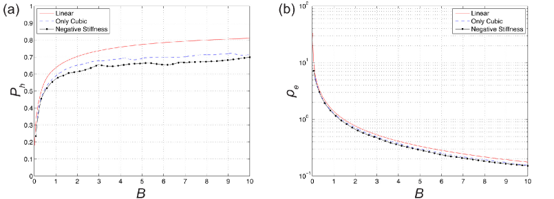
Figure 9: (a) Maximum harvested power, and (b) Power density for linear and nonlinear SDOF systems under Pierson-Moskowitz spectrum.

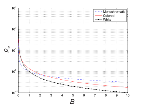
Figure 10: Harvested power density $\rho_{e}$ for the three different types of excitation spectra. The linear design is used in all cases since this is the optimal.

4 Quantification of performance robustness

We have examined the optimal performance for different designs of SDOF harvesters under various forms of random excitations. Even though the linear design has the optimal performance for fixed response level $\mathcal{B}$, the robustness of this performance under perturbations of the input spectrum characteristics (and with fixed optimal system parameters) has not been considered. This is the scope of this section where we investigate how linear and nonlinear systems with optimal system parameters behave when the excitation spectrum is perturbed.

More specifically, we are interested to investigate robustness properties with respect to frequency shifts of the excitation spectrum. Clearly, the harvested power and the response level (that characterizes the size of the device) will be affected by the spectrum shift. To quantify these variations we consider the following three ratios

$$\delta=\frac{B_{shifted}}{B_{0}},\text{ \ \ \ \ }\tau=\frac{(P_{h})_{shifted}}{(P_{h})_{0}},\text{\ \ \ \ \ \ }\sigma=\frac{(\rho_{e})_{shifted}}{(\rho_{e})_{0}},$$ (41)

where $\delta$ quantifies the variation of the response level ${\mathcal{B}}_{0}$ which essentially expresses the size of the device, $\tau$ quantifies exclusively the changes in performance while $\sigma$ shows the changes in harvested power density, i.e. it also takes into account the variations of the response level ${\mathcal{B}}$.

Monochromatic excitation. For the monochromatic excitation, perturbation in terms of spectrum shift can be expressed as

$$S_{hh}(\omega-\epsilon)=\delta(\omega-\omega_{0}-\epsilon).$$ (42)

where $\omega_{0}=1$. In Figure 11, we present the ratios describing the variation of the response level $\delta$, the harvested power $\tau$ and the harvested power density $\sigma$ in terms of perturbation $\epsilon$ for various levels of the unperturbed response level ${\mathcal{B}}$. For small response levels, i.e. when the system response is smaller than the excitation (${\mathcal{B=}}0.5$) we observe that the negative stiffness oscillator has more robustness to maintaining its response level when it is excited by lower frequencies $\left(\epsilon<0\right)$. For the same case, the harvested power decays in a similar fashion with the other two oscillators. Therefore, for $\epsilon<0$ and ${\mathcal{B=}}0.5$ the nonlinear oscillator with negative stiffness has the most robust performance. For faster excitations $\left(\epsilon>0\right)$ we observe that all oscillators drop their response level in smaller values than the design response level ${\mathcal{B}}_{0}$ with the linear system having the most robust behavior in terms of the total harvested power. We emphasize that as long as $\delta<1$ robustness is essentially defined by the largest value of $\tau$ among different types of oscillators.

For ${\mathcal{B=}}1$, we can observe that for all values of $\epsilon$ the negative stiffness oscillator has the most robust behavior in terms of the excitation level while the behavior of the harvested power is also better compared with the other two classes of oscillators. For larger values of the response level (${\mathcal{B=}}8$), we note that the response level ratio $\delta$ is maintained in levels below 1; therefore the size of the device will not be exceeded due to input spectrum shifts. On the other hand when we consider the variations of the harvested power, we observe that all in all the linear oscillators has the most robust behavior, while the two nonlinear oscillators drop suddenly their performance to very small levels for larger, positive values of $\epsilon.$

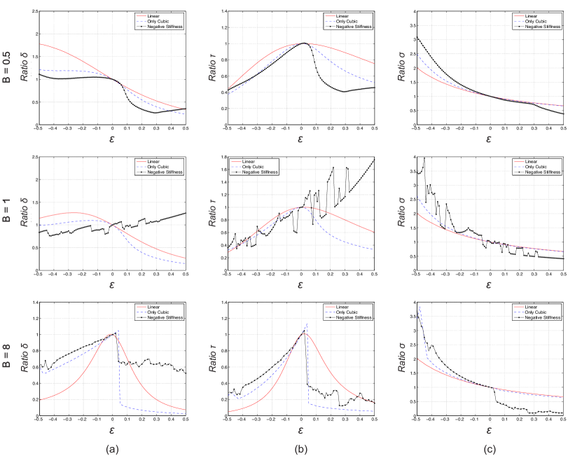
Figure 11: Robustness of (a) the response level, (b) the power harvested, and (c) the harvested power density for the monochromatic excitation under three regimes of operation: $\mathcal{B}=0.5$, $\mathcal{B}=1$, and $\mathcal{B}=8$.

Colored noise excitation. Similarly with the monochromatic case, we consider a small perturbation $\epsilon$ for the colored noise excitation spectrum:

$$S_{hh}(\omega-\epsilon)=\frac{1}{(\omega-\epsilon)^{5}}\exp\left(-(\omega-\epsilon)^{-4}\right).$$ (43)

The results are presented in Figure 12 for three different cases of unperturbed excitation levels ${\mathcal{B}}_{0}$. In contrast to the monochromatic case, the ratios $\delta,\tau,$ and $\sigma$ have much smoother dependence on the perturbation $\epsilon.$ Moreover, their variation is very similar for all three response levels ${\mathcal{B}}_{0}$. More specifically, we can clearly see that the two classes of nonlinear oscillators can better maintain their response level over all values of $\epsilon.$ On the other hand, the linear oscillator obtains a larger response level ${\mathcal{B}}$ when the spectrum is shifted to the right $\left(\epsilon>0\right)$ without substantially increasing the harvested power compared with the other two nonlinear oscillators. For $\epsilon<0$, all three families of oscillators harvest the same amount of energy. Thus, for colored noise excitation, the two families of nonlinear oscillators achieve the most robust performance. Hence, as long as the nonlinear design is chosen so that it has comparable optimal performance with the family of linear oscillators, it is the preferable choice since it has the best robustness properties.

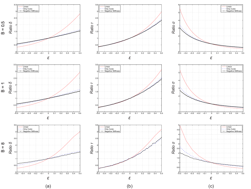
Figure 12: Robustness of (a) the response level, (b) the power harvested, and (c) the harvested power density for the PM spectrum excitation under three regimes of operation: $\mathcal{B}=0.5$, $\mathcal{B}=1$, and $\mathcal{B}=8$.

5 Conclusions

We have considered the problem of energy harvesting using SDOF oscillators. We first developed objective measures that quantify the performance of general nonlinear systems from broadband spectra, i.e. simultaneous excitation from a broad range of harmonics. These measures explicitly take into account the required size of the device in order to achieve this performance. We demonstrated that these measures do not depend on the magnitude or the temporal scale of the input spectrum but only the relative distribution of energy among different harmonics. In addition they are suitable to compare whole classes of oscillators since they always pick the most effective parameter configuration.

Using analytical and numerical methods, we applied the developed measures to quantify the performance of three different families of oscillators (linear, essentially cubic, and negative stiffness or bistable) for three different types of excitation spectra: an extreme form of a narrow band excitation (monochromatic excitation), an extreme form of a wide-band excitation (white-noise), and an intermediate case involving colored noise (Pierson-Moskowitz spectrum). For all three cases, we presented numerical and analytical arguments that the nonlinear oscillators can achieve in the best case equal performance with the optimal linear oscillator, given that the size of the device does not change. We also considered the robustness of each design to input spectrum shifts concluding that the nonlinear oscillator has the best behavior for the colored noise excitation. To this end, we concluded that, under a situation of designing a harvester with specific power, a nonlinear oscillator designed to achieve a performance that is close to the optimal performance of a linear oscillator is the best choice since it also has robustness against small perturbations.

Future work involves the generalization of the presented criteria to MDOF oscillators and the study of the benefits due to nonlinear energy transfers between modes [18, 19, 20, 21]. Preliminary results indicate that the application of nonlinear energy transfer ideas can have a significant impact on achieving higher harvested power density by distributing energy to more than one modes achieving in this way smaller required device size without reducing its performance level.

Acknowledgments. The authors would like to acknowledge the support from Kwanjeong Educational Foundation as well as a startup grant at MIT. TPS is also grateful to the American Bureau of Shipping for support under a Career Development Chair.

Appendix I: An overview of spectral properties for stationary and ergodic signals

Here we recall some basic properties for random signals. Let $h\left(t\right)$ be a stationary and ergodic signal for which we assume that it has finite power, i.e.

$$\lim_{T\rightarrow\infty}\frac{1}{2T}{\displaystyle\int\limits_{-T}^{T}}\left|h\left(t\right)\right|^{2}dt<\infty.$$

We define the correlation function

$$R_{hh}\left(\tau\right)=\lim_{T\rightarrow\infty}\frac{1}{2T}{\displaystyle\int\limits_{-T}^{T}}h\left(t\right)h\left(t+\tau\right)dt=\overline{h\left(t\right)h\left(t+\tau\right)},$$

where the bar denotes ensemble averaging and the last equality follows from the assumption of ergodicity. Note that we always have the property

$$\left|R_{hh}\left(\tau\right)\right|\leq R_{hh}\left(0\right).$$

Based on the correlation function, we can compute the power spectrum

$$S_{hh}\left(\omega\right)=\mathcal{F}\left[R_{hh}\left(\tau\right)\right]=\lim_{T\rightarrow\infty}\frac{1}{2T}\left|{\displaystyle\int\limits_{-T}^{T}}h\left(t\right)e^{-i\omega t}dt\right|^{2},$$

where the Fourier transform is given by

$$\mathcal{F}\left[R_{hh}\left(\tau\right)\right]={\displaystyle\int\limits_{-\infty}^{\infty}}R_{hh}\left(\tau\right)e^{-i\omega\tau}d\tau.$$

The power spectrum describes how the energy of a signal $h\left(t\right)$ is distributed among harmonics in an averaged sense. The total averaged energy of the signal is given by

$$E_{h}=\lim_{T\rightarrow\infty}\frac{1}{2T}{\displaystyle\int\limits_{-T}^{T}}\left|h\left(t\right)\right|^{2}dt=\overline{\left|h\left(t\right)\right|^{2}}=R_{hh}\left(0\right)=\frac{1}{2\pi}{\displaystyle\int\limits_{-\infty}^{\infty}}S_{hh}\left(\omega\right)d\omega.$$

In contrast to the usual energy spectrum defined by the magnitude of the Fourier transform of the signal, i.e. $S_{e}\left(\omega\right)=\left|\mathcal{F}\left[h\left(t\right)\right]\right|^{2},$ the power spectrum can be defined for a signal for which the energy ${\displaystyle\int\limits_{-T}^{T}}\left|h\left(t\right)\right|^{2}dt$ is not finite. Therefore we should see the power spectrum as a time or ensemble average of the energy distributed over different harmonics.

References

- [1] M. F. Daqaq, “Response of uni-modal duffing-type harvesters to random forced excitations,” Journal of Sound and Vibration, vol. 329, p. 3621, 2010.
- [2] M. F. Daqaq, “Transduction of a bistable inductive generator driven by white and exponentially correlated gaussian noise,” Journal of Sound and Vibration, vol. 330, no. 11, pp. 2554–2564, 2011.
- [3] P. Green, K. Worden, K. Atallah, and N. Sims, “The benefits of duffing-type nonlinearities and electrical optimisation of a mono-stable energy harvester under white gaussian excitations,” Journal of Sound and Vibration, vol. 331, no. 20, pp. 4504–4517, 2012.
- [4] N. Stephen, “On energy harvesting from ambient vibration,” Journal of Sound and Vibration, vol. 293, no. 1, pp. 409–425, 2006.
- [5] E. Halvorsen, “Fundamental issues in nonlinear wideband-vibration energy harvesting,” Physical Review E, vol. 87, no. 4, p. 042129, 2013.
- [6] D. A. Barton, S. G. Burrow, and L. R. Clare, “Energy harvesting from vibrations with a nonlinear oscillator,” Transactions of the ASME-L-Journal of Vibration and Acoustics, vol. 132, no. 2, p. 021009, 2010.
- [7] P. L. Green, E. Papatheou, and N. D. Sims, “Energy harvesting from human motion and bridge vibrations: An evaluation of current nonlinear energy harvesting solutions,” Journal of Intelligent Material Systems and Structures, 2013.
- [8] R. Harne and K. Wang, “A review of the recent research on vibration energy harvesting via bistable systems,” Smart Materials and Structures, vol. 22, no. 2, p. 023001, 2013.
- [9] V. Mendez, D. Campos, and W. Horsthemke, “Stationary energy probability density of oscillators driven by a random external force,” Physical Review E, vol. 87, p. 062132, 2013.
- [10] M. Brennan, B. Tang, G. P. Melo, and V. Lopes Jr, “An investigation into the simultaneous use of a resonator as an energy harvester and a vibration absorber,” Journal of Sound and Vibration, vol. 333, no. 5, 2014.
- [11] D. Watt and M. Cartmell, “An externally loaded parametric oscillator,” Journal of Sound and Vibration, vol. 170, no. 3, 1994.
- [12] C. McInnes, D. Gorman, and M. Cartmell, “Enhanced vibrational energy harvesting using nonlinear stochastic resonance,” Journal of Sound and Vibration, vol. 318, no. 4, 2008.
- [13] B. Mann and N. Sims, “Energy harvesting from the nonlinear oscillations of magnetic levitation,” Journal of Sound and Vibration, vol. 319, no. 1, 2009.
- [14] V. Méndez, D. Campos, and W. Horsthemke, “Efficiency of harvesting energy from colored noise by linear oscillators,” Physical Review E, vol. 88, no. 2, p. 022124, 2013.
- [15] K. Sobczyk, Stochastic Differential Equations. Dordrecht, The Netherlands: Kluwer Academic Publishers, 1991.
- [16] R. Langley, “A general mass law for broadband energy harvesting,” Journal of Sound and Vibration, In Press.
- [17] D. B. Percival, “Simulating gaussian random processes with specified spectra,” Computing Science and Statistics, vol. 24, pp. 534–538, 1992.
- [18] T. P. Sapsis, A. F. Vakakis, O. V. Gendelman, L. A. Bergman, G. Kerschen, and D. D. Quinn, “Efficiency of targeted energy transfer in coupled oscillators associated with 1:1 resonance captures: Part II, analytical study,” Journal of Sound and Vibration, vol. 325, pp. 297–320, 2009.
- [19] T. P. Sapsis, A. F. Vakakis, and L. A. Bergman, “Effect of stochasticity on targeted energy transfer from a linear medium to a strongly nonlinear attachment,” Probabilistic Engineering Mechanics, vol. 26, pp. 119–133, 2011.
- [20] T. P. Sapsis, D. D. Quinn, A. F. Vakakis, and L. A. Bergman, “Effective stiffening and damping enhancement of structures with strongly nonlinear local attachments,” ASME J. Vibration and Acoustics, vol. 134, p. 011016, 2012.
- [21] A. F. Vakakis, O. V. Gendelman, L. A. Bergman, D. M. McFarland, G. Kerschen, and Y. S. Lee, Nonlinear Targeted Energy Transfer in Mechanical and Structural Systems. Springer-Verlag, 2008.