Finite-frequency thermoelectric response in strongly correlated quantum dots

Abstract

We investigate the finite-frequency thermal transport through a quantum dot subject to strong interactions, by providing an exact, nonperturbative formalism that allows us to carry out a systematic analysis of the thermopower at any frequency. Special emphasis is put on the dc and high-frequency limits. We demonstrate that, in the Kondo regime, the ac thermopower is characterized by a universal function that we determine numerically.

I Introduction

In the quest to find the most energy-efficient systems and devices, thermal generation of currents in nanometer-size structures which can be manipulated by electric fields, may offer one of the best paths to follow. Sales et al. (1996); Snyder and Toberer (2008); Heremans et al. (2008) Quantum dots (QD) are among the best candidates, since they are highly tunable. Moreover, they are characterized by an enhanced figure of merit, as a result of the converging effect of reduced spatial dimensionality, that minimizes the phonon thermal conductivity, and an increased electronic density of states. So far, they can be used as thermoelectric power generators or coolers Humphrey et al. (2002), and when embedded into bulk materials or nanowires, a structure with large thermopower coefficient, $S$, is obtained. Harman et al. (2002); Wang et al. (2008) The same environment, however, is fundamentally enhancing the interaction between the electrons, generating strong correlations and other dynamical effects. By doing detailed measurements in QDs, it has been shown that the oscillating behavior of the thermopower as a function of the gate voltage might carry information on interactions present in the system.Svensson et al. (2012) On the theoretical side, the thermoelectric problem in quantum dots is also of considerable interest: First, a perturbative calculation valid for weakly interacting QDs was presented in Ref. Beenakker and Staring, 1992. Later on, in Refs. Boese and Fazio, 2001; Scheibner et al., 2005 the thermopower of a Kondo correlated dot was computed. Quite recently, by using the numerical renormalization group approach (NRG) approach, the thermoelectric properties of a strongly correlated dot modeled in terms of the Anderson model, were investigated systematically. Costi and Zlatić (2010) Other more exotic systems such as the SU(4) Kondo state Roura-Bas et al. (2012) or double-dot systemsTrocha and Barnaś (2012) were also studied, but, so far, mostly static effects have been addressed Donsa et al. (2013) and only few theoretical and experimental studies were focused on dynamical effects. Lim et al. (2013)

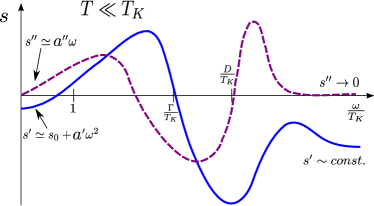
Figure 1: (Color online) Sketch of the real and imaginary parts of the universal function $s(\omega/T_{K},T/T_{K})$ in the Kondo regime, at a fixed temperature, $T\ll T_{K}$. The coefficients $a^{\prime}$ and $a^{\prime\prime}$ depend on temperature as $\sim 1/T^{2}$. See also Eq. (III) for the functional dependence of $s$.

In contrast, other transport quantities, such as the usual differential conductance or the noise, have been investigated at various frequencies. Sindel et al. (2005); Blanter and Sukhorukov (2000); Moca et al. (2011) Consequently, new interesting physics has emerged: It was found that the modulation of the gate voltages suppresses the Kondo temperature Kogan et al. (2004) $T_{K}$, and that the frequency-dependent emission noise of a quantum dot Basset et al. (2012) in the Kondo regime, at high frequencies, $\hbar\omega\gg k_{B}T_{K}$, provides information on the system at energy scales which are not accessible by simple dc measurements. Furthermore, in a slightly different context, i.e., the correlated band models, it has been predicted that the thermopower in the high-frequency limit may provide further understanding on the thermoelectric transport. Shastry (2006, 2009); Xu et al. (2011)

Motivated by these observations, we consider here the problem of thermoelectric response at finite frequencies in a quantum dot subject to a strong Coulomb interaction, and in particular we shall investigate the dynamical thermopower $S(\omega)$. This quantity characterizes how a charge current, $I^{(1)}(t)$, is generated by an infinitesimal time-dependent temperature difference $\delta T(t)$ across the dot and, at the same time, how a heat current $I^{(2)}(t)$ responds to an infinitesimal voltage drop $\delta V(t)$ Mah

$$\left(\begin{array}[]{c}\langle I^{(1)}(t)\rangle\\ \langle I^{(2)}(t)\rangle\end{array}\right) = \int dt^{\prime}dt^{\prime\prime}\,T\,S(t-t^{\prime})\,G(t^{\prime}-t^{\prime\prime})\times$$ (6)

$$\left(\begin{array}[]{c}\delta T(t^{\prime\prime})/T|_{\delta V=0}\\ \delta V(t^{\prime\prime})|_{\delta T=0}\end{array}\right)\,.$$

As defined, the thermopower itself is not a response function, so it can not be computed directly within the linear response theory. Instead, the combination $L_{12}(\omega)=TG(\omega)\,S(\omega)$ that appears in Eq. (6) is a true response function that can be computed exactly. To get the thermopower spectrum $S(\omega)$, aside from $L_{12}$ we also need the usual ac conductance, $G(\omega)=L_{11}(\omega)$. Then, $S(\omega)$ can be expressed as Shastry (2009); Luttinger (1964)

$$S(\omega)={1\over T}\left\{{L_{12}(\omega)\over L_{11}(\omega)}\right\}\,.$$ (7)

One of the main results of this work is that in the strong coupling (Kondo) regime, i.e., $\max\{\omega,T\}\ll T_{K}$, the equilibrium ac thermopower takes on a simple, universal form, which apart from a phase-dependent prefactor, is characterized by a universal function

$$S(\omega,T)\simeq{k_{B}\over e}\Big{(}{T\over T_{K}}\Big{)}\,s(\omega/T_{K},T/T_{K})\cot(\delta_{0})\,.$$ (8)

Here, $\delta_{0}$ is the phase shift of the electrons at the Fermi level, and the function $s$ is a complex universal function that depends exclusively on $\omega/T_{K}$ and $T/T_{K}$. The prefactor $k_{B}/e=8.6\times 10^{-5}\;V/K$ is the unit in which the thermopower is measured. The characteristic features of $s(\omega/T_{K},T/T_{K})$ are sketched in Fig. 1. At a given temperature $T\ll T_{K}$, and when $\omega\ll T_{K}$, the real part $s^{\prime}$ grows quadratically with the frequency $s^{\prime}\simeq s_{0}+a^{\prime}(T)\,\omega^{2}+\dots$, followed by multiple changes of sign at some intermediate frequencies, $\omega_{i}\sim\{T,\Gamma\}$, and becomes constant in the $\omega\to\infty$ limit. Its imaginary part vanishes in the $\omega\to 0$ limit, has a linear dependence $s^{\prime\prime}\simeq a^{\prime\prime}(T)\,\omega+\dots$ below the Kondo scale, and vanishes in the $\omega\to\infty$ limit.

In Fig. 2, we present a sketch of the setup. It consists of a quantum dot that is coupled to two external leads, $\alpha=\{L,R\}$, that have different temperatures, $T_{\alpha}(t)=T\pm\delta T(t)/2$. The temperature gradient $\delta T(t)$ generates a time-dependent current which flows across the dot. Starting from the Kubo formalism and Fourier transforming from time $t$ to frequency $\omega$, we find the ac thermopower, $S(\omega)$. We derive general, exact expressions for $L_{ij}(\omega)$, and implicitly for $S(\omega)$, which are valid at any frequency (see Eqs. (7) and (III)). The derivation is then followed by a careful analysis of different regimes of interest, such as the large-frequency limit, $S^{*}=S(\omega\to\infty)$, or the conventional low-frequency limit, $S_{0}=S(\omega=0)$ Costi and Zlatić (2010). As a technical observation, since we are interested in $S(\omega)$ at any frequency, even in the region $\omega\gg D$, the bandwidth $D$ of the conduction electrons must be kept finite in the calculations, otherwise an unphysical divergence with increasing frequency is present in the spectrum of $L_{12}(\omega)$ (see Sec. III).

The paper is organized as follows: In Sec. II, we introduce the model Hamiltonian and derive the exact expressions for the generalized susceptibilities $L_{ij}(\omega)$ that enter Eq. (7). The operators for the charge and heat currents are discussed in Sec. II.2, and the results for the ac thermopower are presented in Sec. III. We give the final remarks in Sec. IV. Further technical details are discussed in Appendices A and B.

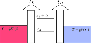
Figure 2: (Color online) Sketch of the quantum dot that is coupled to two external leads which are assumed to be at different temperatures $T\pm\delta T(t)/2$.

II Theoretical framework

II.1 Model Hamiltonian

In this work, we shall consider the case of a QD described by the Anderson model. It consists of a single localized orbital that is coupled to two external leads (see Fig. 2). The dot can accommodate up to two electrons with strong on-site interaction. The Hamiltonian takes the form

$$H = \sum_{\sigma}\varepsilon_{d}\;d^{\dagger}_{\sigma}d_{\sigma}+U\;d^{\dagger}_{\uparrow}d_{\uparrow}d^{\dagger}_{\downarrow}d_{\downarrow}\,$$

$$+ \sum_{{\bf k},\sigma}\sum_{\alpha=L,R}\left(\varepsilon_{\bf k}\;c^{\dagger}_{\alpha\bf k\sigma}c_{\alpha\bf k\sigma}+\Big{(}t_{\alpha{\bf k}}\;c^{\dagger}_{\alpha\bf k\sigma}d_{\sigma}+H.c.\Big{)}\right)\,,$$

where $d_{\sigma}$ is the annihilation operator of an electron with spin $\sigma$ in the dot, and $c^{\dagger}_{\alpha\bf k\sigma}$ is the creation operator of an electron with momentum $\bf k$ and spin $\sigma$ in lead $\alpha=\{L,R\}$. They satisfy the usual anticommutation relations: $\{d_{\sigma},d_{{\sigma}^{\prime}}^{\dagger}\}=\delta_{{\sigma}{\sigma}^{\prime}}$ and $\{c_{\alpha\bf k\sigma},c^{\dagger}_{\alpha^{\prime}\bf k^{\prime}\sigma^{\prime}}\}=(2\pi)^{3}\,\delta({\bf k-k^{\prime}})\,\delta_{\alpha\alpha^{\prime}}\,\delta_{\sigma\sigma^{\prime}}$. We treat the leads as having a constant density of states $\varrho(\omega)=\varrho_{0}=1/(2D)$, with $2D$ the bandwidth. The tunneling matrix is considered as being momentum independent, $t_{\alpha{\bf k}}=t_{\alpha}$. Its strength is characterized by the usual hybridization function $\Gamma_{\alpha}=\pi\varrho_{0}t_{\alpha}^{2}$. We define the total hybridization as $\Gamma=\sum_{\alpha=\{L,R\}}\Gamma_{\alpha}$. The dot itself supports a single orbital with energy $\varepsilon_{d}$ subject to the on-site Coulomb interaction $U$. Close to the electron-hole symmetric configuration, $\varepsilon_{d}\simeq-U/2$, the dot is in the Kondo regime, characterized by the Kondo energy scale which is defined as Haldane (1978)

$$T_{K}=\sqrt{U\,\Gamma\over 4}e^{\pi\varepsilon_{d}(\varepsilon_{d}+U)/\Gamma U}.$$ (10)

II.2 Currents and response functions

To compute the response functions, we need to define the charge and the heat currents. We introduce first the charge- and heat-transfer operators

$$Q_{\alpha}=Q^{(1)}_{\alpha} = e\sum_{\bf k,\sigma}c^{\dagger}_{\alpha\bf k\sigma}c_{\alpha\bf k\sigma},$$

$$K_{\alpha}=Q^{(2)}_{\alpha} = \sum_{\bf k,\sigma}(\varepsilon_{\bf k}-\mu_{\alpha})c^{\dagger}_{\alpha\bf k\sigma}c_{\alpha\bf k\sigma}\,,$$ (11)

and define the currents as time derivatives of the corresponding charge/heat operators:

$$I_{\alpha}^{(i)}=(-1)^{i+1}\frac{{\rm d}Q^{(i)}_{\alpha}}{{\rm d}t}\,.$$ (12)

Their explicit expressions can be obtained in terms of the equations of motion as:

$$I_{\alpha}^{(1)} = i\;\frac{e}{\hbar}\;\sum_{\bf k,\sigma}t_{\alpha}\;c^{\dagger}_{\alpha\bf k\sigma}d_{\sigma}+H.c.$$

$$I_{\alpha}^{(2)} = -\frac{i}{\hbar}\sum_{\bf k,\sigma}(\varepsilon_{\bf k}-\mu_{\alpha})t_{\alpha}\;c^{\dagger}_{\alpha\bf k\sigma}d_{\sigma}+H.c.\,.$$ (13)

To avoid a two-channel calculations, it is customary to perform a rotation of the $L/R$ basis to a new one $\{\alpha_{\bf k\sigma},\widetilde{\alpha}_{\bf k\sigma}\}$, defined by: $\alpha_{\bf k\sigma}=\xi_{L}\,c_{L\bf k\sigma}+\xi_{R}\,c_{R\bf k\sigma}$ and $\widetilde{\alpha}_{\bf k\sigma}=\xi_{R}\,c_{L\bf k\sigma}-\xi_{L}\,c_{R\bf k\sigma}$. This unitary transformation decouples the odd channel, $\widetilde{\alpha}_{{\mathbf{k}}{\sigma}}$, from the dot, so that the dot remains coupled only to the even channel, $\alpha_{{\mathbf{k}}{\sigma}}$. The coefficients are $\xi_{\alpha}=t_{\alpha}/\sqrt{t_{L}^{2}+t_{R}^{2}}$ and satisfy $\xi_{L}^{2}+\xi_{R}^{2}=1$. Following this unitary transformation, only the interacting part of the Hamiltonian $H_{\rm int}$ changes to $H_{\rm int}=t_{\rm eff}\;\sum_{\bf k,\sigma}\alpha^{\dagger}_{\bf k\sigma}d_{\sigma}+h.c.\,,$ with $t_{\rm eff}=\sqrt{t_{L}^{2}+t_{R}^{2}}$. In what follows we shall consider the perfectly symmetric dot, $t_{L}=t_{R}=t$. The currents, $I^{(i)}=(I^{(i)}_{L}-I^{(i)}_{R})/2$, transform accordingly, and under equilibrium conditions, $\mu_{L/R}=0$, in the new basis they are defined as:

$$I^{(1)} = i\,\frac{e\;t_{\rm eff}}{2\sqrt{2}\hbar}\;\sum_{\bf k,\sigma}\;\widetilde{\alpha}^{\dagger}_{\bf k\sigma}\,d_{\sigma}+H.c.$$ (14)

$$I^{(2)} = -i\,\frac{t_{\rm eff}}{2\sqrt{2}\,\hbar}\sum_{{\bf k},\sigma}\;\varepsilon_{\bf k}\,\left(\widetilde{\alpha}^{\dagger}_{\bf k\sigma}\,d_{\sigma}+H.c.\right)\,,$$ (15)

and are expressed in terms of the decoupled channel operators only. This allows us to obtain exact results for the response functions. The currents $I^{(i)}_{L/R}$ also have a symmetrical component, which gets subtracted out in the definition of $I^{(i)}$. Within the Kubo formalism, the generalized response functions $L_{ij}$ are given byhew

$$L_{ij}(t,t^{\prime})=-\frac{i}{\hbar}\Theta(t-t^{\prime})\langle[I^{(i)}(t),Q^{(j)}(t^{\prime})]\rangle\,,$$ (16)

where

$$Q^{(i)}=\frac{Q^{(i)}_{L}-Q^{(i)}_{R}}{2}\;.$$ (17)

We want to express $L_{ij}$ in terms of locally defined operators only, and for that we eliminate the charge operators. In Fourier space we obtain

$$L_{ij}(\omega)=-{T_{ij}(\omega)-T_{ij}(0)\over i\,\omega}\,,$$ (18)

with $T_{ij}(\omega)$ the Fourier transform of the generalized susceptibility:

$$T_{ij}(t,t^{\prime})=-\frac{i}{\hbar}\,\Theta(t-t^{\prime})\langle[I^{(i)}(t),I^{(j)}(t^{\prime})]\rangle.$$ (19)

Somewhat similar to the calculation of the ac conductance Sindel et al. (2005), the calculation of thermopower, $S(\omega)=S^{\prime}(\omega)+S^{\prime\prime}(\omega)$, reduces to the calculation of $A_{\rm d}(\omega)=-\rm Im\,G_{\rm d}^{\rm R}(\omega)/\pi$ - the spectral representation of the d-level operators in the dot (see Appendix B). In the present work $A_{\rm d}(\omega)$ shall be computed by using the Wilson numerical renormalization group approachKrishna-murthy et al. (1980a, b); Bulla et al. (2008) (NRG) as implemented in the Flexible-NRG code. Bud Throughout the NRG calculation, the Wilson ratio was fixed to $\Lambda=2$, and we have kept on average 4000 multiplets at each iteration.

III Ac thermopower

Let us now focus on the calculations of the response functions $L_{ij}$ and the ac thermopower $S(\omega)$. In general, $L_{ij}(\omega)$ are complex functions of $\omega$, as their imaginary parts capture retardation effects due to the external excitation. The full $\omega$ dependence of the ${\rm Re}\,L_{ij}(\omega)$ acquires a relatively compact expression in terms of the spectral representation of the d-level:

$$\textrm{Re}\,L_{ij}(\omega)=\frac{t_{\rm eff}^{2}}{2\omega\hbar}\left(-\frac{e}{\hbar}\right)^{4-i-j}\varrho_{0}\int\rm d\omega^{\prime}\left\{\textrm{Im}G_{d}^{R}(\omega^{\prime})\right.$$

$$\left[(\omega^{\prime}-\omega)^{i+j-2}\Theta_{\omega^{\prime}-\omega}f(\omega^{\prime}-\omega)+\right.$$

$$+(\omega^{\prime}+\omega)^{i+j-2}\Theta_{\omega^{\prime}+\omega}f(\omega^{\prime})-$$

$$-(\omega^{\prime}-\omega)^{i+j-2}\Theta_{\omega^{\prime}-\omega}f(\omega^{\prime})$$

$$\left.\left.-(\omega^{\prime}+\omega)^{i+j-2}\Theta_{\omega^{\prime}+\omega}f(\omega^{\prime}+\omega)\right]\right\}\,,$$

with $\Theta_{\omega}=\Theta(D-|\omega|)$ and $f(\omega)$ the Fermi-Dirac distribution. To get the ac conductance Sindel et al. (2005), the high energy cut-off $D$ can be safely taken to infinity, as $L_{11}$ remains a regular function. This is not the case for $L_{12}$ which diverges at large frequencies when $D\to\infty$, so it is compulsory to have a finite bandwidth for the conduction electrons. To get the imaginary part of $L_{ij}$, the use of the Hilbert transform is unavoidable. We first compute ${\rm Re}\,L_{ij}$, and then ${\rm Im}\,L_{ij}$ is obtained by a Kramers-Krönig(KK) transformation

$$\textrm{Im}\,L_{ij}(\omega)=-\frac{1}{\pi}\int_{-\infty}^{+\infty}\frac{\textrm{Re}\,L_{ij}(\omega^{\prime})}{\omega^{\prime}-\omega}\rm d\omega^{\prime}$$ (21)

Although Eq. (III) looks cumbersome, we can interpret it in terms of inelastic tunneling processes and see these correlation functions as rates by which the system absorbs or emits photons Basset et al. (2012) at frequencies $\omega$. Further details on how to compute $L_{ij}$ are presented in Appendix B. With $L_{ij}$ at hand, $S(\omega)$ can be obtained by using Eq. (7). By symmetry, $S^{\prime}(\omega)=S^{\prime}(-\omega)$, is an even function of frequency, while $S^{\prime\prime}(\omega)=-S^{\prime\prime}(-\omega)$, is an odd function. The full $\omega$ and $T$ dependence for $S(\omega)$ is displayed in Figs.  3 (a)- 3(f), while in Figs.  3(g) and  3(h) a cut at constant temperature $T=0.1\,\Gamma$ is presented.

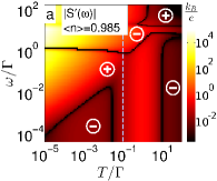
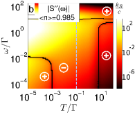
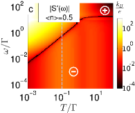
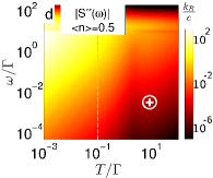
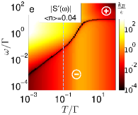
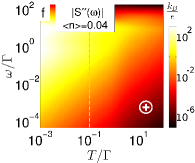
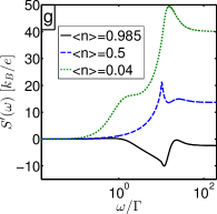
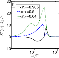
Figure 3: (Color online) Density plots for the real and imaginary parts of the thermopower in the $(T,\omega)$ plane: (a), (b) Kondo regime, (c), (d) mixed valence regime, and (e), (f) empty orbital regime. Panels (g) and (h) represent the thermopower at $T=0.1\,\Gamma$ for positive $\omega$ along the dashed lines in the density plots. The darker lines are the locations of the zeros, and mark the positions where the thermopower changes sign. The $(\pm)$ symbols indicate the signs of $S(\omega)$. The NRG parameters used are $U/\Gamma=10$, $\varepsilon_{d}/\Gamma=-4\,(n=0.985)$, $\varepsilon_{d}/\Gamma=-0.2\,(n=0.5)$ and $\varepsilon_{d}/\Gamma=5\,(n=0.04)$.

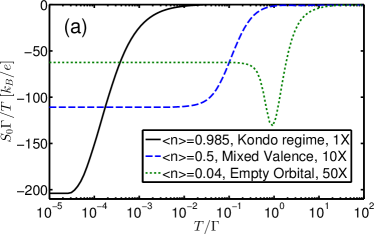
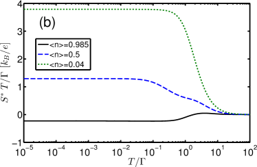
Figure 4: (Color online) (a) The dc-thermopower $S_{0}=S(\omega=0)$ as function of temperature in different regimes. (b) Temperature dependence of $S^{*}=S(\omega\gg D)$.

In Figs.  3(a)- 3(b), we represent the results for $S(\omega,T)$ when the system is in the Kondo regime, where $\epsilon_{d}\simeq-U/2$, and $\langle n\rangle\simeq 1$. Figs.  3(c) and  3(d) present results for $S(\omega,T)$ in the mixed valence regime with $\langle n\rangle=0.5$, while Figs.  3(e) and  3(f) show $S(\omega,T)$ in the empty orbital limit, $\langle n\rangle\ll 1$. By symmetry, when $1<n<2$, the thermopower has the same magnitude, but opposite sign, as the role of particles and holes is inverted. At the electron-hole symmetric point, i.e., $n=1$, the particles and holes move together in the same direction under the temperature gradient, and the thermopower vanishes exactly.

At very small frequencies and temperatures, $\{\omega,T\}\to 0$, only the quasiparticles very close to the Fermi surface give a contribution to the currents flowing through the device, so this limit can be understood in terms of the Fermi-liquid picture. Nozières (1974) The Fermi-liquid scale $\Omega_{F}$, is controlled by either $T_{K}$ within the Kondo regime, or by $\Gamma$ itself otherwise. When $\{\omega,T\}\ll\Omega_{F}$, the frequency dependence of $S(\omega)$ is captured by a simple analytical expression

$$S(\omega,T)=S_{0}(T)+b^{\prime}(T)\,{\omega}^{2}+i\,b^{\prime\prime}(T)\,{\omega}+\dots\,.$$ (22)

Here $S_{0}(T)<0$, is the dc-thermopower, while $b^{\prime}$ and $b^{\prime\prime}$ are some coefficients that depend on temperature. In the Kondo regime, $\{b^{\prime}(T),b^{\prime\prime}(T)\}\sim 1/T$. In our convention, positive (negative) $S_{0}$ corresponds to the situation when charge and heat currents flow in the same (opposite) directions. At some intermediate frequencies, $\omega\sim T$, $S^{\prime}(\omega)$ changes sign and becomes positive. In the Kondo regime, there is another change of sign at a larger, almost constant frequency $\omega_{2}\simeq\Gamma$, and $S^{\prime}$ becomes negative in the $\omega\gg D$ limit. The sign of $S_{0}(T)$ can be associated with the type of dominant carriers in the system at that particular energy: hole like carriers correspond to $S_{0}>0$, and particle like carriers to $S_{0}<0$. The first sign change in $S_{0}(T)$ can be understood as follows: At $T\simeq 0$, the Kondo peak is weighted towards positive energies (for $n<1$), but as temperature increases, it is pulled towards the negative energy region. Thus, the quantum dot shifts from having predominantly particle carriers, to having predominantly hole carriers in the window $\sim T$ that contributes to the transport. Whenever the average entropy carried inside this window becomes zero, the thermopower vanishes. At a finite frequency $\omega$, inelastic tunneling processes in a window $\sim 2\omega$ around the Fermi level give additional contributions to the transport, see Eq. (III). The picture gets more complicated by the existence of retardation effects, which lead to finite imaginary parts in the response functions, and consequently affect the zeros of the thermopower. The high-frequency features in Fig. 3 at energies $\omega\sim\{U,D\}$ can be associated with Hubbard charging, and eventually band-edge effects. In Fig. 4, we display the temperature dependence of $S_{0}(T)$ and $S^{*}(T)$. It has been already shown Costi and Hewson (1993) that in the Kondo regime, when $T\ll T_{K}$, $S_{0}$ depends linearly on $T$, $S_{0}\propto T$. This observation carries over to the mixed valence and empty orbital regimes too, as long as $T\ll\Gamma$. In the opposite limit, $T\gg T_{K}$, $S_{0}$ shows a change of sign at some large temperature, and then decays towards zero.

In the large-frequency limit $\omega\gg D$, $S^{*}$ can be evaluated simply as

$$S^{*}(T)=\frac{1}{T}\frac{L_{12}^{*}}{L_{11}^{*}}.$$ (23)

with $L_{ij}^{*}$ some temperature-dependent coefficients, discussed in Appendix B (see Eq. (34)). As $\omega\gg D$, all states are involved in transport, so that the only energy scale that survives is the bandwidth itself (as long as $\{T_{K},U\}\ll D$). Therefore, we expect the features of $S^{*}(T)$ to carry information only on $D$ itself. In the small-temperature limit, $T\to 0$, the $L_{ij}^{*}$’s become constants, so a divergent behavior $S^{*}\propto 1/T$ emerges in this limit. This is clearly visible in Fig. 4 (b), where $S^{*}T$ becomes constant when $T\ll\Gamma$. At intermediate temperatures, $\Gamma<T<D$, $S^{*}$ decreases significantly, and vanishes in the in large $T$ limit.

In what follows we shall focus on the strongly correlated regime. When $\{\omega,T\}\leq T_{K}$, a clear universal behavior emerges as $S(\omega)$ depends exclusively on the $T/T_{K}$ and $\omega/T_{K}$ ratios.

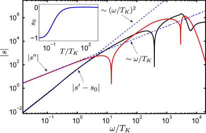
Figure 5: (Color online) Universal scaling functions for a filling $\left<n\right>=0.95$ for a fixed temperature, $T=0.02\;T_{K}$. In the inset, we represent the $s_{0}$ universal function.

It was found previouslyCosti and Zlatić (2010) that as long as $T\ll T_{K}$,

$$s_{0}(T/T_{K}) = \Big{(}\frac{e}{\pi\gamma\,T}\Big{)}S_{0}(T)\,\tan\delta_{0}$$ (24)

$$= \frac{e}{k_{B}}\Big{(}\frac{T_{K}}{T}\Big{)}S_{0}(T)\,\left(\frac{\tan\delta_{0}}{{\tilde{\gamma}}}\right)$$

is a universal function that scales with $T/T_{K}$ up to a filling-dependent phase factor. Here, $\delta_{0}$ is the phase shift at the Fermi level, $\delta_{0}=\pi\langle n\rangle/2$, with $\langle n\rangle$ the average occupation of the dot, $\gamma$ is the specific-heat coefficient of the quantum dot which is filling dependent, and ${\tilde{\gamma}}=\pi\gamma\,T_{K}/k_{B}$ is a dimensionless quantity of the order 1. In the inset of Fig. 5 we represent $s_{0}(T/T_{K})$ as a function of $T/T_{K}$ for a filling $\langle n\rangle=0.95$. We extend this analysis to finite frequencies where a similar behavior emerges, as the ac thermopower can be expressed as:

$$S(\omega,T)={k_{B}\over e}\Big{(}{T\over T_{K}}\Big{)}\,s(\omega/T_{K},T/T_{K})\,{\tilde{\gamma}}\,\cot(\delta_{0})\,.$$ (25)

The universal scaling function $s$ depends on $\omega/T_{K}$ and $T/T_{K}$ only. A sketch with the frequency dependence is presented in Fig. 1, while in Fig. 5 we represent the exact numerical calculation for the frequency dependence of $|s|$. In the Fermi-liquid regime, $\{\omega,T\}\ll T_{K}$, simple analytical expressions can approximate the real and imaginary parts of $s$:

$$s^{\prime}\Big{(}{\omega\over T_{K}},{T\over T_{K}}\Big{)} = s_{0}\Big{(}{T\over T_{K}}\Big{)}+\alpha^{\prime}\Big{(}{\omega\over T_{K}}\Big{)}^{2}\Big{(}{T_{K}\over T}\Big{)}^{2}+\dots,$$

$$s^{\prime\prime}\Big{(}{\omega\over T_{K}},{T\over T_{K}}\Big{)} = \alpha^{\prime\prime}\Big{(}{\omega\over T_{K}}\Big{)}\Big{(}{T_{K}\over T}\Big{)}^{2}+\dots.$$ (26)

with $\alpha^{\prime}$ and $\alpha^{\prime\prime}$ some coefficients $\sim 1$. The $s^{\prime}\sim\omega^{2}$ frequency dependence can be related to the virtual Kondo transitions from the singlet ground state to the excited states. Glazman and Pustilnik (2003) These transitions give for the imaginary part of the T-matrix: $\textrm{Im}\,{\rm T}(\omega,T)\propto 1-{(3\,\omega^{2}+\pi^{2}T^{2})}/{T_{K}^{2}}$, when $\{\omega,T\}\ll T_{K}$, which in turn introduces corrections of the order $\sim\omega^{2}$ and $\sim T^{2}$ in the response functions $\textrm{Re}\,L_{ij}$. Simple analytics then show that $s^{\prime}\sim\omega^{2}/T^{2}$. Then, by Hilbert transform, $s^{\prime\prime}$ is linear in frequency. This scaling for $s$ extends up to frequencies of the order of $\omega\sim T_{K}$, followed by a sign change at some particular frequencies $\omega_{i}$. At very large frequencies $\omega\gg T_{K}$, $s^{\prime}$ becomes a constant, while $s^{\prime\prime}\to 0$.

IV Concluding Remarks

We have studied the finite-frequency thermopower of a quantum dot described by the Anderson model. For that we have first constructed a general framework which allowed us to investigate in a non-perturbative manner the ac thermopower. When calculating the ac conductance Sindel et al. (2005), it is safe to take the bandwidth $D\to\infty$, but when we address the problem of the ac thermopower, it is compulsory to keep $D$ finite. Although $S(\omega)$ presents a relatively rich structure that includes several sign changes, in the Fermi liquid regime a simple analytical expression is able to capture its behavior over a broad range of temperatures and frequencies. In the Kondo regime, the ac thermopower is characterized by a universal function that we have determined numerically. We have also found that the $S_{0}$ and $S^{*}$ have a markedly different behavior in the low-temperature limit.

Appendix A Green’s Functions

Within the L/R basis transformation, one channel becomes decoupled, and can be treated as a non-interacting one. It is simply described by the non-interacting Hamiltonian $H_{0}=\sum_{\bf k,\sigma}\varepsilon_{\bf k}\;\widetilde{\alpha}^{\dagger}_{\bf k\sigma}\,\widetilde{\alpha}_{\bf k\sigma}$. In what follows, we shall fix the chemical potential to zero. The non-equilibrium evolution of the system is described by the conduction electron Green’s function: $g_{\bf k\sigma}(t-t^{\prime})=-i\langle{\cal T_{C}}\widetilde{\alpha}_{\bf k\sigma}(t)\widetilde{\alpha}^{\dagger}_{\bf k\sigma}(t^{\prime})\rangle$, where $\cal T_{C}$ is the time ordering operator on the Keldysh contour. Within this language, we can define four Green’s functions. Two combinations define the greater and lesser components

$$g^{>}_{\bf k\sigma}(t-t^{\prime}) = -i\langle\widetilde{\alpha}_{\bf k\sigma}(t)\,\widetilde{\alpha}^{\dagger}_{\bf k\sigma}(t^{\prime})\rangle,$$

$$g^{<}_{\bf k\sigma}(t-t^{\prime}) = i\langle\widetilde{\alpha}^{\dagger}_{\bf k\sigma}(t^{\prime})\,\widetilde{\alpha}_{\bf k\sigma}(t)\rangle,$$ (27)

while the other two define the time and anti-time ordered ones: $g^{t}_{\bf k\sigma}(t-t^{\prime})=-i\langle{\cal T}\,\widetilde{\alpha}_{\bf k\sigma}(t)\,\widetilde{\alpha}^{\dagger}_{\bf k\sigma}(t^{\prime})\rangle$, and $g^{\tilde{t}}_{\bf k\sigma}(t-t^{\prime})=-i\langle\tilde{\cal T}\widetilde{\alpha}_{\bf k\sigma}(t)\,\widetilde{\alpha}^{\dagger}_{\bf k\sigma}(t^{\prime})\rangle$. Here ${\cal T}$ and $\cal\tilde{T}$ are the time and anti-time ordering operators. We also introduce the retarded and the advanced Green’s functions, which are defined in the usual way:

$$g^{A}_{\bf k\sigma}(t-t^{\prime}) = i\Theta(t^{\prime}-t)\langle\{\widetilde{\alpha}_{\bf k\sigma}(t),\widetilde{\alpha}^{\dagger}_{\bf k\sigma}(t^{\prime})\}\rangle,$$

$$g^{R}_{\bf k\sigma}(t-t^{\prime}) = -i\Theta(t-t^{\prime})\langle\{\widetilde{\alpha}_{\bf k\sigma}(t),\widetilde{\alpha}^{\dagger}_{\bf k\sigma}(t^{\prime})\}\rangle.$$ (28)

We are interested in the momentum integrated Green’s function $g_{\sigma}(\omega)=\sum_{\bf k}g_{\bf k{\sigma}}(\omega)$, as these are the only quantities that explicitly enter the expression for the ac thermopower. Here, we consider the simplest situation of a dispersionless electronic band with a band cutoff D. It is characterized by a constant density of states $N(\omega)=1/(2D)\,\Theta(D-|\omega|)=N(0)\,\Theta_{\omega}$, with $N(0)=1/(2D)$, the DOS at the Fermi level and $\Theta_{\omega}=\Theta(D-|\omega|)$. Then, the momentum integrated Green’s function have relatively simple analytical expressions Körting : $g^{>}_{\sigma}(\omega)=-2\pi i\,(1-f(\omega))\,N(0)\,\Theta_{\omega}$, $g^{<}_{\sigma}(\omega)=2\pi i\,f(\omega)\,N(0)\,\Theta_{\omega}$ and $\textrm{Im}\,g^{A}_{\sigma}(\omega)=-\textrm{Im}\,g^{R}_{\sigma}(\omega)=i\,\pi N(0)\Theta_{\omega}$. Usually, $\textrm{Re}\,g^{R/A}$ is neglected in the large-bandwidth limit, but as long as we are interested in the response functions $L_{ij}$ in the large $\omega>D$ limit, its contribution becomes important.

Appendix B Current Correlations and the dynamical transport coefficients

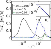
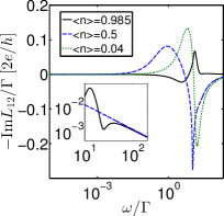
Figure 6: (Color online) The imaginary part of the dynamical coefficients $L_{ij}(\omega)$ as function of frequency. The inset shows the asymptotic $\sim 1/\omega$ behavior in the large-$\omega$ limit in the Kondo regime for $\langle n\rangle=0.985$. The temperature was fixed to T=$10^{-5}\Gamma$.

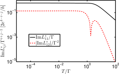
Figure 7: (Color online) The temperature dependence of $L_{ij}^{*}$ in the Kondo regime. The results are obtained by using the sum rule expression, Eq. (34).

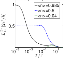
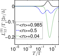
Figure 8: (Color online). The temperature dependence of $\rm Re\,L_{ij}^{(0)}$. Here $L_{11}^{(0)}$ can be identified with the dc-conductance itself.

To get the dynamical transport coefficients, we need to compute the retarded response functions defined in Eq. (19), with the current operators defined in Eqs. (14) and (15). In the even/odd basis, one channel becomes decoupled and the charge current correlator $T_{11}$ can be evaluated as:

$$T_{11}(t-t^{\prime})=\Theta(t-t^{\prime})\frac{e^{2}}{\hbar^{3}}\frac{t_{\rm eff}^{2}}{4}\sum_{\bf k,\sigma}$$

$$\left\{G_{d}^{>}(t-t^{\prime})g^{<}_{\bf k\sigma}(t^{\prime}-t)-G_{d}^{<}(t-t^{\prime})g^{>}_{\bf k\sigma}(t^{\prime}-t)-\right.$$

$$\left.-G_{d}^{<}(t^{\prime}-t)g^{>}_{\bf k\sigma}(t-t^{\prime})-G_{d}^{>}(t^{\prime}-t)g^{<}_{\bf k\sigma}(t-t^{\prime})\right\},$$ (29)

which gives for $L_{11}$ defined in Eq. (18) a relatively compact expression:

$$\textrm{Re}\,L_{11}(\omega)=-\frac{t_{\rm eff}^{2}}{2\omega}\frac{e^{2}}{\hbar^{3}}\varrho_{0}\int\rm d\omega^{\prime}\left\{\textrm{Im}G_{d}^{R}(\omega^{\prime})\left[\right.\right.$$

$$\Theta_{\omega^{\prime}-\omega}f(\omega^{\prime}-\omega)+\Theta_{\omega^{\prime}+\omega}f(\omega^{\prime})-\Theta_{\omega^{\prime}-\omega}f(\omega^{\prime})-$$

$$\left.\left.-\Theta_{\omega^{\prime}+\omega}f(\omega^{\prime}+\omega)\right]\right\}.$$ (30)

Notice that within the present formalism, we can identify $\rm Re\,L_{11}(\omega)$ with the real part of the ac conductance $G(\omega)$. Sindel et al. (2005) A similar expression can be derived for $T_{12}(t,t^{\prime})$, which in the Fourier space becomes:

$$T_{12}(\omega)=-\frac{t_{\rm eff}^{2}}{4}\frac{e}{\hbar^{3}}\sum_{\bf k,\sigma}\varepsilon_{\bf k}\int\frac{\rm d\omega^{\prime}}{2\pi}\left\{G_{d}^{R}(\omega+\omega^{\prime})g_{\bf k\sigma}^{<}(\omega^{\prime})\right.$$

$$+G_{d}^{<}(\omega+\omega^{\prime})g_{\bf k\sigma}^{A}(\omega^{\prime})+G_{d}^{>}(\omega^{\prime})g_{\bf k\sigma}^{R}(\omega+\omega^{\prime})+$$

$$\left.+G_{d}^{A}(\omega^{\prime})g_{\bf k\sigma}^{>}(\omega+\omega^{\prime})\right\}.$$ (31)

Subtracting the $T_{12}(\omega=0)$ term and dividing by $-i\omega$, the real part of $L_{12}$ is obtained as:

$$\textrm{Re}\,L_{12}(\omega)=\frac{t_{\rm eff}^{2}}{2\omega}\frac{e}{\hbar^{2}}\varrho_{0}\int\rm d\omega^{\prime}\left\{\textrm{Im}G_{d}^{R}(\omega^{\prime})\left[\right.\right.$$

$$(\omega^{\prime}-\omega)\Theta_{\omega^{\prime}-\omega}f(\omega^{\prime}-\omega)+(\omega^{\prime}+\omega)\Theta_{\omega^{\prime}+\omega}f(\omega^{\prime})-$$

$$\left.\left.-(\omega^{\prime}-\omega)\Theta_{\omega^{\prime}-\omega}f(\omega^{\prime})-(\omega^{\prime}+\omega)\Theta_{\omega^{\prime}+\omega}f(\omega^{\prime}+\omega)\right]\right\}.$$ (32)

In these expressions, $L_{ij}$ depends explicitly on the retarded localized d-level Green’s function $\rm G_{d}^{R}(\omega)$. This quantity shall be computed exactly by using the NRG method. In this way, Eqs. (B) and (B) are the exact expressions for the real parts of the Onsager transport coefficients, and no approximation of any kind was used so far. The ac thermopower depends not only on the real, but also on the imaginary parts of $L_{ij}$. Actually their imaginary parts give the main contribution in the large-frequency limit. To obtain them, we use the Kramers-Krönig relations, Eq. (21). In the ac limit, when $\omega$ is the largest energy scale ($\omega\gg D$), we can simplify considerably the calculation by noticing that

$$\textrm{Im}\,L_{ij}(\omega)\simeq\frac{L_{ij}^{*}}{\omega}$$ (33)

with $L_{ij}^{*}$ some coefficients,

$$L_{ij}^{*}=\frac{1}{\pi}\int_{-\infty}^{+\infty}\textrm{Re}\,L_{ij}(\omega^{\prime})\rm d\omega^{\prime},$$ (34)

which are thus determined as the sum rule of dynamical quantities. Xu et al. (2011) In Fig. 6 we represent the imaginary parts of $L_{ij}$ in the Kondo regime, as computed by doing the KK transformations of Eq. (B) and (B). The insets display the large-frequency behavior, which indicates that our approximation, Eq. (33), is indeed correct. The temperature dependence of $L_{ij}^{*}$ is displayed in Fig. 7.

In the small-frequency limit, $\omega\rightarrow 0$, the calculation can be simplified again. Introducing the notation $\textrm{Re}\,L_{ij}^{(0)}=\textrm{Re}L_{ij}\,(\omega\rightarrow 0)$, we notice that Eqs. (B) and (B) reduce considerably to

$$\textrm{Re}\,L_{ij}^{(0)}=\frac{t_{\rm eff}^{2}}{\hbar}\left(-\frac{e}{\hbar}\right)^{4-i-j}\varrho_{0}\times\,\\ \int\rm d\tilde{\omega}\,\left(\tilde{\omega}^{i+j-2}\textrm{Im}G_{d}^{R}(\tilde{\omega})\frac{\partial f(\tilde{\omega})}{\partial\tilde{\omega}}\right).$$ (35)

Here, $\textrm{Re}\,L_{11}^{(0)}$ is the dc-conductance itself. Its temperature dependence is displayed in Fig. 8. As expected in the $T\rightarrow 0$ limit, $\textrm{Re}\,L_{11}^{(0)}$ shows the usual Kondo behavior, as the system is close to the unitary limit. From Eqs. (35) and (7) one can notice that the thermopower has the form of an average entropy $-\left<\epsilon-\mu\right>/(eT)$ carried per particle/hole across the quantum dot. Thus, for the case of perfect particle-hole symmetry, the thermopower becomes zero. This form can also be used to justify the $1/T$ dependence of $S^{*}$ (see Fig. 3).

References

- Sales et al. (1996) B. C. Sales, D. Mandrus, and R. K. Williams, Science 272, 1325 (1996).
- Snyder and Toberer (2008) G. J. Snyder and E. S. Toberer, Nat. Mater. 7, 104 (2008).
- Heremans et al. (2008) J. P. Heremans, V. Jovovic, E. S. Toberer, A. Saramat, K. Kurosaki, A. Charoenphakdee, S. Yamanaka, and G. J. Snyder, Science 321, 554 (2008).
- Humphrey et al. (2002) T. E. Humphrey, R. Newbury, R. P. Taylor, and H. Linke, Phys. Rev. Lett. 89, 116801 (2002).
- Harman et al. (2002) T. C. Harman, P. J. Taylor, M. P. Walsh, and B. E. LaForge, Science 297, 2229 (2002).
- Wang et al. (2008) R. Y. Wang, J. P. Feser, J.-S. Lee, D. V. Talapin, R. Segalman, and A. Majumdar, Nano Letters 8, 2283 (2008).
- Svensson et al. (2012) S. F. Svensson, A. I. Persson, E. A. Hoffmann, N. Nakpathomkun, H. A. Nilsson, H. Q. Xu, L. Samuelson, and H. Linke, New Journal of Physics 14, 033041 (2012).
- Beenakker and Staring (1992) C. W. J. Beenakker and A. A. M. Staring, Phys. Rev. B 46, 9667 (1992).
- Boese and Fazio (2001) D. Boese and R. Fazio, Europhys. Lett. 56, 576 (2001).
- Scheibner et al. (2005) R. Scheibner, H. Buhmann, D. Reuter, M. N. Kiselev, and L. W. Molenkamp, Phys. Rev. Lett. 95, 176602 (2005).
- Costi and Zlatić (2010) T. A. Costi and V. Zlatić, Phys. Rev. B 81, 235127 (2010).
- Roura-Bas et al. (2012) P. Roura-Bas, L. Tosi, A. A. Aligia, and P. S. Cornaglia, Phys. Rev. B 86, 165106 (2012).
- Trocha and Barnaś (2012) P. Trocha and J. Barnaś, Phys. Rev. B 85, 085408 (2012).
- Donsa et al. (2013) S. Donsa, S. Andergassen, and K. Held, arXiv:1308.4882 (2013).
- Lim et al. (2013) J. S. Lim, R. López, and D. Sánchez, Phys. Rev. B 88, 201304 (2013).
- Sindel et al. (2005) M. Sindel, W. Hofstetter, J. von Delft, and M. Kindermann, Phys. Rev. Lett. 94, 196602 (2005).
- Blanter and Sukhorukov (2000) Y. M. Blanter and E. V. Sukhorukov, Phys. Rev. Lett. 84, 1280 (2000).
- Moca et al. (2011) C. P. Moca, I. Weymann, and G. Zarand, Phys. Rev. B 84, 235441 (2011).
- Kogan et al. (2004) A. Kogan, S. Amasha, and M. A. Kastner, Science 304, 1293 (2004).
- Basset et al. (2012) J. Basset, A. Y. Kasumov, C. P. Moca, G. Zaránd, P. Simon, H. Bouchiat, and R. Deblock, Phys. Rev. Lett. 108, 046802 (2012).
- Shastry (2006) B. S. Shastry, Phys. Rev. B 73, 085117 (2006).
- Shastry (2009) B. S. Shastry, Reports on Progress in Physics 72, 016501 (2009).
- Xu et al. (2011) W. Xu, C. Weber, and G. Kotliar, Phys. Rev. B 84, 035114 (2011).
- (24) Mahan, G. D., Many-Particle Physics (Kluwer Academic, New York, 2000) .
- Luttinger (1964) J. M. Luttinger, Phys. Rev. 135, A1505 (1964).
- Haldane (1978) F. D. M. Haldane, Phys. Rev. Lett. 40, 416 (1978).
- (27) A. C. Hewson, The Kondo Problem to Heavy Fermions (Cambridge University Press, Cambridge, 1993) .
- Krishna-murthy et al. (1980a) H. R. Krishna-murthy, J. W. Wilkins, and K. G. Wilson, Phys. Rev. B 21, 1003 (1980a).
- Krishna-murthy et al. (1980b) H. R. Krishna-murthy, J. W. Wilkins, and K. G. Wilson, Phys. Rev. B 21, 1044 (1980b).
- Bulla et al. (2008) R. Bulla, T. A. Costi, and T. Pruschke, Rev. Mod. Phys. 80, 395 (2008).
- (31) We used the open-access Budapest Flexible DM-NRG code, http://www.phy.bme.hu/~dmnrg/; O. Legeza, C. P. Moca, A. I. Tóth, I. Weymann, G. Zaránd, arXiv:0809.3143 (2008) (unpublished) .
- Nozières (1974) P. Nozières, Journal of Low Temperature Physics 17, 31 (1974).
- Costi and Hewson (1993) T. A. Costi and A. C. Hewson, Journal of Physics: Condensed Matter 5, L361 (1993).
- Glazman and Pustilnik (2003) L. Glazman and M. Pustilnik, New Directions in Mesoscopic Physics (Towards Nanoscience), NATO Science Series, 125, 93 (2003).
- (35) V. Körting, Ph.D. thesis, Karlsruhe University, 2007 .