Second Harmonic Generation in Gapped Graphene

Abstract

The second-order nonlinear optical susceptibility $\Pi^{(2)}$ for second harmonic generation is calculated for gapped graphene. The linear and second-order nonlinear plasmon excitations are investigated in context of second harmonic generation (SHG). We report a red shift and an order of magnitude enhancement of the SHG resonance with growing gap, or alternatively, reduced electro-chemical potential.

I Introduction

Since the discovery of second harmonic generation (SHG) by Franken et al. and the demonstration of the first working laser by Maiman in early 60-x, various nonlinear optical techniques has received considerable attentionboyd . At the hear of those techniques lays the response to $n-$power of the optical filed $\Pi^{(n)}$, which , in essence, is the multi-point correlation function between the electrons of the probed substancemukamel . For instance, $\Pi^{(2)}$ describes various two-wave mixing such as SHG, sum and difference frequency generation (SFG,DFG) and linear electro-optical effects (Pockets). Those are of great importance in areas of integrated optics and optical communication, SFG based frequency-tunable visible lasers and DFG based optical parametric oscillators boyd . Typical value of $\Pi^{(2)}$ is of the order of $\sim\,1.67\times 10^{-12}m/V$. Various groups 1467 ; khurgin ; rosencher ; yoo ; harshman ; shaw ; seto ; cai demonstrated substantial enhancement of $\Pi^{(2)}$ for an asymmetric quantum well (QW), asymmetric double quantum well (DQW) and several bond-altering dipolar structures. In addition, there are quite a few paperskuwatsuka ; tsang ; fejer ; west dealing with the calculation of $\Pi^{(2)}$ for a single QW biased by an electric field.

SHG is a powerful optical tool for probing surfaces, thin filmsshen , multilayer graphenebykov as well as hetero interfaces such as two dimensional electron gasstern of centrosymmetric materials. In the dipole approximation, SHG is prohibited in the bulk of such materials, while at surfaces and interfaces the central symmetry is broken. For the two dimensional electron gas, SHG gives two orders of magnitude larger signal when compared with surfaces. Recently, an additional two orders of magnitude enhancement of the SHG signal in graphene compared with $GaAs$ two dimensional electron gas was predictedmikhailov , as shown in Fig.1. The author also reported an order of magnitude larger linear response in that system.

A typical graphene-based SHG experimental set-up involves specular light reflection in the wave length range of $730-830\;nm$. Reflected SHG radiation is spectrally selected and quadratic dependence of the signal on the incoming pulse intensity must be assuredbykov . The inversion symmetry between A and B sub-lattices in graphene can be broken by external fields causing so-called field induced SHGpan . On the level of graphene electronic spectra, the external influence opens up a gap. Examples of such Dirac cone perturbation are multilayer epitaxially grown grapheneohta , circularly polarized lightkibis and underlying substrategiovannetti . On one hand, the gap makes graphene behave more like conventional 2DEG thus lowering the SHG intensity. On the other hand, the field induced SHG boosts the signal. In this paper we investigate the interplay between these two effects schematically as shown in Fig.2.

Our paper focuses on gapped graphene. As will be discussed later, the gap in the graphene electronic spectrum means broken inversion symmetry, thereby promising enhanced second-order response. The resonances in linear density-density response are known as plasmons. We shall demonstrate the existence of similar plasmon-like resonances in the second-order response, in particular the part corresponding to SHG.

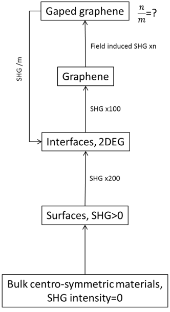
Figure 1: (Color online) Hierarchy of SHG enhancement.

II Model for Gapped Graphene

In the low energy regime near the Dirac points, the electronic spectrum of graphene exhibits the familiar linear dispersion with zero energy gap at the two Dirac points ($\mathbf{K},\mathbf{K}^{\prime}$). Opening a gap in the spectrum of graphene generally involves breaking the underlying inversion symmetry. There are several ways in which the symmetry might be broken. These include coupling with a quantized circularly polarized field, breaking of the sub-lattice symmetry, spin-orbit coupling via the Rashba interaction, reduction in dimension leading edge effects in zigzag nano-ribbons or confinement in armchair nano-ribbons. For small deviation $\mathbf{k}$ in the electron momentum from the Dirac points, the tight-binding model reduces to the eigenvalue equation $H_{g}|{\lambda}\rangle={E}|{\lambda}\rangle$, where the Hamiltonian is given by

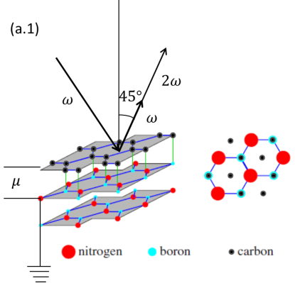
Figure 2: (Color online) Panel (a.1) schematic of the SHG specular reflection experiment

$$H_{g}=\left(\begin{array}[]{cccc}E_{g}/2&\hbar v_{F}k^{*}&0&0\\ \hbar v_{F}k&-E_{g}/2&0&0\\ 0&0&-E_{g}/2&-\hbar v_{F}k^{*}\\ 0&0&-\hbar v_{F}k&E_{g}/2\end{array}\right)\$$ (1)

where $k=k_{x}+ik_{y}$ is the complex wave-vector, $v_{F}$ is the Fermi velocity and the electronic states for the A,B sublatices are $\langle\mathbf{k}|{\lambda}\rangle=[\psi_{A}({\bf k}),\psi_{B}({\bf k}),-\psi^{\prime}_{A}({\bf k}),-\psi^{\prime}_{B}({\bf k})]$. The corresponding eigenvalues yield the conduction and valence bands shown schematically in Fig. 2:

$${E}_{\pm}=\pm\sqrt{E^{2}_{g}/4+(\hbar v_{f}k)^{2}}\$$ (2)

Here $E_{g}$ is the energy gap at $k=0$. The alternating sign of $E_{g}$ in Eq.(1) indicates broken symmetry between the A and B sub-lattices. In the next section, we employ this feature in order to generate second-order nonlinear polarization.

III Linear and second order-response of gapped graphene subjected to a harmonic potential

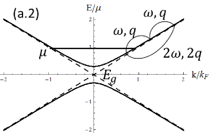
Figure 3: (Color online) Intraband induced SHG in gaped graphene in the long wavelength approximation.

We now consider the dynamics of graphene interaction with an oscillating single-mode electromagnetic field described by the potential $\Phi({\bf r},t)=\Phi_{{\bf q}\omega}e^{i({\bf q\cdot r}-\omega t)}+c.c.$. In this section, we derive a formal expression for the response function due to an external perturbation up to second order and further process it in the long wavelength approximation. Perturbative treatment of the density matrix suits best for that purpose. The reduced density operator $\hat{\rho}$ satisfies the equation of motion:

$$i\hbar\frac{\partial\hat{\rho}}{\partial t}=[H_{g}+H_{int},\hat{\rho}]$$ (3)

$$H_{int}=-e\Phi({\bf r},t)\ .$$

The external field is turned on adiabatically, i.e.,

$$\begin{cases}\hat{\rho_{0}}|\lambda\rangle=f_{\lambda}|\lambda\rangle,&\text{Initial condition}\\ f_{\lambda}=1-\theta\left({E_{\lambda}-\mu}\right),&\text{Distribution at}\;\;\Phi_{{\bf q},\omega}=0\end{cases}$$ (4)

with $\mu$ being the chemical potential. We shall seek solutions of Eqs. (3) subjected to the conditions given in (4) in the density fluctuations form

$$Tr\ [\hat{\rho}]=\rho_{0}+\rho_{{\bf q},\omega}e^{i({\bf q\cdot r}-\omega t)}\rho_{2{\bf q},2\omega}e^{2i({\bf q\cdot r}-\omega t)}+c.c.$$ (5)

$$\rho_{{\bf q},\omega}=-e^{2}\Pi_{{\bf q},\omega;{\bf q},\omega}\Phi_{{\bf q},\omega}$$

$$\rho_{2{\bf q},2\omega}=+e^{3}\Pi_{2{\bf q},2\omega;{\bf q},\omega}\Phi^{2}_{{\bf q},\omega}\ ,$$ (6)

where we took into account conservation of momentum $2{\bf q=q+q}$ and energy $2\omega=\omega+\omega$.

A general formalism for calculating the response to arbitrary order of a quantum system that is based on Feynman-Keldysh (FK) diagrams was developed by Mukamelmukamel . The linear response is given by two FK diagrams in Fig. (6.5 c) in Ref. mukamel . Translating those diagrams into an expression for the polarization and replacing the dummy indices of the quantum states to those composite indices of graphene as:

$$\rho_{0}P(a)=f_{\lambda}$$

$$a\to\lambda,\;b\to\lambda^{\prime}$$

yields the well-known Lindhard formula

Figure 4: (Color online) Feynman diagrams used for calculating first-order contribution to the polarization function.

$$\Pi^{(1)}_{{\bf q},\omega}=\Pi_{{\bf q},\omega;{\bf q},\omega}=-\frac{1}{\hbar}\sum_{\lambda,\lambda^{\prime}}\frac{(f_{\lambda^{\prime}}-f_{\lambda})|\mu_{\lambda,\lambda^{\prime}}|^{2}}{E_{\lambda^{\prime}}-E_{\lambda}+\hbar(\omega+i\gamma)}$$ (7)

$$=\sum_{\lambda,\lambda^{\prime}}(f_{\lambda^{\prime}}-f_{\lambda})I_{\lambda\lambda^{\prime}}(\omega)|\mu_{\lambda,\lambda^{\prime}}|^{2}$$

with initial state $|{\lambda}\rangle=|{s,\mathbf{k}}\rangle$. Here $s=\pm$ labels the conduction/valence bands. The final state is $|{\lambda^{\prime}}\rangle=|{s^{\prime},\mathbf{k}+\mathbf{q}}\rangle$. The overlap factor, given by the product of transition dipole moments, is

$$\mu_{\lambda,\lambda^{\prime}}\mu^{*}_{\lambda,\lambda^{\prime}} \approx \langle\lambda^{\prime}|e^{-i{\bf q\cdot r}}|\lambda\rangle\langle\lambda|e^{i{\bf q\cdot r}}|\lambda^{\prime}\rangle$$

$$= \frac{1}{2}\left(1+ss^{\prime}\frac{\hbar^{2}v^{2}_{F}{\bf k\cdot(k+q)}+(E_{g}/2)^{2}}{E_{\bf k}E_{\bf k+q}}\right).\$$

The second-order response function has four Feynman diagrams, shown in Fig. 5 and Eq. (6.22) in Ref.mukamel , thus yielding

Figure 5: (Color online) Feynman diagrams used for calculating the second-order contributions to the polarization function.

$$\Pi^{(2)}_{2{\bf q},2\omega}=\Pi_{2{\bf q},2\omega;{\bf q},\omega} = \frac{1}{\hbar^{2}}\sum_{a,b,c}\rho_{0}P(a)\Big{[}\mu_{ab}\mu_{bc}\mu^{*}_{ca}I_{ca}(2\omega)I_{ba}$$ (8)

$$- \mu_{ab}\mu^{*}_{bc}\mu_{ac}I_{bc}(2\omega)I_{ba}(\omega)$$

$$+ \mu^{*}_{ab}\mu_{bc}\mu_{ca}I_{ab}(2\omega)I_{ac}$$

$$- \mu_{ab}\mu^{*}_{bc}\mu_{ca}I_{bc}(2\omega)I_{ac}(\omega)\Big{]}\ ,$$

where we have used the replacement $\left({1/\hbar}\right)^{2}\sum_{perm(\omega_{1},\omega_{2}=\omega)}\to 2/\hbar^{2}$. Due to the fact $a,b,c$ are dummy indices, we replace

First term $$\;c\to\lambda^{\prime},\;a\to\lambda,\;b\to\lambda^{\prime\prime}$$

Second term $$\;b\to\lambda^{\prime},\;c\to\lambda,\;a\to\lambda^{\prime\prime}$$

Third term $$\;a\to\lambda^{\prime},\;b\to\lambda,\;c\to\lambda^{\prime\prime}$$

Fourth term $$\;c\to\lambda^{\prime},\;c\to\lambda,\;a\to\lambda^{\prime\prime}$$

Here, the “initial” state is $|{\lambda}\rangle=|{s,\mathbf{k}}\rangle$. The doubly excited “final” state is $|{\lambda^{\prime}}\rangle=|{s^{\prime},\mathbf{k}+2\mathbf{q}}\rangle$ and the “intermediate” state is denoted as $|{\lambda^{\prime\prime}}\rangle=|{s^{\prime\prime},\mathbf{k}+\mathbf{q}}\rangle$. Note that the names in parentheses are just suggestive since each of those states may be a ground state in our formalism. Consequently, we may take $I(2\omega)$ as a common prefactor and obtain

$$\Pi^{(2)}_{2{\bf q},2\omega} = \frac{1}{\hbar^{2}}\sum_{\lambda,\lambda^{\prime},\lambda^{\prime\prime}}\frac{\mu^{\ast}_{\lambda,\lambda^{\prime}}}{E_{\lambda^{\prime}}-E_{\lambda}+2\hbar(\omega+i\gamma)}$$ (9)

$$\times \Big{[}\frac{\mu_{\lambda,\lambda^{\prime\prime}}\mu_{\lambda^{\prime\prime},\lambda}(f_{\lambda^{\prime}}-f_{\lambda^{\prime\prime}})}{E_{\lambda^{\prime}}-E_{\lambda^{\prime\prime}}+\hbar(\omega+i\gamma)}$$

$$- \frac{\mu_{\lambda,\lambda^{\prime\prime}}\mu_{\lambda^{\prime\prime},\lambda}(f_{\lambda^{\prime\prime}}-f_{\lambda})}{E_{\lambda^{\prime}}-E_{\lambda}+\hbar(\omega+i\gamma)}\Big{]}$$

In Eq. (9), we have introduced the matrix elements

$$\mu^{*}_{\lambda^{\prime},\lambda}=\langle\lambda^{\prime}|e^{-2i{\bf q\cdot r}}|\lambda\rangle\ .$$

Owing the composite nature of $\lambda$, the outer summation over those indices converts into an integration with the help of

$$\sum_{\lambda,\lambda^{\prime},\lambda^{\prime\prime}}\to\sum_{s,s^{\prime},s^{\prime\prime}}\frac{1}{L^{2}}\sum_{\bf k}\to\sum_{s,s^{\prime},s^{\prime\prime}}\int kdkd\phi\ ,$$

where $\phi$ is the angle between ${\bf k}$ and ${\bf q}$. Without loss of generality, we may assume ${\bf q}=(q_{x},0)$. Calculating such integral is a formidable task (see Refs. pyatkovskiy ; dassarma ). However, the long wavelength approximation simplifies it. Formally, it is determined by the following conditions:

$$\begin{cases}q\ll k_{F},&k_{F}=\mu/\hbar v_{F}\\ v_{F}q\ll\omega\end{cases}$$ (10)

In the microwave and infra-red regimes, Eq. (10) restricts the wave number $q\approx 10^{6}{\text{c}m}^{-1}$. We shall also assume high doping; $\hbar\omega\ll\mu,\;\mu\ll T$. Under this condition, we may neglect the inter-band transition contributions to the polarization since $\lim\limits_{\mathbf{q}\to 0}\mu_{\lambda,\lambda^{\prime}}=\delta_{s,s^{\prime}}+O(q^{2})$. Secondly, we neglect the imaginary part of the polarization function. This is the condition necessary for undamped plasmon resonances in the region of interest. Those facts are known from the full version of calculated linear polarizationspyatkovskiy ; dassarma . We shall extrapolate this assumption to $\Pi^{(2)}_{2{\bf q},2\omega}$. To proceed further, we employ the identity $\partial E_{\lambda}/\partial q_{\alpha}=\partial E_{\lambda}/\partial k_{\alpha}$, with $\alpha=x,y$. This, in turn, leads to the identity

$$\frac{\partial f_{\lambda}}{\partial q_{\alpha}}{\bigg{|}}_{q_{\alpha=0}} = \frac{\partial f}{\partial E}\frac{\partial E}{\partial q_{\alpha}}$$

$$= \frac{\partial f}{\partial E}\frac{\partial E}{\partial k_{\alpha}}=\frac{\partial f}{\partial k_{\alpha}}{\bigg{|}}_{q_{\alpha=0}}.$$

At zero temperature, we keep only the linear term after expanding in powers of $q_{\alpha}$ and we obtain

$$f_{\lambda^{\prime}}-f_{\lambda}\approx\sum_{\alpha}-q_{\alpha}\frac{\partial f_{\lambda}}{\partial k_{\alpha}}{\bigg{|}}_{q_{\alpha=0}}=\sum_{\alpha}q_{\alpha}\frac{\partial E_{\lambda}}{\partial k_{\alpha}}\delta(E_{\lambda}-\mu)\ .$$ (11)

Bearing in mind that the imaginary part of the polarization is zero in the region that we are interested in, we obtain

$$\frac{1}{E_{\lambda^{\prime}}-E_{\lambda}+\hbar(\omega+i\gamma)} \approx \frac{E_{\lambda^{\prime}}-E_{\lambda}}{(\hbar\omega)^{2}+(E_{\lambda^{\prime}}-E_{\lambda})^{2}}$$ (12)

$$\approx \frac{1}{(\hbar\omega)^{2}}\sum_{\beta}q_{\beta}\frac{\partial E_{\lambda}}{\partial k_{\beta}}\ .$$

Substituting Eqs. (11) and (12) into Eq. (9), we get

$$\Pi^{(1)}_{{\bf q},\omega}\approx\sum_{\lambda}\sum_{\alpha,\beta}\frac{q_{\alpha}q_{\beta}}{(\hbar\omega)^{2}}\frac{\partial E_{\lambda}}{\partial k_{\alpha}}\frac{\partial E_{\lambda}}{\partial k_{\beta}}\delta\left({E_{\lambda}-\mu}\right)\ .$$ (13)

In a similar way, we obtain the SHG polarization function as

$$\Pi^{(2)}_{2{\bf q},2\omega} = -\frac{3}{2}\sum_{\lambda}\sum_{\alpha,\beta,\gamma,\delta}\frac{q_{\alpha}q_{\beta}q_{\gamma}q_{\delta}}{(\hbar\omega)^{4}}$$ (14)

$$\times \frac{\partial E_{\lambda}}{\partial k_{\alpha}}\frac{\partial E_{\lambda}}{\partial k_{\beta}}\frac{\partial^{2}E_{\lambda}}{\partial k_{\gamma}\partial k_{\delta}}\delta\left({E_{\lambda}-\mu}\right)\ .$$

The factor of three-half in the above expression arises from the identity $\partial E_{\lambda^{\prime}}/\partial q_{\alpha}=\frac{1}{2}\partial E_{\lambda}/\partial k_{\alpha}$, since $|{\lambda^{\prime}}\rangle=|{s^{\prime},\mathbf{k}+2\mathbf{q}}\rangle$. The general form of Eqs. (13), (14) were obtained in Ref. vafek ; mikhailov . Their adaptation to our case requires the following set of expressions:

$$\delta(E_{\lambda}-\mu)=\frac{\mu\delta(k-\tilde{k}_{F})}{|{sv_{F}\hbar\sqrt{\mu^{2}-(E_{g}/2)^{2}}}|}$$ (15)

$$\frac{\partial E_{\lambda}}{\partial k_{\alpha}}=\frac{sv_{F}^{2}\hbar^{2}k_{\alpha}}{\sqrt{\hbar^{2}v^{2}_{F}k^{2}+(E_{g}/2)^{2}}}$$

$$\frac{\partial^{2}E_{\lambda}}{\partial k_{\alpha}\partial k_{\beta}}=\frac{2sv_{F}^{2}\hbar^{2}\left({E_{g}^{2}\delta_{\alpha,\beta}+4v_{F}^{2}\hbar^{2}\left({k^{2}\delta_{\alpha,\beta}-k_{\alpha}k_{\beta}}\right)}\right)}{\left({E_{g}^{2}+4\hbar^{2}v_{F}^{2}k^{2}}\right)^{3/2}},\$$

with $sv_{F}\hbar\tilde{k}_{F}=\sqrt{\mu^{2}-(E_{g}/2)^{2}}.$ Without loss of generality, we may assume $\mathbf{q}=(q_{x},0)$ and $\mu>E_{g}/2>0$ so that $k_{x}=k\texttt{Cos}\phi$ and

$$\sum\limits_{\lambda}=\frac{4}{(2\pi)^{2}}\int\limits_{0}^{\infty}kdk\int\limits_{0}^{2\pi}d\phi\ ,$$ (16)

where the factor of four arises from the spin degeneracy. Making use of Eqs. (15) in Eq. (13), a straightforward calculation shows that the linear polarization function is given by

$$\Pi^{(1)}_{{\bf q},\omega}\approx\frac{q^{2}e^{2}\mu}{\pi\hbar^{2}\omega^{2}}\left(1-\frac{E^{2}_{g}}{(2\mu)^{2}}\right)\ .$$ (17)

The polarization corresponding to SHG becomes

$$\Pi^{(2)}_{2{\bf q},2\omega}=-\frac{3e^{3}q^{4}v_{F}^{2}}{8\pi\omega^{4}\hbar^{2}}\left({1+3(\frac{E_{g}}{2\mu})^{2}}\right)\left({1-(\frac{E_{g}}{2\mu})^{2}}\right)\ .$$ (18)

We now turn to calculating the observable intensity of the SHG signal. The part of the external filed running along the graphene sheet is characterized by the potential

$$\Phi^{Ext}_{\mathbf{r},t}=\frac{\phi_{0}}{2}\texttt{Exp}\left({\mathbf{qr}-\omega t}\right)+c.c.$$ (19)

$$\Phi^{Ext}_{\mathbf{q},\omega}=\frac{\phi_{0}}{2}\ .$$

Fourier transforming Poisson’s equation for the induced field, we obtain

$$\Phi^{Ind}_{\mathbf{q},\omega}=\frac{2\pi}{\epsilon_{\infty}q}\rho_{{\bf q},\omega}=\frac{2\pi}{\epsilon_{\infty}q}\Pi^{(1)}_{{\bf q},\omega}\Phi^{Tot}_{{\bf q},\omega}\ ,$$ (20)

where $\epsilon_{\infty}$ is the dielectric constant of the substrate. On the other hand,

$$\Phi^{ind}_{{\bf q},\omega}=\Phi^{Tot}_{{\bf q},\omega}-\Phi^{Ext}_{{\bf q},\omega}\ .$$ (21)

From the above two equations, we have

$$\Phi^{Tot}_{{\bf q},\omega}=\frac{\Phi^{Ext}_{{\bf q},\omega}}{\epsilon({\bf q},\omega)}$$

$$\epsilon({\bf q},\omega)=1-\frac{2\pi}{\epsilon_{\infty}q}\Pi^{(1)}_{{\bf q},\omega}\ .$$ (22)

The plasmon resonances are given by the solutions of $\epsilon({\bf q},\omega)=0$. By using the Drude formula for the dielectric function, i.e.,

$$\epsilon({\bf q},\omega)=1-\frac{\omega^{2}_{p}}{\omega^{2}}\ ,$$ (23)

we obtain the plasmon dispersion relation

$$\omega^{2}_{p}=\omega_{0}^{2}\left(1-\frac{E^{2}_{g}}{(2\mu)^{2}}\right)\ ,$$ (24)

where $\omega_{0}^{2}=2e^{2}\mu q/\epsilon_{\infty}\hbar^{2}$. We may also introduce the dimensionless quantity $(\omega_{0}/\mu)^{2}=(2.5/\epsilon_{\infty})(q/k_{F})$. This agrees with our previous calculationsroslyak . When second-order corrections are included in the solution of Poisson’s equation, our calculation shows that

$$\Phi^{Ind}_{{\bf r},t} = \frac{2\pi}{q}\big{[}\Pi^{(1)}_{{\bf q},\omega}\Phi^{Tot}_{{\bf q},\omega}e^{i({\bf q\cdot r}-\omega t)}$$ (25)

$$+ \frac{1}{2}\Pi^{(1)}_{2{\bf q},2\omega}\Phi^{Tot}_{2{\bf q},2\omega}e^{2i({\bf q\cdot r}-\omega t)}$$

$$+ \frac{1}{2}\Pi^{(2)}_{2{\bf q},2\omega}\Phi^{Tot}_{{\bf q},\omega}\Phi^{Tot}_{{\bf q},\omega}+\;\;\text{c.c.}\big{]}$$

$$= \Phi^{ind}_{{\bf q},\omega}e^{i({\bf q\cdot r}-\omega t)}+\Phi^{ind}_{2{\bf q},2\omega}e^{2i({\bf q\cdot r}-\omega t)}+\;\;\text{c.c.}\ .$$

Taking into account the fact that we have

$$\Phi^{Tot}_{{\bf q},\omega} = \Phi^{Ext}_{{\bf q},\omega}+\Phi^{ind}_{{\bf q},\omega}$$

$$\Phi^{Tot}_{2{\bf q},2\omega} = \Phi^{Ext}_{2{\bf q},2\omega}+\Phi^{ind}_{2{\bf q},2\omega}\ ,$$

we arrive at two regimes which are

1. Narrow-band perturbation satisfying $\Phi^{Ext}_{2{\bf q},2\omega}\approx 0$ yields

   $$\Phi^{Tot}_{2{\bf q},2\omega} = \Phi^{Ind}_{2{\bf q},2\omega}=\frac{\pi}{q}\frac{\Pi^{(2)}_{2{\bf q},2\omega}}{\epsilon(2{\bf q},2\omega)}\Phi^{Tot}_{{\bf q},\omega}\Phi^{Tot}_{{\bf q},\omega}$$ (26)

   $$= \frac{\pi}{q}\frac{\Pi^{(2)}_{2{\bf q},2\omega}}{\epsilon(2{\bf q},2\omega)\epsilon({\bf q},\omega)}\Phi^{Ext}_{{\bf q},\omega}\Phi^{Ext}_{{\bf q},\omega}\ .$$

2. In the broad-band limit, $\Phi^{Ext}_{2{\bf q},2\omega}\approx\Phi^{Ext}_{{\bf q},\omega}$, yielding

   $$\Phi^{Tot}_{2{\bf q},2\omega} = \frac{1}{\epsilon(2{\bf q},2\omega)}\Phi^{Ext}_{{\bf q},\omega}$$ (27)

   $$+ \frac{\pi}{q}\frac{\Pi^{(2)}_{2{\bf q},2\omega}}{\epsilon(2{\bf q},2\omega)\epsilon^{2}({\bf q},\omega)}\Phi^{Ext}_{{\bf q},\omega}\Phi^{Ext}_{{\bf q},\omega}$$

   $$\approx \frac{1}{\epsilon(2{\bf q},2\omega)}\Phi^{Ext}_{{\bf q},\omega}.$$

Owing to the linear dependence on $\Phi^{Ext}_{{\bf q},\omega}$, the broad-band signal is usually dominated by linear absorption. Consequently, we concentrate our attention on the first case. The poles of Eqs. (26) and (27) correspond to the new plasmon modes. The double resonance condition $\omega^{2}(2q)=2\omega^{2}(q)$ never occurs in the long wavelength regime, which means that we have two separate plasmon branches at $\omega=\omega_{p}$ and $\omega=\omega_{p}/\sqrt{2}$.

The total intensity of the measured and external fields is given by

$$I^{Tot}_{2{\bf q},2\omega}=\frac{c}{8\pi}\nabla\Phi^{Tot}_{2{\bf q},2\omega}\cdot\nabla\Phi^{Tot}_{2{\bf q},2\omega}$$ (28)

$$I^{ext}_{{\bf q},\omega}=\frac{c}{8\pi}\nabla\Phi^{Ext}_{{\bf q},\omega}\cdot\nabla\Phi^{Ext}_{{\bf q},\omega}$$

From this equation as well as Eqs. (21) and (18), we finally obtain the normalized SHG intensity given by

$$\frac{I^{Tot}_{2{\bf q},2\omega}}{\left({I^{Ext}_{{\bf q},\omega}}\right)^{2}} = \frac{9\pi e^{6}q^{4}v^{4}_{F}\left({\gamma^{2}+\omega^{2}}\right)^{2}\left({\gamma^{2}+4\omega^{2}}\right)^{2}\left({1-(E_{g}/2\mu)^{2}}\right)^{2}\left({1+3(E_{g}/2\mu)^{2}}\right)^{2}}{2c\omega^{2}\hbar^{4}\left({\gamma^{2}\omega^{2}+\left({\omega^{2}-\omega_{p}^{2}}\right)^{2}}\right)^{2}\left({\gamma^{2}\omega^{2}+\left({2\omega^{2}-\omega_{p}^{2}}\right)^{2}}\right)}\ .$$ (29)

This expression is the main result of our paper and will be discussed in the following section.

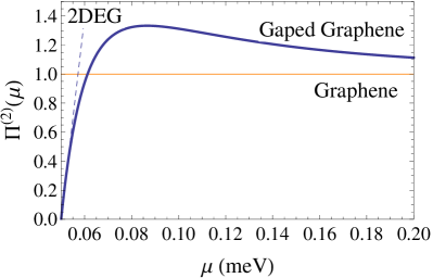
Figure 6: (Color online) The 2DEG polarization (in units of $\Pi^{(2)}(E_{g}=0)$ as a function of electro-chemical potential for chosen $E_{g}=11.6\;meV$

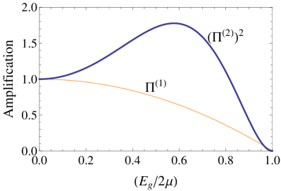
Figure 7: (Color online) Plots of the polarization functions in (17) and (18) with $E_{g}/2\mu$ in units of their value for $E_{g}=0$

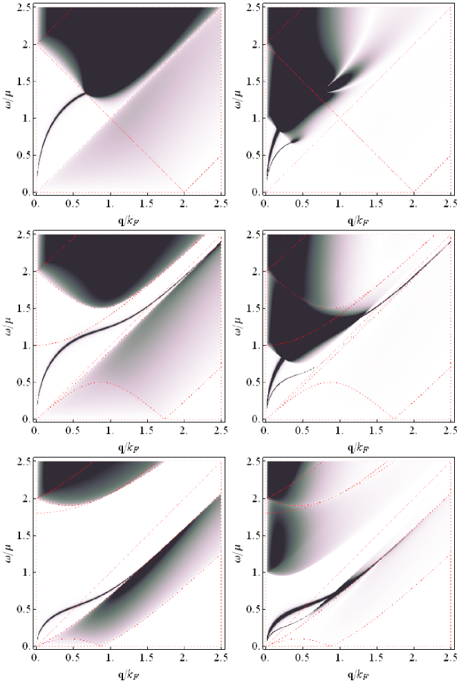
Figure 8: (Color online) Poles of the imaginary part of the spectral function. The left/right panels are density plots for linear absorption/SHG, respectively. For concreteness, the plasmon dephasing is chosen as $\gamma/2\mu=0.01.$

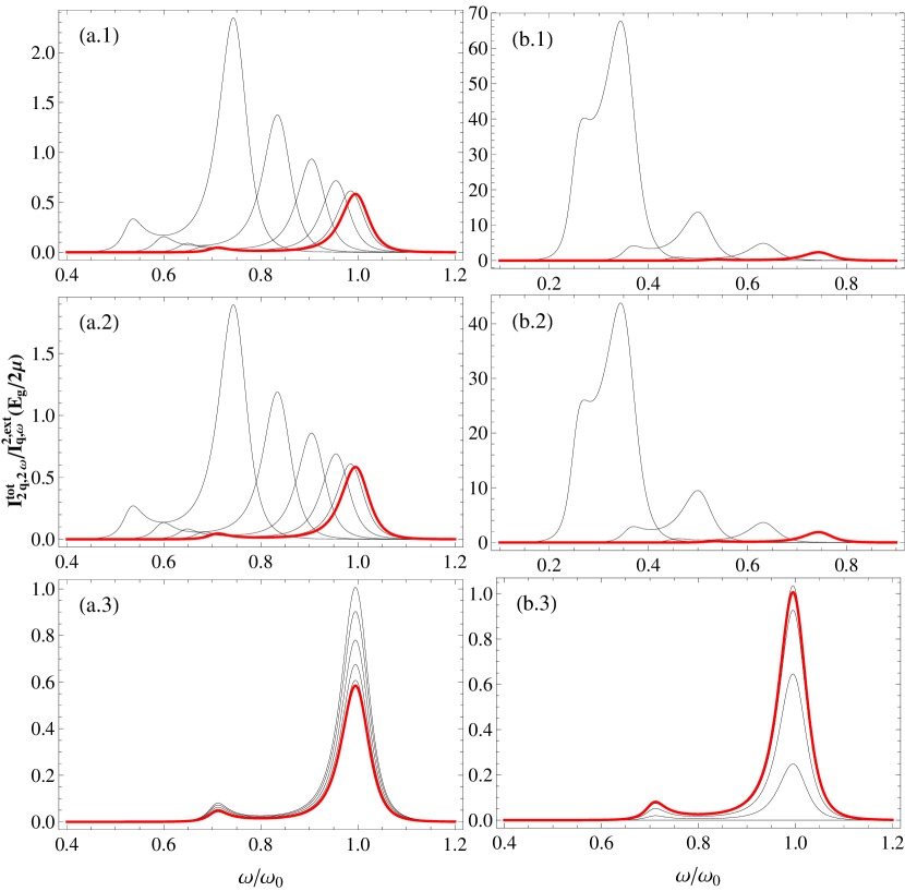
Figure 9: (Color online) Left panels show an increase starting with $E_{g}/2\mu=0.0$ (red curve), then $E_{g}/2\mu=0.1,\cdots.,0.5$. Right panels show growth for $E_{g}/2\mu=0.5$ (red curve), and $E_{g}/2\mu=0.6,\cdots,0.9$. Panels 2 are the effect due to change in $\omega_{p}$ only, The plasmon dephasing is set at $\gamma/2\mu=0.1$.

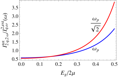
Figure 10: (Color online) Variation of the SHG signal along $\omega_{p}$ and $\omega_{p}/\sqrt{2}$. The latter was scaled up by a factor of twelve, for convenience.

IV Numerical Results and Discussion

We now complement our formalism by numerical simulations. For concreteness, we assume that the wavelength of incoming light to be $\lambda=800\;nm$ and the angle of incidence measured from the normal to the surface is $45^{\circ}$, as shown schematically in Fig. 2. The chemical potential is fixed by choosing $q/k_{F}=0.1$, thereby making $k_{F}=8.83\times 10^{6}\;m^{-1}$, i.e., $\mu=5.8\;meV$. This value of the chemical potential is well within the Dirac cone approximation. Consequently, we have $\omega_{p}(E_{g}=0)=\omega_{0}=1.54\;meV$, and $\omega_{0}/\sqrt{2}=1.09\;meV$. Those values are much smaller than the incoming light energy of $1.55\;eV$. This indicates that graphene is mostly transparent to light and only a small portion of it is specularly reflected even in the linear regime. The gap-inducing substrate is taken to be boron-nitride (BN) with background dielectric constant $\epsilon_{\infty}=7.1$. The nitrogen atoms of the substrate are in the center of the carbon-formed hexagons. In Ref. giovannetti , it was shown that the induced gap depends inversely on the distance $d$ from the graphene layer so that $d=3.65\;\AA$ corresponds to $E_{g}/2\mu=1$.

Some useful information regarding the SHG signal may be directly extracted from the poles of the spectral function in Eqs. (22) and (26) without employing the long wavelength approximation. In the left-hand column of Fig. 8, the linear response of gapped graphene is presented. Clearly, there is cross-over from Dirac ($E_{g}/2\mu=0$) to 2DEG-like ($E_{g}/2\mu=0.9$) plasmon behavior. The SHG possess poles as shown in the right-hand panel of Fig. 8. Of the two plasmon branches, the one at $\omega_{p}(q)$ is suppressed by linear response, whereas the one at $\omega_{p}(q)/\sqrt{2}$ may be spectrally resolved. However, when $E_{g}/2\mu=0$, both branches are Landau damped when $\omega/\mu>1-q/k_{F}$. Once the gap is increased to $E_{g}/2\mu=0.5$, the lower branch may appear in a region which opens up within the electron-hole continuum and is undamped beyond the long wavelength limit. For larger values of the gap, both branches merge with the electron-hole continuum at the same value of $q/k_{F}$. As the gap is further increased, both plasmon frequencies are reduced in accordance with the reduction in the linear response polarization function, as indicated in the right panel of Fig.6. Consequently, the spectral separation between them gets reduced, thereby making it more difficult to detect the lower SHG branch.

In order to study relative intensities of these plasmon branches, we must resort to the full version of the intensity ratio given in Eq. (29), thereby limiting ourselves to the long wavelength regime. One of the main factors determining that ratio is the square of the second-order polarization shown in Fig. 6. When $E_{g}/2\mu=0.6$, the second -order polarization reaches its maximum value which is seventy times larger than that of gapless graphene. To explain the maximum, it is convenient to fix the value of the gap at $E_{g}=11.6\;meV$ and then vary the chemical potential as shown in the left panel of Fig. 6. For small values of the chemical potential we have 2DEG-like behavior with the second-order polarization $\sim\mu$. For its large values, we have Dirac-like behavior with the second order polarization being independent of the chemical potential. Therefore, the maximum is the cross-over point between those two regimes.

The experimentally measurable Eq.(29) before and after cross-over is shown in panels (a) and (b) of Fig. 9. As we mentioned above, there are two factors affecting SHG intensity: the second-order polarization, given by the numerator, and the change in the plasmon frequency, given by the denominator, in Eq.(29)). Their separate effects are shown in panels (2) and (3) of Fig. 9. Those two effects work in favor of each other before the cross-over and against each other after that. Nevertheless, we observe steady growth of SHG intensity with $E_{g}$, making it an order of magnitude larger than that of conventional graphene. Fig.10 demonstrates that the lower $\omega_{p}/\sqrt{2}$ plasmon branch continues to grow with increased $E_{g}/2\mu$. This opens up an experimental avenue to identify those branches without relying on their spectral separation. This is similar to the effect of DC current on SHG but without underlying anisotropy induced by the currentbykov .

V Concluding Remarks

We have investigated the influence of substrate-induced gap in graphene on SHG signal. The maximum of the signal was attributed to an additional plasmon branch at $\omega_{p}/\sqrt{2}$. A red shift and an order of magnitude enhancement of that resonance with increased gap or reduced electro-chemical potential was demonstrated. The intensity of that branch increases more rapidly than the conventional $\omega_{p}$ branch which compensates for their reduced spectral separation. Our formalism is an alternative to DC induced enhancement in SHG but without accompanying the latter anisotropy in SHG signal.

References

(1) For a review, see R. W. Boyd, Nonlinear Optics
(Academic Press, New York, 1992).
(2) S. Mukamel, ”Principles of Nonlinear Optics”, Oxford University Press, 1999.
(3) E.H. Hwang, S. Das SArma, Phys. Rev. B, 75, 205418, (2007).
(4) P.K. Pyatkovskiy, J. Phys.:Condens. Matter, 21, 025506, (2009).
(5) T. Park, Godfrey Gumbs, and Y.C. Chen: Properties of
the second-order nonlinear optical susceptibility in
Asymmetric Undoped-AlGaAs/InGaAs Double Quantum Wells, Journal of
Applied Physics: 86, 1467-1470 (1999).
(6) J. Khurgin, Appl. Phys. Lett. 51, 2100 (1987).
(7) O. Vafek, Phys. Rev. Lett.,97, 266406, (2006).
(9) G. Giovannetti, P.A. Khomyakov, G. Brocks, P.J. Kelly, J. Brink, Phys. Rev. B.,
76 073103, (2007).
(10) E. Rosencher, P. Bois, J. Nagle, E. Costard,
and S. Delaite, Appl. Phys. Lett. 55, 1597 (1989).
(11) S. J. B. Yoo, M. M. Fejer, R. L. Byer, and J. S. Harris
Jr., Appl. Phys. Lett. 58, 1724 (1991).
(12) P. J. Harshman and S. Wang, Appl. Phys. Lett.
60, 1277 (1992).
(13) M. J. Shaw, K. B. Wong, and M. Jaros, Phys. Rev. B
48, 2001 (1993).
(14) M. Seto at. al., Appl. Phys. Lett. 65, 2969 (1994).
(15) Y. M. Cai, S. Yamada, O. Zamani-Khamiri, and A. P.
Garito, and K. Y. Wong, Phys. Rev. B 55, 12 985 (1997).
(16) H. Kuwatsuka and H. Ishikawa, Phys. Rev. B
50, 5323 (1994).
(17) L. Tsang, D. Ahn, and S. L. Chuang, Appl. Phys. Lett.
52, 697 (1988).
(18) M. M. Fejer, S. J. B. Yoo, R. L. Byer, A. Harwitt,
and J. S. Harris Jr., Phys. Rev. Lett. 62, 1041 (1989).
(19) L. C. West and S. J. Eglash, Appl. Phys. Lett.
46, 1156 (1985).
(20) R. Enderlein and N. J. M. Horing, Fundamentals of
Semiconductor Physics and Devices (World Scientific, Singapore, 1997)
Sec. 3.7.
(21) For InxGa1-xAs, the energy gap (in eV) is
; for AlxGa1-xAs, the energy gap (in eV) is
. The band offset for the conduction band is taken to
be and
for the valence band, where is the discontinuity
of the
energy gap for the two bulk materials forming the adjacent layers.
(22) L. Lang and K. Nish, Appl. Phys. Lett. 45,
98 (1984).