Near-Limb Zeeman and Hanle Diagnostics

Abstract

“Weak” magnetic-field diagnostics in faint objects near the bright solar disk are discussed in terms of the level of non-object signatures, in particular, on the stray light in telescopes. Calculated dependencies of the stray light caused by diffraction at the 0.5, 1.6, and 4 meter entrance aperture are presented. The requirements for micro-roughness of refractive and reflective primary optics are compared. Several methods for reducing the stray light (the Lyot coronagraphic technique, multiple stages of apodizing in the focal and exit pupil planes, apodizing in the entrance aperture plane with a special mask) and reducing the random and systematic errors are noted. An acceptable level of stray light in telescopes is estimated for the $V$-profile recording with a signal-to-noise ratio greater than three. Prospects for the limb chromosphere magnetic measurements are indicated.

1 Introduction

S-Introduction Near-limb Zeeman and Hanle diagnostics are connected with weak magnetic-field measurements in the upper solar atmosphere: prominences, the chromosphere, and the corona. Key items of magnetic measurements in the upper solar atmosphere are low-scattered-light feed optics (telescopes), an advanced analyzing equipment (polarimeters), and advanced recording equipment. So far, such measurements have not become routine in spite of available advanced coronagraphs, polarimeters, and recording systems [Lin, Kuhn, and Coulter (2004), Tomczyk et al. (2008)]. This is a task for forthcoming exciting ground- and space-based projects [Keil et al. (2003), Rimmele et al. (2010), Wagner et al. (2010), Tomczyk (2011), Peter et al. (2012)]. Non-solar object signatures in the final focal plane, in particular, the stray light [$I_{\rm stray}$], the sky brightness [$I_{\rm sky}$], and the continuum corona [$I_{\rm cont}$] complicate both linear and circular non-eclipse coronagraphic and eclipse polarimetry.

In this article we consider general expressions applicable in the upper solar atmosphere and several previous long-term magnetic measurements in prominences with the emphasis on $I_{\rm stray}$ of feeding optics (Section 1), dependencies of $I_{\rm stray}$ on distance caused by diffraction at the edge of an entrance aperture of 0.5, 1.6, and 4.0 meters and several ways of reducing $I_{\rm stray}$ (Section 2), reducing random and systematic errors (Section 3) and acceptable level of $I_{\rm stray}$ for the $V$-profile recording with a signal-to-noise ratio $>$ three (Section 4). Finally, prospects for magnetic measurements in the upper solar atmosphere are noted.

1.1 General Expressions

The term “weak magnetic field” is used when the Zeeman splitting [$\delta\lambda_{B}$] is three – four orders of magnitude less than the line width [$\Delta\lambda$]: the full width at half maximum]. $\delta\lambda_{B}=4.67\times 10^{-13}g\lambda_{0}^{2}B_{\prime\prime}$, where $\lambda_{0}$ is the wavelength in Å, $B_{\prime\prime}$ denotes the strength of longitudinal magnetic field in G, and $g$ is the Landé factor. As a rule, the effective Landé factor [$g_{e}$] is used to take into account the different contributions to the magnetic splitting caused by different components of the line. The left part of Figure 1 shows $\delta\lambda_{B}$ versus $B_{\prime\prime}$ for the chromospheric He I D3 ($g_{e}=1.12$) and 1083.0 nm ($g_{e}=1.46$), H I H$\alpha$ ($g_{e}=1.05$), and coronal Fe XIII 1074.7 nm ($g_{e}=1.46$) lines. The $g_{e}$ used for the He I lines does not take into account the low-intensity component, that is valid when $\Delta\lambda_{D3}\geq 0.4$ Å and $\Delta\lambda_{1083}\geq 1$ Å. $\delta\lambda_{B}$ of the IR lines differ by a factor of $0.99$ and are presented by the same curve. The $\delta\lambda_{B}$ range is $2\times(10^{-4}$ – $10^{-3})$ for $B_{\prime\prime}=10-20$ G.

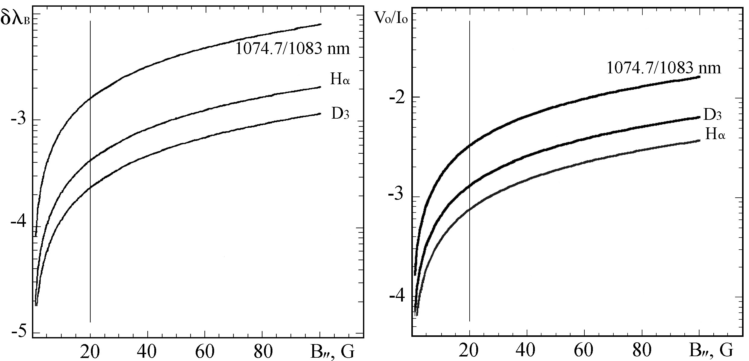
Figure 1.: The Zeeman splitting [$\delta\lambda_{B_{\prime\prime}}$] (left) and $k-$factor [$V_{0}/I_{0}$] (right) versus longitudinal magnetic-field strength [$B_{\prime\prime}$] for H I H$\alpha$, He I D₃, and 1083.0 nm, and Fe XIII 1074.7 nm lines.Fig1

In prominences, the chromosphere, and the corona $\Delta\lambda=0.4$ – 1 Å, and in the first approximation the upper part of $I$-profiles is well fitted by a gaussian. In “weak” fields the $V$-profile is proportional to the first derivative of the $I$ one.

$$V(\lambda)\approx\mathrm{dI}=-I_{0}\frac{2(\lambda-\lambda_{0})\times\mathrm{d}\lambda}{\Delta\lambda_{D}^{2}}\exp^{-\left(\frac{\lambda-\lambda_{0}}{\Delta\lambda_{D}}\right)^{2}},$$ (1)

where $I_{0}$ is the peak of the line intensity, $\lambda_{0}$ denotes the wavelength of the emission line, $\lambda$ is measured from $\lambda_{0}$, and $\Delta\lambda_{D}$ is the Doppler width. Equating the first derivative of $V$ to zero, we find the value of the $V$ peak [$V_{0}$] and the wavelength corresponding to $V_{0}$ [$\lambda_{B}$] as follows:

$$V_{0}\approx I_{0}\frac{\Delta\lambda_{D}\exp^{-\left(\frac{\Delta\lambda}{\sqrt{2}\Delta\lambda_{D}}\right)^{2}}}{\sqrt{2}\Delta\lambda_{D}^{2}}\delta\lambda_{B}\approx 1.4\times I_{0}\frac{\delta\lambda_{B}}{\Delta\lambda};\quad\lambda_{B}=\lambda_{0}\pm\frac{\Delta\lambda_{D}}{\sqrt{2}}\approx\pm 0.71\Delta\lambda_{D}.$$ (2)

Let us introduce a $k$-factor that is defined as the ratio of $V_{0}$ to $I_{0}$ and is needed for further estimates. In other words, $k$ indicates the amplification factor in the $V$ channel to record $I$ and $V$ on the same scale.

$$k=\frac{V_{0}}{I_{0}}\approx 1.4\times\frac{\delta\lambda_{B}}{\Delta\lambda}.$$ (3)

$k$($B_{\prime\prime}$) is shown in Figure 1 (right). Sophisticated polarimeters were needed to record the $V$-profile which is $7\times 10^{-4}I$ when using H$\alpha$ line and $B_{\prime\prime}=20$ G.

1.2 Feeding Optics of Previous Long-term Prominence Magnetic-Field Measurements

The direct magnetic-field determination in the upper solar atmosphere is based on the circular and linear-polarization analysis. The Zeeman analysis does not need any assumption on the mechanism of radiation and allows an approach close to the limb. The main steps of several long-term magnetic studies in prominences are outlined in the recent memoir by tandberg:2011. The feeding optics used (telescopes with the entrance aperture $<0.5$ m) are briefly noted below. Hereinafter, only references concerning the aspects of $I_{\rm stray}$ are cited.

1. The first magnetic measurements in active prominences were made by zirin:1961 and ioshpa:1962: Babcock-type type magnetographs, 30-cm solar tower telescopes, B${}_{\prime\prime}\approx 100$ G.

2. Next successes were based on magnetographs developed specifically for Zeeman analysis in prominences [Lee, Rust, and Zirin (1965), Lee, Harvey, and Tandberg-Hanssen (1969)] and Climax 40-cm coronagraph: the magnetograph slit of [$14-25^{\prime\prime}$]; an integration time up to 10 minutes. rust:1966 carried out magnetic research in quiescent prominences (QP): $B_{\prime\prime}$ ranges from a few G to 10 G, sometimes $20-30$ G. harvey:1968, malville:1968, and harvey:1969 carried out measurements in active prominences (AP): $B_{\prime\prime}=40-200$ G, possible dependence on the phase of solar cycle, the angle between the field vector and the long axis of prominences [$\alpha]<20^{\circ}$ [Tandberg-Hanssen and Anzer (1970)].

   Determinations of the magnetic-field vector in prominences have been made by athay:1983 with the advanced Stokes polarimeter and the 40-cm coronagraph of the Sacramento Peak Observatory: the polarimeter slit of $[7^{\prime\prime}\times 10^{\prime\prime}]$, an integration time of two minutes.

3. Contradictory results were reported by smolkov:1971 and bashkirtsev:1971 for the first stage of their measurements with the 50-cm horizontal solar telescope and the magnetograph scanning across the line profile: the magnetograph slit of $7^{\prime\prime}$, $B_{\prime\prime}$ up to 100 G in QP and up to 1000 G in AP.

4. The next long-term Zeeman analysis was made with Nikolsky’s magnetograph developed in cooperation with Institute d’Astrophysique de Paris [En den, Kim, and Nikolskii (1977), Nikolskii, Kim, and Koutchmy (1982), Stepanov (1989)] and the 50-cm domeless refractive coronagraph: the magnetograph pinhole of $8^{\prime\prime}$, an integration time of 30 seconds.

   – A piezo-scanning Fabry–Perot interferometer with a pre-filter.

   – A LiNbO₃ crystal as an analyzer.

   – Measurements in the vicinity of the optical axis ($<30^{\prime\prime}$).

   – The use of the magnetic-field etalon [Kim (2000)].

   – Compensation of the instrumental polarization [Klepikov (1999)].

   Results of the statistical analysis were as follows [Kim (1990)]: $B_{\prime\prime}$ in QP of several G, sometimes reaching $30-40$ G; in AP $B_{\prime\prime}=40-150$ G; $\alpha\leq 25^{\circ}$; both the inverse and normal polarities may exist in the same prominence.

To summarize, only coronagraphs as feeding optics provided long-term “weak” magnetic-field measurements [10 – 20 G] in prominences.

1.3 Non-object Signatures

On average, $V_{0}$ depends on $I_{0}$, $\lambda$, $g$, and $B_{\prime\prime}$. Nevertheless, the Zeeman diagnostics in spicules are technically more complicated task despite the fact that their intensities are greater than the intensity of bright prominences. Significant noise appears when approaching the limb.

Non-object signatures complicate the direct near-limb Zeeman diagnostics. Let $S/N$ be the signal-to-noise ratio. In our case $S=V_{0}$ and $N$ is the noise in the $V$ channel caused mainly by input of non-object signatures: $I_{\rm stray}$, $I_{\rm cont}$, and $I_{\rm sky}$ that are one – three orders of magnitude lower than $I$. Photon noise is assumed. In the first approximation, $N\approx k\times\left[\sqrt{I_{\rm stray}}+\sqrt{I_{\rm sky}}+\sqrt{I_{\rm cont}}\right]$. Let $S/N=V_{0}/N$ be $\geq 3$. Using the expressions (2) and (3) we obtain

$$N\leq 0.47\times I_{0}\frac{\delta\lambda_{B}}{\Delta\lambda}\quad\Longrightarrow\quad\left[\sqrt{I_{\rm stray}}+\sqrt{I_{\rm sky}}+\sqrt{I_{\rm cont}}\right]\leq 0.47\frac{I_{0}\times\delta\lambda_{B}}{k\times\Delta\lambda}.$$ (4)

Note that for reasonable non-object signatures (the total $<10^{-5}$), $B_{\prime\prime}=20$ G, $\delta\lambda_{B}$ and $k$ derived from Figure 1, the above expression is satisfied for $I_{0}>7\times 10^{-3}$ in H$\alpha$ and $>10^{-2}$ in IR lines that correspond to prominences. The intensity of coronal lines is much lower. An increase of the integration time and the entrance aperture is required to effectively increase the incoming flux.

2 Reducing the Stray Light in Telescopes

The existence of large-spread-angle stray light may significantly affect polarization measurements. According to chae:1998, the observed polarization degrees are always underestimated. The main sources of “parasitic” background in the final focal plane of any telescope are the following:

1. A ghost solar image produced by multiple reflections in the primary lens.

2. Random inhomogeneities in the glass of the primary lens.

3. Departures of the surface of the primary optics from a uniform shape.

4. Diffraction of the solar disk light at the entrance aperture [$I_{\rm dif}]$.

5. Scattering at micro-roughness of the primary optics [$I_{\rm sc}$].

6. The sky brightness [$I_{\rm sky}$].

7. The continuum corona [$I_{\rm cont}$].

8. The dust on the primary optics [$I_{\rm dust}$].

Reducing items i) –iv) was partly discussed by newkirk:1963. Items iv) –vi) are negligible during total solar eclipse (TSE), and they dominate for high-altitude coronagraphic observations. Reducing the item viii) for 53-cm refractive primary optics (our experience) was made by cleaning the lens before each set of observations. But this item becomes very important for large-aperture reflective primary optics. Below the role of the stray light for magnetic-field measurements will be discussed. Hereinafter we denote $I_{\rm stray}$ as $I_{\rm dif}+I_{\rm sc}$.

2.1 Reducing the Stray Light Caused by Diffraction of the Bright Round Source at the Round Aperture

The diffraction of the bright round source at the round aperture was treated by nagaoka:1920. For estimations of $I_{\rm dif}$, we used the simplified expression suggested by sazanov:1968 which is valid in the range R $<1.3$ R_⊙. Deviations not more than $20\,\%$ are expected as compared with values based on Nagaoka’s equations.

$$\log{I_{\rm dif}(\rho)}=\log\frac{2\lambda}{\pi^{3}D\gamma_{0}}+\log\left(\frac{\sqrt{1+(\nu-1)^{2}}}{\nu-1}-\frac{\sqrt{1+(\nu+1)^{2}}}{\nu+1}\right)-0.27(\nu-1)-0.017,$$ (5)

where $\rho$ is the distance from the solar disk center in the units of R_⊙, $\nu=\frac{\rho}{a}$, $a=\frac{\pi D}{\lambda}\gamma_{0}$ is the radius of the round source in arbitrary units, $D$ is the diameter of the primary lens, $\gamma_{0}$ is the angular radius of the source. $I_{\rm dif}$(R) is shown in Figure 2 for H$\alpha$ (left) and near IR (right) lines for 0.5 m, 1.6 and 4 m apertures. Vertical lines indicate typical maximum altitudes observed [$h$] of QP ($40^{\prime\prime}\approx 0.042$ R_⊙), active region filaments (ARF) ($25^{\prime\prime}\approx 0.026$ R_⊙), and the upper chromosphere ($4^{\prime\prime}\approx 0.004$ R_⊙). Hereinafter intensities, brightness, equivalent width are given in units of the 1 Å nearby solar-disk continuum.

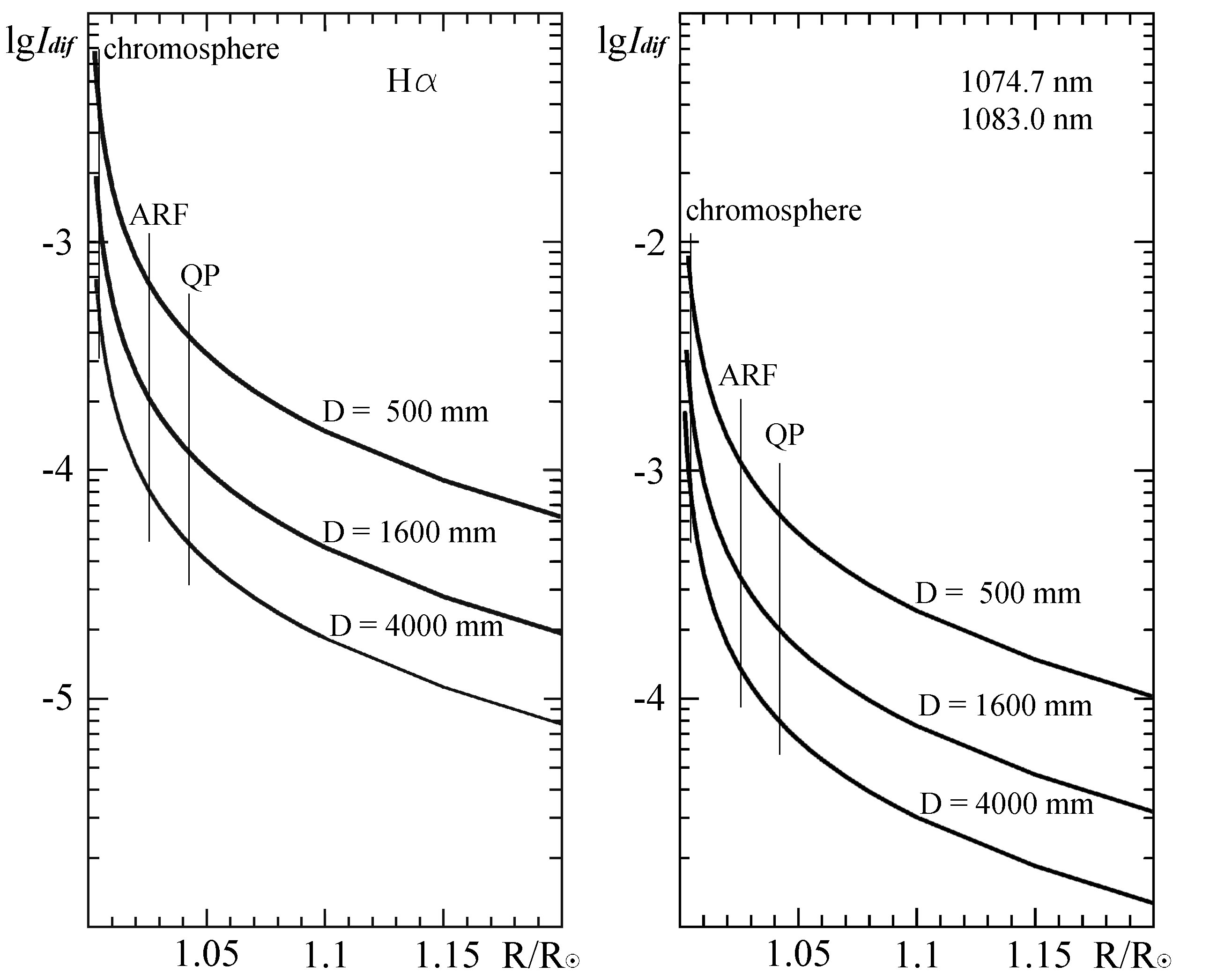
Figure 2.: Stray light caused by diffraction of the solar disk light at the entrance aperture. Left: H$\alpha$ line. Right: the He I 1083.0 nm and Fe XIII 1074.7 nm lines.Fig2

It is seen that the stray light in H$\alpha$ caused by diffraction at the 0.5 m aperture of a conventional (non-coronagraphic) telescope can reach $10^{-3}$ at prominence heights and is $>5\times 10^{-3}$ at the chromosphere level.

2.1.1 Coronagraphic Technique (the Lyot Method)

The coronagraphic technique suggested by lyot:1931 is based on the masking in the primary focal plane and in the plane of the exit pupil to eliminate i) and ii), and to minimize the input of iv). The optical sketch of the Lyot-type coronagraph has the primary single lens, the primary focal plane, the mask in the primary focal plane (an artificial Moon), the field lens, the mask in the plane of the exit pupil (the Lyot stop), the relay optics, and the final focal plane. Multiple Fresnel reflections at the surfaces of the primary lens create a system of the solar-disk images, decreasing in brightness. For a single primary lens with the refraction index $n=1.5$, the brightness ratio of the first, most bright reflection to the the solar disk one is $(n-1)^{4}/(n+1)^{4}=1/625$, and the ratio of the primary focal length to the space between the image and the lens is $[2/(n-1)]+3=7$. A round screen in the center of the Lyot stop results in removal of the reflection. The procedure is not applicable for the multi-lens primary optics, as the brightest reflection is near the primary focal plane. The correct use of the Lyot method results in $I_{\rm dif}$ reducing in one to two orders of magnitude depending on the size of the mask in the primary focal plane and in the plane of the Lyot stop. In practice, reducing $I_{\rm stray}$ by $\approx 50-100$ (the coronagraphic efficiency [$K$]) for prominences and 10 – 25 for the chromosphere can be achieved depending on the height observed.

2.1.2 Multiple Cascade Coronagraphic Technique

To our knowledge, the multiple-cascade coronagraphic technique has not been used practically. terrile:1989 found that an additional factor of more than ten can be achieved through multiple stages of apodizing in both the focal plane and in the Lyot-stop plane. The calculated point spread function (PSF) showed that in such a hybrid coronagraph $I_{\rm dif}$ can be reduced by more than three orders of magnitude.

We used the two stage coronagraphic approach for the last version of Nikolsky’s magnetograph [Stepanov (1989)]. The main goal was to match the focal ratio of the coronagraph with the spectral resolution of the Fabry–Perot interferometer through the inclusion of an additional focal and the Lyot-stop planes. This complicated the optical adjustment of the “coronagraph + magnetograph” assembly. Depending on the brightness of prominences, the magnetic-field strength, and the height observed, the signal-to-noise ratio became two – three times better.

2.1.3 Apodizing with a Special Mask in the Plane of an Entrance Aperture

The diffraction pattern in the focal plane is the result of discontinuity of the transmission function [$G$] (or its derivatives) of the entrance aperture. The characteristic frequency of the damping intensity oscillations depends on the distance between the points of discontinuity, the asymptotic damping rate depends on the order of the derivative in which the continuity of $G$ ($G^{2}$ in intensity) is broken. For a round aperture, there is a discontinuity in the zero derivative: $G(\rho)=1$ in the range $\rho<1$ and $G=0$ in the range $\rho\geq 1$, where $\rho$ is the distance from the center of aperture. In the case of a point source, it creates the Airy diffraction pattern $I\propto[J_{1}(r)/r]^{2}$ with intensity damping as $r^{-3}$, where $J_{1}(x)$ is the Bessel function of the first kind. A mask with variable transmission [$G(\rho)=1-\rho^{2}$] has discontinuities only in the first derivative. The use of such a mask in the plane of the entrance aperture results in the diffraction image $I\propto{\{[J_{1}(r)+J_{3}(r)]/r\}}^{2}$ with the more effective damping as $r^{-5}$.

We considered an extended object, e.g., the Sun [Kim et al. (1995)] using Nagaoka’s equations [Nagaoka (1920)]. The stray light in the center of the solar disk image caused by diffraction at the entrance aperture is given by

$$I_{\rm dif}(0)=1-J_{0}^{2}(a)-J_{1}^{2}(a),$$ (6)

where $a=(\pi D\sin{\gamma_{0}})/\lambda,\lambda$ is the wavelength, $\gamma_{0}$ is the angular radius of solar disk, and $D$ is the diameter of aperture. If $a\gg 1$, then $I_{\rm dif}(0)\approx 1-2/(\pi a)$. For $\gamma_{0}=960^{\prime\prime}$, $\lambda=600$ nm, $D=200$ mm, we obtain $a=4874$ and $I_{\rm dif}(0)=(1-1.3)\times 10^{-4}$.

In the case when the entrance aperture is apodized by the mask $G=(1-\rho^{2})$, we found the relation between the apodized [$I^{a}_{\rm dif}$] and non-apodized [$I_{\rm dif}$] for points at the angular distance $\gamma=(1+\epsilon)\gamma_{0}$ from the disk center:

$$I^{a}_{\rm dif}(\epsilon)\simeq 2/3\pi^{4}{[I_{\rm dif}(\epsilon)]}^{3}.$$ (7)

Let us estimate the efficiency of the mask for chromospheric and prominence heights and $a\approx 5000$.

• The upper chromosphere heights: $h=4^{\prime\prime}$, $\epsilon=0.004$ $(\epsilon\gamma_{0}=4^{\prime\prime})$. Then $I(0.004)=10^{-2}$ and $I^{a}(0.004)=0.7\times 10^{-4}$. Calculated efficiency up to $10^{2}$ can be achieved.

• Quiescent prominence heights: $h=40^{\prime\prime}$, $\epsilon=0.04$ ($\epsilon\gamma_{0}=40^{\prime\prime})$. Then $I_{\rm dif}(0.04)=10^{-3}$ and $I^{(a)}_{\rm dif}(0.04)=0.7\times 10^{-7}$. Calculated efficiency up to $10^{4}$ can be achieved.

No classical Lyot-type coronagraphs are needed. Note that the mask $(1-\rho^{2})$ reduces transmittance by a factor of three.

2.2 Comments on Scattering by Micro-Roughness of the Primary Optics

In this subsection, we do not analyze scattering by micro-roughness of the primary optics. This is a topic requiring detailed studies. In the case of the statistical nature of the micro-roughness, $I_{\rm sc}$ is proportional to the square of the average height of the inhomogeneity (RMS). The fabrication of super-smooth primary optics is the key technology for creating a low-scattered-light coronagraph. Reflecting optics are achromatic and do not depend on bulk inhomogeneities of the material compared to a refractor. Let $n$ be the index of refraction. At the same value of RMS, the energy scattered by a reflecting surface ($n^{*}=-1$) [$I_{\rm sc}$] is greater by a factor of $[(n^{*}-1)/(n-1)]^{2}=16$ compared to the refractive case. Possible ways to reduce the scattered light include the following.

• The use of a super-smooth primary optics with RMS = 3 – 10 Å. Pioneering studies performed by socker:1988 showed that the $I_{\rm stray}$ of a 9.8 cm diameter super-smooth silicon mirror is comparable with the stray light of a single lens.

• The use of moderately smooth primary optics with a given profile of the micro-relief can significantly reduce the scattered light in the range of interest. According to numerical calculations by romanov:1991 made for the Earth-environment monitoring, RMS of 25 Å and the spatial period of the micro-relief (the correlation length of inhomogeneities) of $0.76-0.78$ $\mu$ can provide scattered light of $\approx 10^{-5}$ in the range $<1.1$ R_⊕ where R_⊕ is the radius of the Earth.

3 Acceptable Level of the Stray Light in Telescopes for Zeeman Diagnostics

Using Equation (4), Figures 1 and 2, let us estimate the acceptable level of the stray light in telescopes for Zeeman diagnostics with the signal-to-noise-ratio $\geq 3$. Several conditions exist.

• The stray light is caused by diffraction at the entrance aperture (a super-smooth primary optics).

• The noise of the recording assembly is negligible.

• $W$ is the equivalent width of the emission line.

• The instrumental width is $0.7\Delta\lambda_{D}$ $\approx 0.5\Delta\lambda$ to achieve the maximum signal-to-noise ratio [Nikolskij et al. (1985)].

• In the case of scattering by aerosols ($\sim\lambda^{-2}$), $I_{\rm sky}=10^{-5}$ in H$\alpha$ and $I_{\rm sky}\approx 2\times 10^{-6}$ in the IR lines.

• $I_{\rm cont}$ passed through the instrumental profile is $<10^{-6}$.

H$\alpha$ bright prominences, B${}_{\prime\prime}=100$ G: W $=10^{-1}$, $\Delta\lambda\approx 0.6$ Å. $I_{0}=5\times 10^{-2}$, $\delta\lambda_{B}=2\times 10^{-3}$ and $k=4\times 10^{-3}$ (Figure 1). The required $I_{\rm stray}$ should be $\leq 5\times 10^{-4}$. Referring to Figure 2 (left), we see that the aperture of 0.5 meter provides this level of scattered light at $h>35^{\prime\prime}$. The first magnetic measurements in prominences with 30 cm solar tower telescopes as feeding optics confirm this [Zirin and Severny (1961), Ioshpa (1962)].

A non-coronagraphic 4 meter telescope with a super-smooth primary optics can provide Zeeman diagnostics of 100 G field strengths in bright prominences from $h\geq 10^{\prime\prime}$ as well.

H$\alpha$ moderate brightness prominences, B${}_{\prime\prime}=20$ G: $W=2\times 10^{-2}$, $\Delta\lambda\approx 0.6$ Å. $I_{0}=10^{-2}$, $\delta\lambda_{B}=4\times 10^{-4}$ and $k=7\times 10^{-4}$ (Figure 1). The required $I_{\rm stray}$ should be $\leq 2\times 10^{-5}$. Only coronagraphs (at the limits of 0.5 meter, and reliably with 4 meter apertures) provide the required $I_{\rm stray}$ from heights $>20^{\prime\prime}$. Note the crucial role of the sky brightness, the polarimeter performance, and the integration time.

Limb chromosphere, He I 1083.0 nm, B${}_{\prime\prime}=20$ G: $W\approx 3\times 10^{-2}$, $\Delta\lambda\approx 0.8$ Å. $h=4^{\prime\prime}$, $I_{0}=1.5\times 10^{-2}$, $\delta\lambda_{B}=1.3\times 10^{-3}$ and $k=3\times 10^{-3}$ (Figure 1). Then the required $I_{\rm stray}\leq 1.6\times 10^{-5}$ will be provided with the 4 meter coronagraph in which the scattered light is reduced by $30-40$.

Corona, Fe XIII 1074.7 nm, B${}_{\prime\prime}=20$ G: $W=2\times 10^{-4},\Delta\lambda\approx 0.8$ Å. The expected total of all non-corona signatures is $\approx 10^{-5}$. $\delta\lambda_{B}=1.5\times 10^{-3}$, and $k=3.3\times 10^{-3}$ (Figure 1). $I_{0}=10^{-4}$, that is increasing $I_{0}$ up to $10^{2}$ (see above) is required. A 4 meter aperture allows an increase in the flux by 64 times as compared to a 0.5 meter one. In this case, the conditions will be similar to magnetic-fields measurements in moderate brightness prominences when using a 0.5 meter coronagraph. $I_{\rm sky}$, the performance of the polarimeter, and the integration time become important factors.

4 Reduction of Random and Systematic Errors

We have developed an approach for high-precision linear polarimetry with actual accuracy of $2\%$ for the linear polarization degree [$p$] and $2^{\circ}$ for the polarization angle [$\chi$] that allow us to obtain “polarization images” of an object: 2D distributions of $p$, $\chi$, and the sign of $\chi$. The description of the last version was presented recently [Kim et al. (2011)]. The key components are the following:

1. Low level of the sky brightness, $I_{\rm sky}$.

2. A low level of the stray light in telescopes, $I_{\rm stray}$.

3. Uniformity of the polarizer performance for any “point” of the image.

4. Reduction of random errors based on “statistics”: the use of 24 orientations of a polarizer instead of traditional three.

5. Reduction of systematic errors based on Stokes-vector presentation of the light and the solution of the over-determined system of 24 equations (the number of equations is greater than the the number of unknowns) by the least squares.

The role of the last two points is shown below. We use the total solar eclipse of 29 March 2006 observations, as $I_{\rm sky}$ and $I_{\rm stray}$ were negligible during totality. The approach was applied to the red polarization movie of the continuum corona to check the potential of our method, the reliability of the predicted accuracy, and the importance of items iv) and v) for the near-limb polarimetry. The red series of 24 sequential frames centered at 25 seconds before the third contact [T₃] was treated in 2 ways to search for evidence for H$\alpha$ prominences in polarization as our red filter transmitted H$\alpha$ line. Until now, measurements of linear polarization in low-brightness prominences [$I<10^{-2}$] are rarely carried out in spite of available advanced polarimeters. Figure 3 shows the 2D distribution of $p$ in the range $0-8\,\%$ for distances $<1.1$ R_⊙ above the SW limb. The left distribution is based on three orientations of a polarizer spaced by $120^{\circ}$ and exhibits a noise of $3-7\,\%$. The right one is based on 24 orientations of the same series for the same position angle range and clearly reveals the polarized feature at position angle $P=251^{\circ}$ with $p=3-7\,\%$. Position angles are measured counter-clockwise from the N Pole of the Sun. The solar and lunar limbs, the scales of heights and $p$, and the N direction are shown. The step of the $p$-scale is $2\,\%$. Synoptic data from the Pulkovo Observatory identify this $p$-feature with a low brightness H$\alpha$ prominence ($10^{-3}-10^{-2}$) at the same $P=251^{\circ}$. It is known that in the absence of longitudinal magnetic fields, the polarization degree in prominences increases from $3$ to $8\,\%$ with an increase in height from $10^{\prime\prime}$ to $96^{\prime\prime}$. The distribution agrees with the expected $p$-values and indirectly confirms the accuracy $<2\,\%$. We note that these “raw” 2D distributions were obtained only to test the ability of our method to distinguish the near-limb several-percent linear polarization and to verify the accuracy $<2\,\%$. Actual values of $p$ are expected to be $1-2\,\%$ lower as the transfer to intensities was based on a polynomial approximation of degree four over the wide range of densities from the background to prominences and no corrections for the red coronal continuum input was made. The corrected eclipse linear polarimetry in prominences as well as $p$, $\chi$, and the sign of $\chi$ images will be discussed in a separate article.

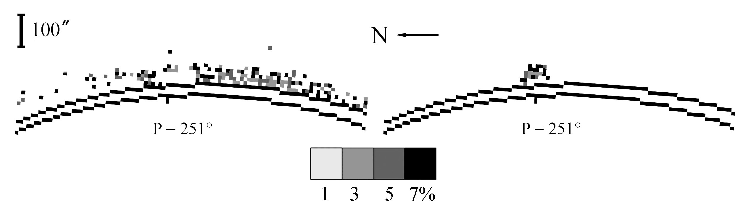
Figure 3.: The 2D distribution of $p$ in the red spectral interval including H$\alpha$ line based on three orientations of a polarizer (left) and on 24 orientations (right). The right $p$-image reveals the polarized feature at $P=251^{\circ}$, which is identified with the low-brightness H$\alpha$ prominence.Fig3

5 Summary

The stray light [$I_{\rm stray}$] seems to be a crucial factor determining the reliable near-limb $V$-profile recording in the range $<1.2$ R_⊙. Our estimates of non-object signatures quantitatively show that the most advanced polarimeter will be powerless if $I_{\rm stray}$ in a feeding optics exceeds the acceptable level. A brief comparison of several ways of $I_{\rm stray}$ reduction results in the following.

• The well-known coronagraphic technique (the Lyot method) provides the coronagraphic efficiency [$K$] of 10 – 100 depending on the size of mask in the primary focal plane and in the plane of the Lyot stop (depending on the object under study).

• According to our experience, multiple stages of apodizing in both the focal plane and in the Lyot-stop plane provides $K=2-3$ and complicates the optical adjustment of the “coronagraph + magnetograph” assembly.

• Apodizing with a mask with variable transmission placed in the plane of an entrance aperture [$G(\rho)=1-\rho^{2}$], where $\rho$ is the distance from the center of aperture. For a 200 mm aperture, the calculated efficiency factor up to $10^{2}$ at the upper chromosphere level [$4^{\prime\prime}$] and up to $10^{4}$ at the QP heights [$40^{\prime\prime}$] can be achieved. Recent technology advances allow the discussion on manufacturing such a mask. Synoptic chromospheric and prominence magnetic research seem to be reliable.

• The use of a super-smooth primary optic with RMS = 3 – 10 Å or a moderately smooth primary optics (RMS of 25 Å) with a given profile of the micro-relief can significantly reduce the scattered light in the range of interest.

• The important role of reduction of random and systematic errors is shown by the example of eclipse linear polarimetry of prominences.

Estimation of the acceptable level of the stray light in 0.5, 1.6, and 4 meter aperture telescope for Zeeman diagnostics with the signal-to-noise-ratio of $>3$ show that the 4 meter-aperture ATST with $I_{\rm stray}<10^{-5}$ will provide $V$-profile recording of “weak” fields [$B_{\prime\prime}=10-20$ G] in prominences in visual and IR lines, the limb chromosphere and corona in IR lines with the finest magnetic “resolution” comparable with the characteristic size of the structures.

Acknowledgements

This work was partially supported by research project No 11-02-00631 of Russian Foundation for Basic Research. We are very indebted to the referee for corrections and important comments concerning the sources of stray light.

References

- Athay et al. (1983) Athay, R.G., Querfeld, C.W., Smartt, R.N., Landi Degl’Innocenti, E., Bommier, V.: 1983, Vector magnetic fields in prominences. iii - hei d3 stokes profile analysis for quiescent and eruptive prominences. Solar Phys. 89, 3 – 30.
- Bashkirtsev, Smolkov, and Shmulevsky (1971) Bashkirtsev, V.S., Smolkov, G.Y., Shmulevsky, V.N.: 1971,. Iss. po geomagnet., aeronom. fizike Solntsa 20, 212.
- Chae et al. (1998) Chae, J., Yun, H.S., Sakurai, T., Ichimoto, K.: 1998, Stray-light effect on magnetograph observations. Solar Phys. 183, 229 – 244.
- En den, Kim, and Nikolskii (1977) En den, O., Kim, I.S., Nikolskii, G.M.: 1977, Measurement of the prominences magnetic field. Solar Phys. 52, 35 – 36.
- Harvey (1969) Harvey, J.W.: 1969, Magnetic fields associated with solar active-region prominences. PhD thesis, University of Colorado at Boulder.
- Harvey and Tandberg-Hanssen (1968) Harvey, J.W., Tandberg-Hanssen, E.: 1968, The magnetic field in some prominences measured with the he i, 5876 + line. Solar Phys. 3, 316 – 320.
- Ioshpa (1962) Ioshpa, B.A.: 1962,. Geomag. Aeron. 2, 149.
- Keil et al. (2003) Keil, S., Rimmele, T., Keller, C., The ATST Team: 2003, Design and development of the advanced technology solar telescope. Astronom. Nachr. 324, 303 – 304.
- Kim (1990) Kim, I.S.: 1990, Prominence magnetic field observations. In: Ruzdjak, V., Tandberg-Hanssen, E. (eds.) IAU Colloq. 117: Dynamics of Quiescent Prominences, Lecture Notes in Physics, Berlin Springer Verlag 363, 49 – 69.
- Kim (2000) Kim, I.S.: 2000, Observing the solar magnetic field. In: Zahn, J.P., Stavinschi, M. (eds.) NATO ASIC, Adv. Solar Res. Eclipses from Ground and from Space, Kluwer Academic Publisher 558, 67 – 83.
- Kim et al. (2011) Kim, I.S., Lisin, D.V., Popov, V.V., Popova, E.V.: 2011, Eclipse high-precision linear polarimetry of the inner white-light corona: Polarization degree. In: Kuhn , J.R., Harrington, D.M., Lin, H., Berdyugina, S.V., Trujillo-Bueno, J., Keil, S.L., Rimmele, T. (eds.) Astron. Soc. Pacific, CS 437, 181 – 188.
- Kim et al. (1995) Kim, I., Bugaenko, O., Bruevich, V., Evseev, O.: 1995, Problems of reflecting coronagraphs. Bull. of Russian Acad. Sciences 59, 153.
- Klepikov (1999) Klepikov, V.Y.: 1999, Magnitnye polya spokoinykh protuberantsev (magnetic fields of quiscent prominences). PhD thesis, IZMIRAN, Moscow.
- Lee, Harvey, and Tandberg-Hanssen (1969) Lee, R.H., Harvey, J.W., Tandberg-Hanssen, E.: 1969, The improved solar magnetograph of the high altitude observatory. Appl. Opt. 8, 2370.
- Lee, Rust, and Zirin (1965) Lee, R.H., Rust, D.M., Zirin, H.: 1965, The solar magnetograph of the high altitude observatory. Appl. Opt. 4, 1081.
- Lin, Kuhn, and Coulter (2004) Lin, H., Kuhn, J.R., Coulter, R.: 2004, Coronal magnetic field measurements. Astrophys. J. Lett. 613, L177 – L180.
- Lyot (1931) Lyot, B.: 1931, Photographie de la couronne solaire en dehors des eclipses. C.R. Acad. Sci. 193, 1169.
- Malville (1968) Malville, J.M.: 1968, Magnetic fields in two active prominences. Solar Phys. 5, 236 – 239.
- Nagaoka (1920) Nagaoka, H.: 1920, Diffraction of a telescopic objective in the case of a circular source of light. Astrophys. J. 51, 73.
- Newkirk and Bohlin (1963) Newkirk, G. Jr., Bohlin, D.: 1963, Reduction of scattered light in the coronagraph. Appl. Opt. 2, 131.
- Nikolskii, Kim, and Koutchmy (1982) Nikolskii, G.M., Kim, I.S., Koutchmy, S.: 1982, Measurements of the magnetic field in solar prominences with a spectrally scanning magnetograph. Solar Phys. 81, 81 – 89.
- Nikolskij et al. (1985) Nikolskij, G.M., Kim, I.S., Koutchmy, S., Stepanov, A.I.: 1985, Measurement of magnetic fields in solar prominences. Astronom. Zhur. 62, 1147 – 1153.
- Peter et al. (2012) Peter, H., Abbo, L., Andretta, V., Auchère, F., Bemporad, A., Berrilli, F., Bommier, V., Braukhane, A., Casini, R., Curdt, W., Davila, J., Dittus, H., Fineschi, S., Fludra, A., Gandorfer, A., Griffin, D., Inhester, B., Lagg, A., Degl’Innocenti, E.L., Maiwald, V., Sainz, R.M., Pillet, V.M., Matthews, S., Moses, D., Parenti, S., Pietarila, A., Quantius, D., Raouafi, N.E., Raymond, J., Rochus, P., Romberg, O., Schlotterer, M., Schühle, U., Solanki, S., Spadaro, D., Teriaca, L., Tomczyk, S., Bueno, J.T., Vial, J.C.: 2012, Solar magnetism eXplorer (SolmeX). Exploring the magnetic field in the upper atmosphere of our closest star. Exp. Astron. 33, 271 – 303.
- Rimmele et al. (2010) Rimmele, T.R., Wagner, J., Keil, S., Elmore, D., Hubbard, R., Hansen, E., Warner, M., Jeffers, P., Phelps, L., Marshall, H., Goodrich, B., Richards, K., Hegwer, S., Kneale, R., Ditsler, J.: 2010, The Advanced Technology Solar Telescope: beginning construction of the world’s largest solar telescope. In: Soc. of Photo-Opt. Instrumen. Eng., SPIE CS 7733, 77330G – 77330G17.
- Romanov et al. (1991) Romanov, A.D., Starichenkova, V.D., Fes’kov, A.I., Folomkin, I.P.: 1991,. J. Opt. Tech. (OMP in Russian, No 6), 11 – 14.
- Rust (1966) Rust, D.M.: 1966, Measurements of the magnetic fields in quiescent solar prominences. PhD thesis, University of Colorado at Boulder.
- Sazanov (1968) Sazanov, A.A.: 1968, Bol’shoi vnezatmenny koronagraph izmir–gao an sssr i ego issledovanie (the large non-eclipse coronagraph izmir–gao as of the ussr and its research). PhD thesis, IZMIRAN, Moscow.
- Smol’kov and Bashkirtsev (1971) Smol’kov, G.Y., Bashkirtsev, V.S.: 1971, On the precision of records of the magnetic field in quiet prominences using a magnetograph. Solnech. Dann. Bull. Akad. Nauk SSSR 1971, 99 – 105.
- Socker and Korendyke (1988) Socker, D., Korendyke, C.: 1988, Stray light measurements of reflecting coronagraph mirrors at lambda = 6328 Å. Bull. Am. Astron. Soc. 20, 990.
- Stepanov (1989) Stepanov, A.A.: 1989, Magnitograficheskie issledovaniya protuberanzev (magnetographic research of prominences). PhD thesis, IZMIRAN, Moscow.
- Tandberg-Hanssen (2011) Tandberg-Hanssen, E.: 2011, Solar prominences - an intriguing phenomenon. Solar Phys. 269, 237 – 251.
- Tandberg-Hanssen and Anzer (1970) Tandberg-Hanssen, E., Anzer, U.: 1970, The orientation of magnetic fields in quiescent prominences. Solar Phys. 15, 158 – 166.
- Terrile (1989) Terrile, R.J.: 1989, Direct imaging of extra-solar planetary systems with the Circumstellar Imaging Telescope (CIT). In: Weaver, H.A., Danly, L. (eds.) The Formation and Evolution of Planetary Systems, Space Telescope Science Institute Symposium Series 3, Cambridge University Press, University Printing House, 333 – 334.
- Tomczyk (2011) Tomczyk, S.: 2011, The Coronal Solar Magnetism Observatory (COSMO). AGU Fall Meeting Abstracts, B1952.
- Tomczyk et al. (2008) Tomczyk, S., Card, G.L., Darnell, T., Elmore, D.F., Lull, R., Nelson, P.G., Streander, K.V., Burkepile, J., Casini, R., Judge, P.G.: 2008, An instrument to measure coronal emission line polarization. Solar Phys. 247, 411 – 428.
- Wagner et al. (2010) Wagner, J., Hansen, E., Hubbard, R., Rimmele, T.R., Keil, S.: 2010, Advanced technology solar telescope project management. In: Soc. Photo-Opt. Instrumen. Eng. (SPIE), CS 7738, 77380Q – 77380Q24.
- Zirin and Severny (1961) Zirin, H., Severny, A.: 1961, Measurement of magnetic fields in solar prominences. Observ. 81, 155 – 156.