Adaptive Hierarchical Data Aggregation using Compressive Sensing (A-HDACS) for Non-smooth Data Field

Abstract

Compressive Sensing (CS) has been applied successfully in a wide variety of applications in recent years, including photography, shortwave infrared cameras, optical system research, facial recognition, MRI, etc. In wireless sensor networks (WSNs), significant research work has been pursued to investigate the use of CS to reduce the amount of data communicated, particularly in data aggregation applications and thereby improving energy efficiency. However, most of the previous work in WSN has used CS under the assumption that data field is smooth with negligible white Gaussian noise. In these schemes signal sparsity is estimated globally based on the entire data field, which is then used to determine the CS parameters. In more realistic scenarios, where data field may have regional fluctuations or it is piecewise smooth, existing CS based data aggregation schemes yield poor compression efficiency. In order to take full advantage of CS in WSNs, we propose an Adaptive Hierarchical Data Aggregation using Compressive Sensing (A-HDACS) scheme. The proposed schemes dynamically chooses sparsity values based on signal variations in local regions. We prove that A-HDACS enables more sensor nodes to employ CS compared to the schemes that do not adapt to the changing field. The simulation results also demonstrate the improvement in energy efficiency as well as accurate signal recovery.

I Introduction

Energy efficiency is a major target in the design of wireless sensor networks due to limited battery power of the sensor nodes. Also, at times it is difficult to replenish battery power depending on the application area. Since data communication is the most basic but high energy consuming task in sensor networks, a plethora of research work has been done to improve its energy consumption [1] [2] [3] [4]. Compressive Sensing (CS) [5] [6] has emerged as a promising technique to reduce the amount of data communicated in WSNs. It has been also applied in other application areas such as photography, shortwave infrared cameras, optical system research, facial recognition, MRI, etc. [7]. Luo et. al. [8] proposed the use of CS random measurements to replace raw data communication in data aggregation tasks in WSNs, thus reducing the amount of data transmitted. However, their technique introduced redundant data communication in nodes that were farther away from the root node of the data aggregation tree. Xiang et. al.[9] [10] optimized this scheme by reducing the data transmission redundancy. In our previous work, We further improved CS based data aggregation by proposing a Hierarchical Data Aggregation using Compressive Sensing (HDACS) [11] that introduced a hierarchy of clusters into CS data aggregation model and achieved significant energy efficiency.

However, most of the previous work has used CS under the assumption that data field is smooth with negligible white Gaussian noise. In these schemes, signal sparsity is calculated globally based on the entire data field. In more realistic scenarios, where data field may have regional fluctuations or it is piecewise smooth, existing CS based data aggregation schemes will yield poor compression efficiency. The sparsity constant $K$ is usually a big number, with large probability, when the field consists of bursts or bumps. In such cases, the number of CS measurements $M=K\log N$ is bigger than $N$, where $N$ is local cluster size. In order to take full advantage of CS for its great compression capability, we propose an Adaptive Hierarchical Data Aggregation using Compressive Sensing (A-HDACS) scheme.The proposed schemes adaptively chooses sparsity values based on signal variations in local regions.

Our solution is based on the observation that the number of CS random measurements from any region (spatial or temporal) should correspond to the local sparsity of the data field, instead of global sparsity. Intuitively, it should work well because the nodes are more correlated with each other in a local area than the entire global area. Also, it is easy to compute the local sparsity, particularly when a data aggregation scheme is based on a hierarchical clustering scheme. Also, in order to compute global sparsity, apriori knowledge of the data field is required. We show that the proposed A-HDACS scheme enables more sensor nodes to utilize compressive sensing compared to the HDACS scheme [11] that employs global sparsity based compressive sensing. Using the SIDnet-SWANS [12] sensor simulation platform for our experiments, we demonstrate the effectiveness of the proposed scheme for different types of data fields and network sizes. For the smooth data field with multiple Gaussian bumps, A-HDACS reduces energy consumption by $\approx 6\%$ to $10\%$, depending on the network size. Similarly, for the piecewise smooth data field, it reduces energy consumption by $\approx 23.36\%$ to $30.17\%$ depending on the network size. We observe higher gains in larger network sizes. The experimental results are consistent with our theoretical analysis.

The rest of paper is organized as the follows: Section II gives an overview of the existing CS based data aggregation schemes. In Section III, the details of the proposed A-HDACS scheme are presented. The analysis of the data field sparsity and its effect on CS in both HDACS and A-HDACS is given in Section IV. Section V shows the simulation evaluation.

II Related Work

Any conventional data collection scheme that does not involve pre-processing of data usually employs $O(N^{2})$ data transmissions in an $N-$node routing path. Lou et al. [8] were the first to examine the use of Compressive Sensing (CS) [5] [6] in data gathering applications for large scale WSNs. Their scheme reduced the required number of transmissions to $O(NM)$, where $M<<N$. According to CS [5], $M=K\log{N}$ and $K$ is the signal sparsity, representing the number of nonzero entries of the signal. We refer to this scheme as the plain CS aggregation scheme (PCS). PCS requires all sensors to collectively provide to the sink the same amount of random measurements, i.e. $M$, regardless of their location in the network. Note that when PCS is applied in a large scale network, $M$ may still be a large number. Moreover, in the initial data aggregation phase in [8], nodes placed on or closer to the leaves of aggregation tree also transmit $M$ measurements, which is in excess of their single readings and therefore introduces redundancy in data aggregation. The hybrid CS (HCS) aggregation [9][10] eliminated the data aggregation redundancy in the initial phase by combining conventional data aggregation with PCS. It optimizes the data aggregation cost by setting a global threshold $M$ and applying CS at only those nodes where the number of accumulated data samples equals to, or exceeds $M$; otherwise all other nodes communicate just raw data. The major drawback of HCS is that only a small fraction of the sensors are able to utilize the advantage of CS scheme, and the required amount of data that need to be transmitted for even these nodes is still large. Thus, an energy-efficient technique: Hierarchical Data Aggregation using Compressive Sensing (HDACS) [11] was presented based on a multi-resolution hierarchical clustering architecture and HCS. The central idea was to configure sensor nodes so that instead of one sink node being targeted by all sensors, several nodes, arranged in a way to yield a hierarchy of clusters, are designated for the intermediate data collection. The amount of data transmitted by each sensor is determined based on the local cluster size at different levels of the hierarchy rather than the entire network, which, therefore, leads to reduction in the data transmitted, with an upper bound of $O(K\log{N})$. In other words, in HDACS the value of $N$ is different for different nodes. But HDACS has its own limitation. It can only solve the data aggregation problem when the data field is globally smooth with negligible variations, since its data field sparsity is assumed as a single constant $K$ derived from the whole data field. It is more desirable that we can consider more realistic scenarios when the data field is not relatively flat, i.e. sparsity of the data field is different for different regions of the network. In this work, our attention will mainly focus on how the fluctuations of the data field affects HDACS and we propose Adaptive HDACS (A-HDACS) to solve this problem.

III Proposed Adaptive HDACS (A-HDACS) Scheme

The basic idea behind A-HDACS is that CS random measurements for each sensor that need to be communicated are determined by the sparsity of data field within each clusters at different levels of the data aggregation tree.

For consistency, we adopt the same notations as in [11], showed in Table I.

TABLE I: Parameters Definition

$N$	The network size
$T$	The total level of the hierarchy
$N_{i}^{(l)}$	The cluster size at level $i$ in cluster $l$
$M_{i}^{(l)}$	The amount of data transmitted after performing CS at level $i$ in cluster $l$
$C_{i}$	The collection of clusters at level $i$
$|C_{i}|$	The number of cluster at level $i$ in cluster $l$
	where $|C_{i}|=n^{T-i}$

In order to capture varying sparsity of the data field based on local regions, we also define some new variables.

• $K_{T}$: the whole data field sparsity
  

• $K_{i\_T}$: threshold defined as $K_{i\_T}=\max_{\begin{subarray}{c}l\in C_{i}\end{subarray}}\{\frac{N_{i}^{(l)}}{\log{N_{i}^{(l)}}}\}$ at level $i$
  

• $K_{i}^{(l)}$: sparsity of the data field in cluster $l$ at level $i$
  

Besides, we also define two types of nodes: CS-enabled nodes and CS-disable nodes. In CS-enabled nodes the data collected is large and sparse enough that CS pays off. On the other hand, in CS-disabled nodes the data collected is small and/or not sparse enough to yield the benefits of CS.

The salient steps of A-HDACS implemented on the multi-resolution data collection hierarchy are as follows:

1. At level one, leaf nodes send their single sensed data to their cluster heads without applying CS. The cluster head receives the data and performs the conventional transformation to obtain the signal representation and its sparsity factor $K_{1}^{(l)}$. Then it compares $K_{1}^{(l)}$ to $\frac{N_{1}^{(l)}}{\log{N_{1}^{(l)}}}$. If $K_{1}^{(l)}<\frac{N_{1}^{(l)}}{\log{N_{1}^{(l)}}}$, it becomes the CS-enabled sensor and takes the CS random measurements. The amount of data that need to be transmitted is $M_{1}^{(l)}=K_{1}^{(l)}\log{N_{1}^{(l)}}$; otherwise, it disables itself as CS-disabled node and transmits $N_{1}^{(l)}$ data directly to its parent clusters.

2. At level $i$ ($i\geq 2$), cluster head receives packets from its children nodes. If it receives packets with CS random measurements, the CS recovery algorithm will be performed firstly to recover all the data. After cluster head gets all the data from the children nodes, it projects the whole data into transformation domain to obtain the signal representation and its sparsity factor $K_{i}^{(l)}$. If $K_{i}^{(l)}<\frac{N_{i}^{(l)}}{\log{N_{i}^{(l)}}}$, cluster head turns itself as CS-enabled node and performs the process of taking CS random measurements with length $M_{i}^{(l)}=K_{i}^{(l)}\log{N_{i}^{(l)}}$; otherwise, it becomes CS-disabled node and send the data directly.

3. Repeat step 2 ) until the cluster head at the top level $T$ obtains and recovers the whole data.

IV Analysis of Data Field Sparsity

Proposition 1

In HDACS, if $K_{T}>K_{i\_T}$, all the nodes at the level equal to and below $i$ are all CS-disabled nodes.

Proof:

Define: $f(x)=\frac{x}{\log{x}}$. since $f^{\prime}(x)=\frac{\log{x}-\frac{1}{\ln{2}}}{(\log{x})^{2}}>0\text{ when }x>3$. Therefore, $f(x)$ is a monotonous increasing function when $x>3$.

1. At level $i$, if $K_{T}>K_{i\_T}$ then $K_{T}>\frac{N_{i}^{(l)}}{\log{N_{i}^{(l)}}}$. In HDACS, CS requires the amount of data to be transmitted $M_{i}^{(l)}=K_{T}\log{N_{i}^{(l)}}$. Therefore, $M_{i}^{(l)}>N_{i}^{(l)}\text{ for }\forall j\in C_{i}$. Thus clusters at level $i$ are all CS-disabled nodes.

2. At level $j$ and $j<i$, since $N_{j}^{(l)}<N_{i}^{(p)}\text{ for }\forall l\in C_{j}\text{ and }\forall p\in C_{i}$, $K_{i\_T}>K_{j\_T}$. So $K_{T}>K_{j\_T}>\frac{N_{j}^{(l)}}{\log{N_{j}^{(l)}}}$ and $M_{j}^{(l)}=K_{T}\log{N_{j}^{(l)}}>N_{j}^{(l)}$. Thus the nodes at levels below $i$ are also all CS-disabled nodes.

∎

On the other hand, if $\exists l\in C_{i}$ s.t. $K_{T}>K_{i\_T}>\frac{N_{i}^{(l)}}{\log{N_{i}^{(l)}}}>K_{i}^{(l)}$ at level $i$. In A-HDACS, since $M_{i}^{(l)}=K_{i}^{(l)}\log{N_{i}^{(l)}}<N_{i}^{(l)}$, CS can be utilized.

Let’s define $C_{i}^{\prime}$ consisting of all the clusters as CS-disabled nodes at level $i$ in A-HDACS, $\rho_{i}$ the percentage of CS-disabled clusters at level $i$. In cluster $l$, $\sigma_{i}^{(l)}$ is defined as the percentage of the CS-disabled children clusters in a CS-disabled cluster at level $i$, where $\sigma_{i}^{(l)}\in\{\frac{1}{n},\frac{2}{n},\cdots,\frac{n}{n}\}$. We get $\rho_{i}=\frac{|C_{i}^{\prime}|}{|C_{i}|}$ at level $i$; and $\rho_{i-1}=\frac{\sum_{l=1}^{|C_{i}^{\prime}|}n\sigma_{i}^{(l)}}{|C_{i-1}|}$ at level $i-1$.

Proposition 2

If $K_{T}>K_{i\_T}$, the CS-disabled nodes of A-HDACS at the level equal to and below $i$ are only small percentage of that of HDACS.

Proof:

Let’s define $\sigma_{i}=\frac{1}{|C_{i}^{\prime}|}\sum_{l=1}^{|C_{i}^{\prime}|}\sigma_{i}^{(l)}$, which shows the average ratio of CS-disabled children clusters to their parent clusters. Therefore, we get $\rho_{i-1}=\frac{n|C_{i}^{\prime}|\sigma_{i}}{|C_{i-1}|}=\frac{|C_{i}^{\prime}|\sigma_{i}}{|C_{i}|}=\rho_{i}\sigma_{i}$. Follow the same derivation, $\rho_{i-2}=\rho_{i}\sigma_{i}\sigma_{i-1},\rho_{i-3}=\rho_{i}\sigma_{i}\sigma_{i-1}\sigma_{i-2},\cdots,\rho_{1}=\rho_{i}\sigma_{i}\sigma_{i-1}\cdots\sigma_{2}$. In summary, the ratio of CS-disabled clusters in HDACS at level $i$ and below level $i$ is:

$$\zeta=\frac{\sum_{j=1}^{i}|C_{j}|\rho_{j}}{\sum_{j=1}^{i}|C_{j}|}=\frac{\sum_{j=1}^{i}|C_{j}|\rho_{i}(\sigma_{i}\sigma_{i-1}\cdots\sigma_{j+1})}{\sum_{j=1}^{i}|C_{j}|}$$

Since $\rho_{i}$ and $\sigma_{i}$ are equal to or less than 1, $\zeta$ is strictly less than 1. Thus, it proves that only $\zeta$ percent of the nodes at the level equal to and below $i$ are CS-disabled nodes for A-HDACS. ∎

At the level higher than $i$, i.e. $i<t<T$, the conditions are more diversified and we summarize them as follows:

1. If $\frac{N_{t}^{(l)}}{\log{N_{t}^{(l)}}}>K_{t}^{(l)}>K_{T}$, HDACS and A-HDACS both enable CS. HDACS requires fewer measurements than A-HDACS. But the problem is whether or not HDACS can guarantee the recovery accuracy when a local area has significantly more data variations compared to the global area.

2. If $K_{t}^{(l)}>\frac{N_{t}^{(l)}}{\log{N_{t}^{(l)}}}>K_{T}$, HDACS enables CS and A-HDACS requires direct data transmission. But it has the the same problem as condition 1).

3. If $K_{T}>\frac{N_{t}^{(l)}}{\log{N_{t}^{(l)}}}>K_{t}^{(l)}$, A-HDACS enables CS but HDACS does not.

4. If $\frac{N_{t}^{(l)}}{\log{N_{t}^{(l)}}}>K_{T}>K_{t}^{(l)}$, both HDACS and A-HDACS enable CS. But HDACS requires more measurements.

5. The remaining conditions disable CS for both aggregation models.

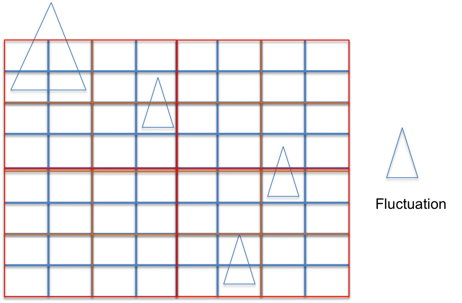
(a) A smooth data field with fluctuations

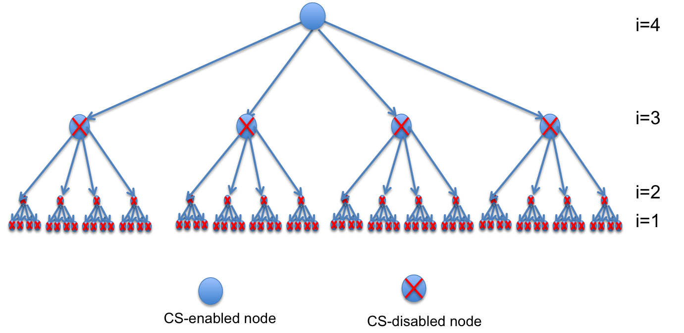
(b) HDACS logical tree

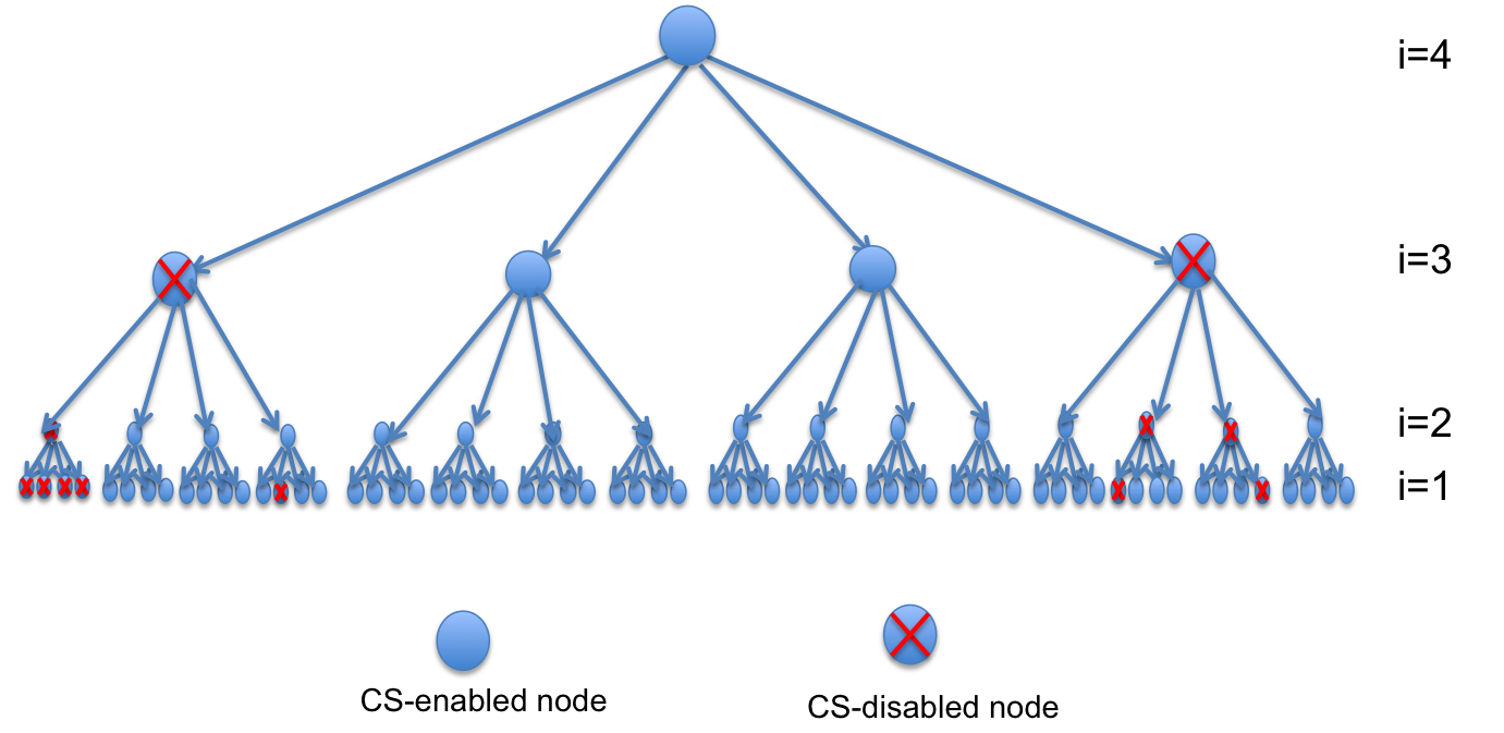
(c) A-HDACS logical tree

Figure 1: An example of a smooth data field with fluctuations and its corresponding logical tree in HDACS and A-HDACS

To better understand this analysis, Fig.1(a) gives a simple example of a smooth data field with a few variations measured by the sensor network in a data aggregation task. Fig.1(b) and Fig.1(c) are its corresponding logical hierarchical trees in HDACS and A-HDACS. The local variations in data field lead to the large value of global sparsity constant $K_{T}$ of the data field, and in HDACS it leads to plenty of nodes to be classified as CS-disabled nodes. However, in the same situation, since in A-HDACS sparsity constants $K_{i}$s are computed based on local variations in each cluster $i$, a large fraction of the CS-disabled nodes in HDACS become CS-enabled nodes in A-HDACS.

V Performance Evaluation

V-A Simulation Settings

We evaluate the performance of the proposed A-HDACS scheme using SIDnet-SWANS [12], a JAVA based sensor network simulation platform. In our experiments we have used multiple network sizes, ranging from 300 to 800 sensor nodes, populated in a fixed field size of $4000*4000m^{2}$ area. The average nodes distribution density varies from $18.75/\text{km}^{2}$ to $50/\text{km}^{2}$. Fig. 2(a) shows a constant data field filled with randomly located Gaussian bumps. It has the maximum height 10 units and decays with 0.01 exponential rate. Fig. 2(b) depicts a smooth data field with a discontinuity along the line $x=y$, where the readings from smooth area are either 10 or 20 plus independent Gaussian noise with zero mean and 0.01 variance.

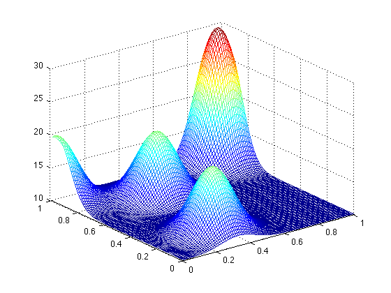
(a) Smooth data field filled with Gaussian bumps

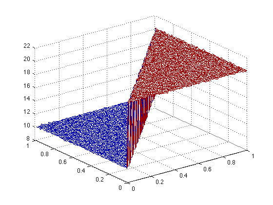
(b) Piecewise data field

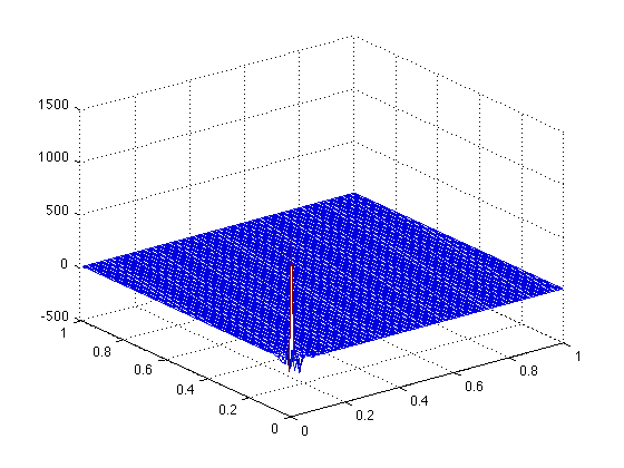
(c) DCT domain of smooth data field filled with Gaussian bumps

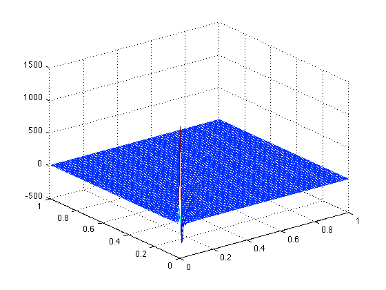
(d) DCT domain of piecewise data field

Figure 2: Data Fields and their corresponding DCT Domain

Besides, Discrete Cosine Transform (DCT) has been used to represent the data field in the transform domain. DCT is a suboptimal transform for sparse signal representation and approaches the ideal optimal transform when the correlation coefficient between adjacent data elements approaches unity [13]. Fig. 2(c) and Fig. 2(d) show the results when data fields are projected into DCT space. As we can see, most signal energy is captured in a very few coefficients, and the magnitudes decay rapidly. Also, note that the DCT signal corresponding to the piecewise data field, shown in Fig. 2(d), has less fluctuations than the signal corresponding to the smooth data field with Gaussian bumps, shown in Fig. 2(c).

V-B The Nodes Distribution

Fig. 3 shows the SIDnet simulation results of A-HDACS and HDACS for two types of data fields with network size 400, where black nodes denote CS-enabled nodes, gray nodes denote that are unable to use CS, and white nodes are the leaf nodes at level one of the aggregation tree. As we can see in Fig3(a), due to the scattered fluctuations present in the data field with Gaussian bumps it is very difficult to obtain sparse signal representation, therefore there are only a few CS-enabled nodes. But still for the clusters in local smooth data areas A-HDACS is able to utilize CS. Fig. 3(b) shows that piecewise data field has a large percent of CS-enabled nodes. CS-disabled nodes are mainly placed around the discontinuity of the line $x=y$. And the clusters away from this line can fully utilize CS. Fig. 3(c) and Fig. 3(d) depict the nodes distribution for both data fields using HDACS. The results are identical: almost no CS can be performed at the lower level except a few nodes at top levels. It demonstrates the significant improvement of CS-enabled nodes in A-HDACS and it is consistent with theoretical analysis in Section IV.

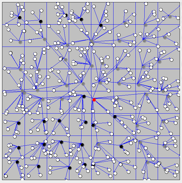
(a) A-HDACS: smooth data field filled with Gaussian bumps

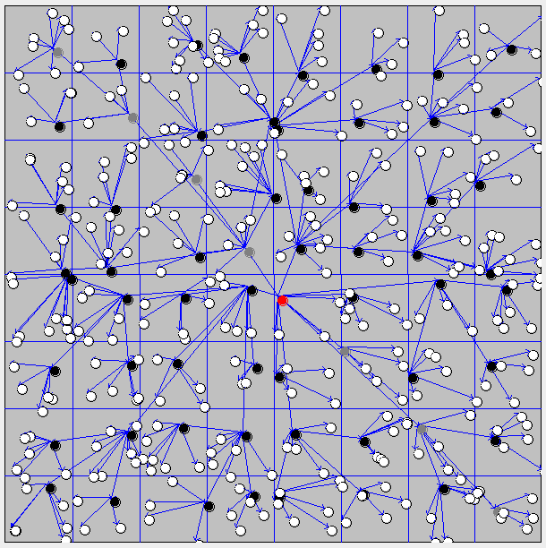
(b) A-HDACS: piecewise data field

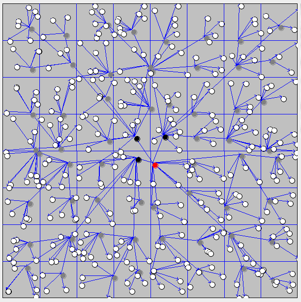
(c) HDACS: smooth data field filled with Gaussian bumps

(d) HDACS: piecewise data field

Figure 3: The SIDnet simulation results of A-HDACS and HDACS with network size 400: black nodes denote CS-enabled nodes, gray nodes denote CS-disabled nodes, white nodes are the leaf nodes on level one, and red node denotes the sink.

V-C Data Recovery Results

Common signals are usually K-compressive – K entries with significant magnitudes and the other entries rapidly decaying to zero. Since K-sparse signal is one requirement of CS, it is necessary to perform signal truncation process. In the simulation, we tested different signal truncation thresholds so as to get as many CS-enabled nodes as possible without compromising too much signal recovery accuracy. Based on the characteristic of DCT signal, truncation threshold is set up as the percentage of the first dominant magnitude.

In the evaluation, Mean Square Error (MSE) of recovered signal in the root node (sink) is defined as the average difference between recovered data and actual reading values for all the sensors. Fig. 4 depicts MSE versus DCT truncation threshold for two types of data field with network size 400. Since small truncation threshold filters out fewer significant entries than larger thresholds, it obtains better MSE. Fig. 4 shows that MSE of the smooth data field with Gaussian bumps is below 0.066 when DCT thresholds are smaller than 0.0225, and it increases dramatically when DCT thresholds are large. In the case of the field with Gaussian bumps, fluctuations in the signal cause increase in the number of DCT coefficients that has significant magnitudes, therefore truncation process is less effective. Relatively, piecewise field has more smooth clustering area with only a few significant entries. Its MSE is under a negligible value when DCT threshold is in the range of $[0.005,0.03]$.

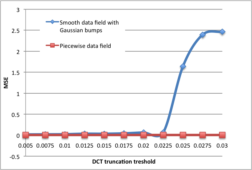
Figure 4: MSE versus DCT truncation threshold with network size 400

In the simulation results presented here onwards, DCT magnitudes bigger than $1\%$ of the first dominant coefficient are preserved. Figs. 5(a) and 5(b) show MSE at each level of the aggregation tree for the two data fields. In both cases, MSE results deteriorate with the increase of levels. This is because the signal truncation errors propagate in the data aggregation hierarchy. In the meanwhile, comparing Fig. 5(a) with Fig. 5(b), overall piecewise data field has smaller errors than the smooth data field with Gaussian bumps. It is due to relatively less fluctuations in the piecewise smooth data field.

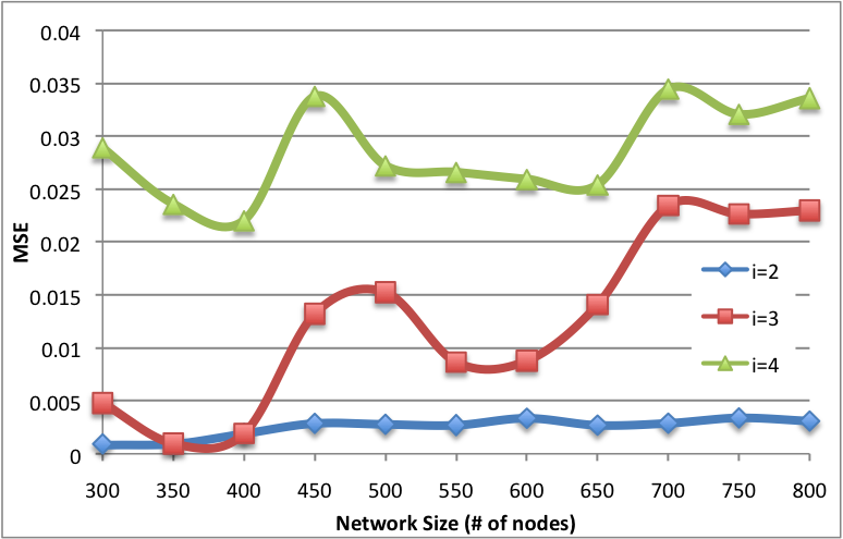
(a) Smooth data field filled with Gaussian bumps

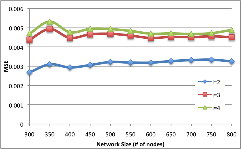
(b) Piecewise data field

Figure 5: Data recovery mean square error (MSE) results at each level

V-D Energy Consumption

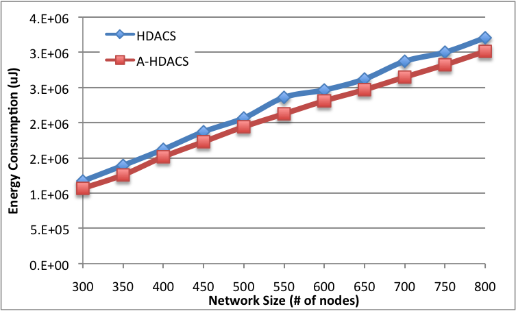
(a) Smooth data field filled with Gaussian bumps

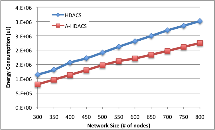
(b) Piecewise data field

Figure 6: Total Transmission Energy Cost versus Different Network Sizes

Since communication operations consumes majority of the battery power, we start counting energy consumption only when data aggregation begins. Fig. 6(a) and Fig. 6(b) show energy consumption versus networks size for two types of data field. A-HDACS consumes only $90.1\%\sim 94.20\%$ energy of HDACS in all the network sizes. Although plenty of fluctuations in the data field affects A-HDACS to apply CS in a certain degree, it still captures the sparsity feature within a few cluster area. But HDACS is insensitive to the local area, when the data field slightly change, it loses its data compression capability. This advantage is obvious, when it comes to the piecewise data field. Fig. 6(b) shows that A-HDACS can save around $23.36\%\sim 30.17\%$ battery power, compared to HDACS. The results demonstrate that significant energy efficiency can be obtained by the proposed technique.

VI Conclusion and Future Work

In this paper, Adaptive Hierarchical Data Aggregation using Compressive Sensing (A-HDACS) has been proposed to perform data aggregation in non-smooth multimodal data fields. Existing CS based data aggregation schemes for WSNs are inefficient for such data fields, in terms of energy consumed and amount of data transmitted. The A-HDACS solution is based on computing sparsity coefficients using signal sparsity of data gathered in local clusters. We analytically prove that A-HDACS enables more clusters to use CS compared to conventional HDACS. The simulation evaluated on SINnet-SWANS also demonstrates the feasibility and robustness of A-HDACS and its significant improvement of energy efficiency as well as accurate data recovery results.

In the future work, more factors will be considered to strength A-HDACS. For example, in our implementations the cluster size is fixed at each level of the hierarchy. It may be possible to further improve communication cost if cluster size itself is also set up depending on the local density of the nodes. Besides, temporal correlations in the data may be exploited to further reduce the amount of data transmitted. Finally, other distributed computing tasks beyond data aggregation, such DFT, DWT, will also be implemented using A-HDACS framework, to take advantage of its power-efficient execution.

References

- [1] R. Rajagopalan and P. K. Varshney, “Data aggregation techniques in sensor networks: A survey,” IEEE Communications Surveys and Tutorials, vol. 8, no. 4, 2006.
- [2] H. Zhang and H. Shen, “Balancing Energy Consumption to Maximize Network Lifetime in Data-Gathering Sensor Networks,” IEEE Transactions on Parallel and Distributed Systems, vol. 20, no. 10, pp. 1526–1539, October 2009.
- [3] H. Jiang, S. Jin, and C. Wang, “Prediction or Not? An Energy-Efficient Framework for Clustering-Based Data Collection in Wireless Sensor Networks,” IEEE Transactions on Parallel and Distributed Systems, vol. 22, no. 6, pp. 1064–1071, June 2011.
- [4] X. Tang and J. Xu, “Optimizing Lifetime for Continuous Data Aggregation With Precision Guarantees in Wireless Sensor Networks,” IEEE Transactions on networking, vol. 16, no. 4, pp. 904–917, August 2008.
- [5] D. L. Donoho, “Compressed Sensing,” IEEE Trans. Inf. Theory, vol. 52, no. 4, 2006.
- [6] R. G. Baraniuk, “Compressive Sensing [lecture notes].” Signal Processing Magazine, IEEE, vol. 24, no. 4, pp. 118–121, 2007.
- [7] [Online]. Available: http://en.wikipedia.org/wiki/Compressed_sensing
- [8] C. Luo, F. Wu, J. Sun, and C. W. Chen, “Compressive Data Gathering for Large-Scale Wireless Sensor Networks.” Beijing, China: MobiCom, September 20-25 2009.
- [9] J. Luo, L. Xiang, and C. Rosenberg, “Does compressed sensing improve the throughput of Wireless Sensor Networks?” no. 1-6. Cape Town, South Africa: In Proceedings of the IEEE International Conference on Communications, May 2010.
- [10] L. Xiang, J. Luo, and A. V. Vasilakos, “Compressed Data Aggregation for Energy Efficient Wireless Sensor Networks,” no. 46. the 8th IEEE SECON, 2011.
- [11] X. Xu, R. Ansari, and A. Khorkhar, “Power-efficient hierarchical Data Aggregation using Compressive Sensing in WSNs.” Budapest, Hungary: IEEE International Conference on Communications (ICC), June 9-13 2013.
- [12] O. C. Ghica. SIDnet-SWANS Manual. [Online]. Available: http://users.eecs.northwestern.edu/~ocg474/SIDnet/SIDnet-SWANS%20manual.pdf
- [13] R. Clarke, “Relation between the karhunen loã¨ve and cosine transforms,” Communications, Radar and Signal Processing, IEE Proceedings F, vol. 128, no. 6, pp. 359 – 360, Nov 1981.