On the Physics of Radio Halos in Galaxy Clusters: Scaling Relations and Luminosity Functions

Abstract

The underlying physics of giant and mini radio halos in galaxy clusters is still an open question. We find that mini halos (such as in Perseus and Ophiuchus) can be explained by radio-emitting electrons that are generated in hadronic cosmic ray (CR) interactions with protons of the intracluster medium. By contrast, the hadronic model either fails to explain the extended emission of giant radio halos (as in Coma at low frequencies) or would require a flat CR profile, which can be realized through outward streaming and diffusion of CRs (in Coma and A2163 at 1.4 GHz). We suggest that a second, leptonic component could be responsible for the missing flux in the outer parts of giant halos within a new hybrid scenario and we describe its possible observational consequences. To study the hadronic emission component of the radio halo population statistically, we use a cosmological mock galaxy cluster catalog built from the MultiDark simulation. Because of the properties of CR streaming and the different scalings of the X-ray luminosity ($L_{\mathrm{X}}$) and the Sunyaev-Zel’dovich flux ($Y$) with gas density, our model can simultaneously reproduce the observed bimodality of radio-loud and radio-quiet clusters at the same $L_{\mathrm{X}}$ as well as the unimodal distribution of radio-halo luminosity versus $Y$; thereby suggesting a physical solution to this apparent contradiction. We predict radio halo emission down to the mass scale of galaxy groups, which highlights the unique prospects for low-frequency radio surveys (such as the LOFAR Tier 1 survey) to increase the number of detected radio halos by at least an order of magnitude.

1 Introduction

The presence of large-scale diffuse radio synchrotron emission in clusters of galaxies proves the existence of relativistic electrons and magnetic fields permeating the intracluster medium (ICM). This diffuse cluster radio emission can be observationally classified into two phenomena: peripheral radio relics, which show irregular morphology and polarized emission and appear to trace merger and accretion shocks, as well as radio halos (see, e.g., Feretti et al., 2012). Radio (mini-)halos (RHs) are characterized by unpolarized radio emission, are centered on clusters and show a regular morphology, resembling the morphology of the thermal X-ray emission. However, the short cooling length of synchrotron-emitting electrons at GHz frequencies ($\lesssim 100$ kpc) challenges theoretical models to explain the large-scale radio emission that extends over several Mpcs and calls for an efficient in-site acceleration process of electrons.

Two principal models have been proposed to explain RHs. In the “hadronic model” the radio emitting electrons are produced in hadronic cosmic ray (CR) proton interactions with protons of the ambient thermal ICM, requiring only a very modest fraction of (at most) a few percent of CR-to-thermal pressure (Dennison, 1980; Vestrand, 1982; Blasi & Colafrancesco, 1999; Dolag & Enßlin, 2000; Miniati et al., 2001b, a; Miniati, 2003; Pfrommer & Enßlin, 2003, 2004b, 2004a; Blasi et al., 2007; Pfrommer et al., 2008; Pfrommer, 2008; Kushnir et al., 2009; Donnert et al., 2010a, b; Keshet & Loeb, 2010; Keshet, 2010; Enßlin et al., 2011). CR protons and heavier nuclei, like electrons, can be accelerated and injected into the ICM by structure formation shocks, active galactic nuclei (AGN) and galactic winds. Due to their higher masses with respect to electrons, CR protons are accelerated more efficiently to relativistic energies and are expected to show a ratio of the spectral energy flux of CR protons to electrons above 1 GeV of about 100, similarly to what is observed in our Galaxy (Schlickeiser, 2002). Additionally, CR protons have a radiative cooling time larger than that of the electrons by the square of the mass ratio and therefore can accumulate in clusters for cosmological times (Völk et al., 1996). In contrast, CR electrons suffer more severe energy losses via synchrotron and inverse Compton emission at particle energies $E\gtrsim 100$ MeV, and Coulomb losses below that energy range.

In the “re-acceleration model”, RHs are thought to be the result of re-acceleration of electrons through interactions with plasma waves during powerful states of ICM turbulence, as a consequence of a cluster merger (Schlickeiser et al., 1987; Giovannini et al., 1993; Gitti et al., 2002; Brunetti et al., 2004; Brunetti & Blasi, 2005; Brunetti & Lazarian, 2007, 2011; Brunetti et al., 2009; Donnert et al., 2013). This, however, requires a sufficiently long-lived CR electron population at energies around 100 MeV which has to be continuously maintained by re-acceleration at a rate faster than the cooling processes. We refer the reader to Enßlin et al. (2011) for a discussion on the strengths and weaknesses of these two models.

RHs can be divided in two classes. Giant radio halos are typically associated with merging clusters and have large extensions, e.g., the Coma RH has an extension of about 2 Mpc. Radio mini-halos are associated with relaxed clusters that harbor a cool core and typically extend over a few hundred kilo-parsecs, e.g., the Perseus radio mini-halo has an extension of about 0.2 Mpc. The observed morphological similarities with the thermal X-ray emission suggests that RHs may be of hadronic origin. In fact, cool-core clusters (CCCs) are characterized by high thermal X-ray emissivities and ICM densities that are more peaked in comparison to non cool-core clusters (NCCCs) that often show signatures of cluster mergers (e.g., Croston et al., 2008). This distinct difference in the ICM density structure of CCCs and NCCCs would be reflected in the morphology of the two observed classes of RHs.

The RH luminosity seems to be correlated to the thermal X-ray luminosity (e.g., Brunetti et al., 2009; Enßlin et al., 2011). However, a large fraction of clusters does not exhibit significant diffuse synchrotron emission at current sensitivity limits. Stacking subsamples of luminous X-ray clusters reveals a signal of extended diffuse radio emission that is below the radio upper limits on individual clusters (Brown et al., 2011) suggesting that at least a subset of apparently “radio-quiet” clusters shows a low-level diffuse emission. Galaxy clusters with the same thermal X-ray luminosity show an apparent bimodality with respect to their radio luminosity. This suggests the existence of a switch-on/switch-off mechanism that is able to change the radio luminosity by more than one order of magnitude. While such a mechanism could be easily realized in the framework of the re-acceleration model (Brunetti et al., 2009), the classical hadronic model predicts the presence of RHs in all clusters. The failure to reproduce the observed cluster radio-to-X-ray bimodality was one of the main criticisms against the hadronic model. Additionally, the classical hadronic model cannot reproduce some spectral features observed in clusters, such as the total spectral (convex) curvature claimed in the Coma RH or the spectral steepening observed at the boundary of some RHs. However, the recent report of spectral flattening with frequency of the RH in A2256 (van Weeren et al., 2012) could easily be accommodated in the hadronic model, which naturally produces such a concave spectrum (Pinzke & Pfrommer, 2010). This raises the interesting question whether such a variability among different sources that are generally classified as “radio halos” signals the presence of richer underlying physics—a question that we will address in this paper.

Enßlin et al. (2011) tried to asses these problems of the classical hadronic model by analyzing CR transport processes within a cluster. While CR advection with turbulently driven flows results in centrally enhanced CR profiles, the propagation in form of CR streaming and diffusion produces a flattening of CR profiles. Hence, different CR transport phenomena may also account for the observed bimodality of the radio luminosity in the hadronic model and may also explain the spectral features observed in some clusters. This has been recently confirmed by Wiener et al. (2013). In particular, by considering turbulent damping, they show that CRs can stream at super-Alfvénic velocities. Note that these phenomena were not considered in earlier analytical works (e.g., Pfrommer & Enßlin, 2004b) as well as in previous hydrodynamic simulations (e.g., Miniati et al., 2001b; Pfrommer et al., 2008; Pinzke & Pfrommer, 2010). A satisfactory theory of CR transport in clusters does not yet exist. However, CR streaming and diffusion may represent an intriguing solution for the issues of the classical hadronic model.

Basu (2012) presented the first scaling relations between RH luminosity and Sunyaev-Zel’dovich (SZ) flux measurements, using the Planck cluster catalogue. While the correlation agrees with previous scaling measurements based on X-ray data, there is no indication for a bimodal cluster population dividing clusters into radio-loud and radio-quiet objects at fixed SZ flux. While the SZ flux correlates tightly with cluster mass, the X-ray luminosity, $L_{\mathrm{X}}$, exhibits a larger scatter. The CCCs predominantly populate the high-$L_{\mathrm{X}}$ tail (at any cluster temperature) and make up approximately half of the radio-quiet objects (Enßlin et al., 2011). This suggests that the switch-on/switch-off mechanism may not operate at fixed $L_{\mathrm{X}}$ but also causes an evolution of that quantity. As the cluster relaxes after a merger, it cools and forms a denser core. Simultaneously, $L_{\mathrm{X}}$ is expected to increase which may simultaneously decrease the radio luminosity owing to the decaying turbulence that is responsible in maintaining the radio emission in either model (that accounts for microscopic CR transport). This has been recently confirmed by Sommer & Basu (2014) and Cassano et al. (2013).

An observational test that is able to disentangle between the hadronic and re-acceleration models is the gamma-ray emission resulting from neutral pion decays, a secondary product of the hadronic CR interaction with protons of the ICM, which is not predicted by the re-acceleration model. Such observational efforts have been undertaken in the last few years (for space-based cluster observations in the GeV-band, see Reimer et al. 2003; Fermi-LAT Collaboration 2010a, b; Han et al. 2012; Fermi-LAT Collaboration 2014; Huber et al. 2013; Prokhorov & Churazov 2014; for ground-based observations in the energy band $\gtrsim 100$ GeV, see Perkins et al. 2006; Perkins 2008; HESS Collaboration 2009b, a; Domainko et al. 2009; Galante et al. 2009; Kiuchi et al. 2009; VERITAS Collaboration 2009; MAGIC Collaboration 2010, 2012; VERITAS Collaboration 2012; HESS Collaboration 2012) without being able to detect cluster gamma-ray emission. Current gamma-ray limits enable us to constrain the average CR-to-thermal pressure to be less than a couple percent, and the maximum CR acceleration efficiency at structure formation shocks to be $<50$ per cent. Alternatively, this may indeed suggest the presence of non-negligible CR transport processes into the outer cluster regions.

An important step towards understanding the generating mechanism of RHs could come from detailed RH population analyses. To date, we know of 53 clusters that harbor RHs (Feretti et al., 2012, for an almost up-to-date list). Only few X-ray flux-limited studies have been conducted that assess the important question of the RH frequency in clusters (Giovannini et al., 1999; Venturi et al., 2008; Kale et al., 2013). Since the number of RHs in such X-ray flux-limited samples is small with typically a few RHs, the conclusions on the underlying physical mechanisms of RHs are not very robust. Fortunately, this is expected to change thanks to the next-generation of low-frequency radio observatories such as the Low Frequency Array (LOFAR). In fact, a deep cluster survey is part of the LOFAR science key projects and expected to provide a large number of radio-emitting galaxy clusters up to redshift $z\approx 1$ (Röttgering et al., 2012). This will hopefully permit to clearly determine the RH phenomenology with respect to cluster properties such as the fractions of radio-loud/quiet, non cool-core/cool-core, and non-merging/merging clusters, and to explore the role of different parameters like the magnetic field, the CR acceleration efficiency, and CR transport properties.

The main scope of this work is to account for CR transport processes in the classical hadronic model and to provide forecasts for future radio surveys. The outline is as follows. In Section 2, we construct a model for the CR proton distribution in clusters that merges results of hydrodynamic cluster simulations and an analytical model for microscopic CR transport processes. In Section 3, we model observed surface brightness profiles of individual RHs within the hadronic scenario and explore the allowable parameter space for CRs and magnetic fields. Motivated by immanent challenges to explain the extent of giant radio halos within the hadronic model, we suggest a new hybrid leptonic/hadronic scenario meant to unify the apparently distinct classes of giant radio halos, mini halos, and steep spectrum radio sources in Section 4. In Section 5, we apply our extended hadronic model to a cosmologically complete mock galaxy cluster catalog built from the MultiDark $N$-body $\Lambda$CDM simulation in Zandanel et al. (2014), hereafter Paper I. We compare the resulting modeled radio-to-X-ray and radio-to-SZ scaling relations to current observations and show how they vary for different choices of our CR and magnetic field parametrizations. In Section 6, we show the radio luminosity functions, compare them to current observational constraints, and provide predictions of the hadronically-generated RHs for the LOFAR cluster survey. Finally, in Section 7, we present our conclusions. In this work, the cluster mass $M_{\Delta}$ and radius $R_{\Delta}$ are defined with respect to a density that is $\Delta=200$ or $500$ times the critical density of the Universe. We adopt density parameters of $\Omega_{\mathrm{m}}=0.27$, $\Omega_{\Lambda}=0.73$ and today’s Hubble constant of $H_{0}=100\,h_{70}$ km s^-1 Mpc^-1 where $h_{70}=0.7$.

2 Cosmic Ray Modeling

We assume a power-law for the spectral distribution of CR protons, $f(R,p)\mathrm{d}p=C(R)p^{-\alpha}\mathrm{d}p$, which is the effective one-dimensional momentum distribution (assuming isotropy in momentum space). The spatial CR distribution $C(R)$ within a galaxy cluster is governed by an interplay of CR advection, streaming, and diffusion. The advection of CRs by turbulent gas motions is dominated by the largest eddy turnover time $\tau_{\mathrm{tu}}\sim L_{\mathrm{tu}}/\upsilon_{\mathrm{tu}}$. Here, $L_{\mathrm{tu}}$ denotes the turbulent injection scale (typically of order the core radius) and $\upsilon_{\mathrm{tu}}$ is the associated turbulent velocity that approaches the sound speed $\upsilon_{\mathrm{s}}$ for transsonic turbulence after a cluster merger and relaxes to small velocities afterwards. As a result of advection into the dense cluster atmosphere, CRs are adiabatically compressed and experience a stratified distribution in the cluster potential. The gradient of the CR number density leads to a net CR streaming motion towards the cluster outskirts. Streaming CRs excite Alfvén waves on which they resonantly scatter (Kulsrud & Pearce, 1969). This isotropizes the CRs’ pitch angles, and thereby reduces the CR bulk speed. Balancing the growth rate of the CR Alfvén wave instability with the wave damping rate due to non-linear Landau damping yields a CR streaming speed of order the Alfvén speed (Felice & Kulsrud, 2001). This increases considerably when balancing it with the turbulent damping rate, which implies an inverse scaling with the CR number density (Wiener et al., 2013). Once CR streaming depletes the CR number density, this causes a run-away process with a rapidly increasing streaming speed that even surpasses the sound speed because the smaller CR number density drives the CR Alfvén wave instability less efficiently. Hence, the crossing time of streaming CRs over $L_{\mathrm{tu}}$ is $\tau_{\mathrm{st}}\sim\chi_{B}\,L_{\mathrm{tu}}/\upsilon_{\mathrm{st}}$ with the streaming velocity given by $\upsilon_{\mathrm{st}}\sim\upsilon_{\mathrm{s}}$ and $\chi_{B}\lesssim 1$ parametrizes the magnetic bending scale. Magnetic bottlenecks for the macroscopic, diffusive CR transport, are critical in lowering the microscopic streaming velocity of CR by some finite factor. Therefore, we can define a turbulent propagation parameter

$$\gamma_{\mathrm{tu}}\equiv\frac{\tau_{\mathrm{st}}}{\tau_{\mathrm{tu}}}=\frac{\chi_{B}\,\upsilon_{\mathrm{tu}}}{\upsilon_{\mathrm{st}}}$$ (1)

that indicates the relative importance of advection versus CR streaming as the dominant CR transport mechanism. After a merger, turbulent advective transport should dominate yielding $\gamma_{\mathrm{tu}}\gg 1$, which results in centrally enhanced CR profiles. In contrast, in a relaxed cluster, CR streaming should be the dominant transport mechanism implying $\gamma_{\mathrm{tu}}\sim 1$ and producing flat CR profiles (for a detailed discussion of these processes, see Enßlin et al., 2011 and Wiener et al., 2013).

We propose here to take the spectral shape of the CR distribution function from cosmological hydrodynamical simulation of clusters (Pinzke & Pfrommer, 2010), which however did not account for CR transport. To include the latter, we adapt the analytical formalism of Enßlin et al. (2011). This results in a model that includes the necessary CR transport physics and is able to predict radio and gamma-ray emission. Note that this approach is not fully self-consistent and points to the necessity of future hydrodynamical simulations to include the effect of CR streaming and diffusion on the CR spectrum.

Figure 1: Left panel. We show our extended model profiles for the normalization of the CR distribution for the NCCC and CCC cases and for different values of $\gamma_{\mathrm{tu}}$. We fix the CR number for the case of $\gamma_{\mathrm{tu}}=100$ using equation (36) of Enßlin et al. (2011), while integrating the cluster volume within $R_{200}$, and require CR number conservation during CR streaming. Right panel. We compare the extended model (adopting $\gamma_{\mathrm{tu}}=100$) with the semi-analytical advection-only case (adopting our GNFW gas profiles and the outer temperature decrease to the simulation-derived model proposed by Pinzke & Pfrommer, 2010) and with the exact analytical solution as in Enßlin et al. (2011), but for our GNFW profiles (adopting $\alpha=2.3$ and $\gamma_{\mathrm{tu}}=100$). Here, the CR profiles are normalized at $C_{0.1}=C(0.1R_{200})$.

To construct such a model, we have to generalize the approach proposed by Enßlin et al. (2011), which uses a $\beta$-profile gas parametrisation, in order to account for different ICM gas profiles, such as our generalized Navarro-Frank-White (GNFW) ICM profiles derived in Paper I from X-ray observations. We also have to include the cluster mass-scaling of the CR normalization obtained from simulations (Pinzke & Pfrommer, 2010). While details are given in Appendix A, we summarize below the main steps. When turbulent advection completely dominates the CR transport, the CR normalization can be written as (Enßlin et al., 2011)

$$C_{\mathrm{adv}}(R)=C_{0}\left(\frac{P_{\mathrm{th}}(R)}{P_{\mathrm{th},0}}\right)^{\frac{\beta_{\mathrm{CR}}}{\gamma}}=C_{0}\eta(R)^{\beta_{\mathrm{CR}}},$$ (2)

where $P_{\mathrm{th}}$ is the thermal pressure, $\beta_{\mathrm{CR}}=(\alpha+2)/3$, $\gamma=5/3$, and we introduced the advective CR profile $\eta(R)=(P_{\mathrm{th}}(R)/P_{\mathrm{th},0})^{1/\gamma}$. Solving the continuity equation for CRs, Enßlin et al. (2011) derive the CR density profile,

$$\rho_{\mathrm{CR}}(R)=\rho_{\mathrm{CR},0}\eta(R)\mathrm{exp}\left(\frac{R}{R_{*}}\right)\,,$$ (3)

where $R_{*}=\gamma_{\mathrm{\mathrm{tu}}}R_{\mathrm{c}}$ and $R_{\mathrm{c}}$ is the characteristic radius, of order the core radius, at which the turbulence is supposed to be injected. Now, we introduce the semi-analytical mass-dependent normalization of the CR profile of Pinzke & Pfrommer (2010) such that

$$\eta(R)=\left(\frac{C_{\mathrm{adv}}(R)}{C_{0}}\right)^{1/\beta_{\mathrm{CR}}}\to\left(\frac{C_{\mathrm{extended}}(R)}{C_{0}}\right)^{1/\beta_{\mathrm{CR}}}\,,$$ (4)

which effectively redefines $C_{\mathrm{adv}}(R)$ by that of our extended model, i.e.,

$$C_{\mathrm{extended}}(R)=\tilde{C}(R)\,\frac{\rho_{\mathrm{gas}}(R)}{m_{\mathrm{p}}}\frac{T(R)}{T_{0}}.$$ (5)

Here, $\rho_{\mathrm{gas}}$ is the ICM gas density and $\tilde{C}(R)$ is the normalization of the CR profile of equation (22) of Pinzke & Pfrommer (2010). We additionally account for the temperature decline toward the cluster periphery, $T(R)$, given by the fit to the universal temperature profile obtained from cosmological hydrodynamical simulations (Pfrommer et al., 2007; Pinzke & Pfrommer, 2010) and deep Chandra X-ray observations (Vikhlinin et al., 2005). Eventually, the CR profile in our extended model is given by

$$C(R)=C_{0}\left(\frac{\rho_{\mathrm{CR}}(R)}{\rho_{\mathrm{CR},0}}\right)^{\beta_{\mathrm{CR}}},$$ (6)

which is valid within $R_{\pm}$ (equation 16), with $\rho_{\mathrm{CR}}$ defined by equation (3) where $C_{\mathrm{extended}}$ enters through our redefinition of $\eta$, and $C(R)=C(R_{\pm})$ for $R>R_{+}$ and $R<R_{-}$, respectively.

The last step is to generalize the case of one CR population with a single spectral index $\alpha$ to include the spectral curvature as suggested by Pinzke & Pfrommer (2010). They model the CR spectrum with three different power-law CR populations with spectral indices of $\alpha_{i}=(2.15,2.3,2.55)$. Our formalism can be easily extended to account for multiple CR populations by extending the terms with a single $\alpha$ to sums over the three spectral indices (Pinzke & Pfrommer, 2010, see Appendix B). However, introducing a sum over $\alpha_{i}$ in equation (2) would make it impossible to solve analytically for $\eta(R)$ in equation (4). For simplicity, we decided to only use $\alpha=2.3$ in this last case. For the highly turbulent cases, i.e., for $\gamma_{\mathrm{tu}}=100$ (1000), we recover the radial shape and normalization of the semi-analytical model of Pinzke & Pfrommer (2010) within 1 per cent (0.1 per cent).

Summarizing, our extended model for the CR distribution function, has the following properties: it accounts for (i) the X-ray-inferred gas profiles and cluster-mass scaling of the gas fraction (see Paper I), in addition to the universal temperature drop in the outskirts of clusters, (ii) a cluster-mass dependent CR normalization and universal CR spectrum as derived from cosmological hydrodynamical simulations, (iii) an effective parametrization of active CR transport processes, including CR streaming and diffusion, which allows us to explore different turbulent states of the clusters in our mock cluster catalog.

In the left two panels of Fig. 1, we show our extended CR normalization for the GNFW gas profile in the NCCC and CCC cases (see Paper I) and for different values of $\gamma_{\mathrm{tu}}$. As expected, when CR streaming is the dominant CR transport mechanism, i.e., for negligible advective turbulent transport or equivalently, $\gamma_{\mathrm{tu}}\sim 1$, the spatial CR profiles are flattened irrespective of the cluster state. While turbulence in NCCCs could be injected by a merging (sub-)cluster, in the case of CCCs, the interaction of the AGN jet or radio lobe with the ambient ICM could be the source of turbulence.

In the right panel of Fig. 1, we compare our extended model profile with the semi-analytical advection-only case (adopting our GNFW gas profiles and the outer temperature decrease to the model proposed by Pinzke & Pfrommer, 2010) and with the exact analytical solution as in Enßlin et al. (2011), but for our GNFW profiles (see Appendix A for details). The profiles are normalized at $0.1R_{200}$. In the case of dominant advective CR transport, our extended model is an excellent match to the semi-analytical model derived from cosmological cluster simulations (Pinzke & Pfrommer, 2010). The main differences between our extended model (and the semi-analytical model) on the one side and the analytical solution on the other side is the inclusion of the simulation-based “reference” profile $\tilde{C}$ for the advection-only case and the universally observed temperature drop towards the outskirts of clusters. Note that the profiles in our extended model are generally more centrally peaked in comparison to the analytical GNFW case, which is due to the enhanced radiative cooling in the Pinzke & Pfrommer (2010) simulations that did not account for AGN feedback. Thanks to the flexible parametrization in our model, this can be easily counteracted by changing $\gamma_{\mathrm{tu}}$ and $\alpha_{\mathrm{B}}$ (representing the magnetic field radial decline, see next section), however, at the expense that these parameters are now degenerate with our assumptions on the CR profile in the advection-dominated regime and other possible effects that we are not considering, such as cluster asphericity.

3 Radio Surface Brightness Modeling

In this section, we apply our model to reproduce the emission characteristics of four well-observed RHs. We provide the synchrotron emissivity $j_{\nu}$, at frequency $\nu$ and per steradian, in Appendix B. The radio surface brightness $S_{\nu}(R_{\perp})$ (in the small-angle approximation) and luminosity $L_{\nu}$, at a given frequency $\nu$, are given by

$$S_{\nu}(R_{\perp}) = 2\int_{R_{\perp}}^{\infty}j_{\nu}(R)\frac{R}{\sqrt{R^{2}-R_{\perp}^{2}}}\mathrm{d}R,$$ (7)

$$L_{\nu} = 4\pi\int\mathrm{d}Vj_{\nu}(R).$$ (8)

The flux is given by $F_{\nu}=L_{\nu}/(4\pi D^{2})$ where $D$ is the luminosity distance to the object. Note that we do not convolve $S_{\nu}$ with the instrumental point spread function unless specified.

For the purpose of this section, we adopt the measured gas and temperature profiles derived from X-ray observations of each cluster. Our extended model includes an overall normalization $g_{\mathrm{CR}}$ of the CR distribution function and the hadronically-induced non-thermal emission (Appendix B). Note that this parameter can be interpreted as a functional that depends on the maximum CR acceleration efficiency, $g(\zeta_{\mathrm{p,max}})$, but only for $\gamma_{\mathrm{tu}}\gtrsim 100$ (Pinzke & Pfrommer, 2010). We will additionally study the CR-to-thermal pressure $X_{\mathrm{CR}}=P_{\mathrm{CR}}/P_{\mathrm{th}}$, where the CR pressure is given by

$$P_{\mathrm{CR}}=\frac{g_{\mathrm{CR}}Cm_{\mathrm{p}}c^{2}}{6}\sum_{i=1}^{3}\Delta_{i}\mathcal{B}_{1/(1+q^{2})}\left(\frac{\alpha_{i}-2}{2},\frac{3-\alpha_{i}}{2}\right).$$ (9)

Here, $c$ is the speed of light, $\mathcal{B}_{x}(a,b)$ denotes the incomplete beta function, $q=0.8$ is the low-momentum cutoff of the CR distribution, and the normalization factors of the individual CR populations are given by $\Delta_{i}=(0.767,0.143,0.0975)$ (Pinzke & Pfrommer, 2010, see also Appendix B).

We assume a scaling of the magnetic field with gas density that is given by

$$B(R)=B_{0}\,\left(\frac{\rho_{\mathrm{gas}}(R)}{\rho_{\mathrm{gas},0}}\right)^{\alpha_{\mathrm{B}}},$$ (10)

where $B_{0}$ is the central magnetic field and $\alpha_{\mathrm{B}}$ describes the declining rate of the magnetic field strength toward the cluster outskirts. Such a parametrization is suggested by cosmological simulations (Dubois & Teyssier, 2008) as well as Faraday rotation measurements (Bonafede et al., 2010; Kuchar & Enßlin, 2011, and references therein).

For our study, we choose the giant radio halos of Coma (Deiss et al., 1997) and Abell 2163 (Feretti et al., 2001; Murgia et al., 2009), both in merging NCCCs, and the radio mini-halos of Perseus (Pedlar et al., 1990) and Ophiuchus (Govoni et al., 2009; Murgia et al., 2009), both in relaxed CCCs. The radio emission of these clusters is representative of a wide class of RHs. Additionally, Perseus, Ophiuchus and Coma are among the most promising clusters for gamma-ray observations (Pinzke & Pfrommer, 2010; Pinzke et al., 2011). We use X-ray-inferred gas densities $\rho_{\mathrm{gas}}$ and temperatures for Coma (Briel et al., 1992), for A2163 and Ophiuchus (Reiprich & Böhringer, 2002), and for Perseus (Churazov et al., 2003). In Table 1, we summarize the main characteristics of these RHs.

To assess the ability of our extended hadronic model to fit the observed surface brightness profiles, we scan our physically motivated parameter space. The free parameters are the magnetic field (parametrized by $B_{0}$ and $\alpha_{\mathrm{B}}$), the turbulent CR propagation parameter ($\gamma_{\mathrm{tu}}$) and the CR acceleration efficiency. Generally, the normalization of the magnetic profile ($B_{0}$) and the CR acceleration efficiency function ($g_{\mathrm{CR}}$) determine the overall normalization of the emission. The radial decline of the magnetic field ($\alpha_{\mathrm{B}}$) and $\gamma_{\mathrm{tu}}$, both determine the shape of the radio profile and, hence, are also degenerate. By scanning the allowed parameter space and asserting Bayesian priors that rely on observational constraints and theoretical considerations about likely parameter combinations for certain classes (mini halos versus giant halos), we will draw conclusions on the applicability of the hadronic model for RHs. In Fig. 2, we show the surface brightness and CR-to-thermal pressure profiles of each cluster together with the allowed $\gamma_{\mathrm{tu}}-\alpha_{B}$ parameter space. All these clusters are modeled at 1.4 GHz and within $R_{200}$, unless differently specified.

Table 1: Radio-halo and mini-halo characteristics.

cluster	$z$	$D$	$L_{1.4~{}\mathrm{GHz}}$	references
Coma	$0.023$	$101$	$0.72$	[1]
A2163	$0.203$	$962$	$15.36$	[2]
Perseus	$0.018$	$78$	$4.40$	[3]
Ophiuchucs	$0.028$	$121$	$0.19$	[2]

Note. Top two rows correspond to giant radio halos, while the bottom two rows are radio mini-halos. $D$ is the luminosity distance in units of $h_{70}^{-1}$ Mpc and $L_{1.4~{}\mathrm{GHz}}$ is the observed radio luminosity at 1.4 GHz in units of $10^{31}$ $h_{70}^{-2}$ erg s^-1 Hz^-1. References: [1] Deiss et al. (1997) [2] Murgia et al. (2009) [3] Pedlar et al. (1990).

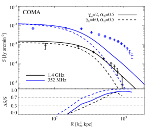
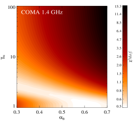
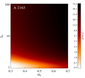
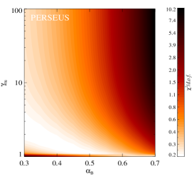
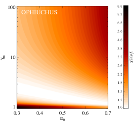
Figure 2: Surface brightness modeling of the RHs in Coma, Abell 2163, Perseus and Ophiuchus. The left and middle panels show the RHs’ azimuthally averaged surface brightness profiles and the corresponding CR-to-thermal pressure profiles $X_{\mathrm{CR}}(r)$, respectively. Representative hadronic model parameters that fit the data well (solid) are compared to parameter choices that will be used in the second part of the paper (dashed, Sects. 5 and 6), which addresses RH statistics. While radio mini-halos can be fit by either set of parameters, for the latter choice of parameters, the hadronic model is not able to explain the emission in the outer parts of giant radio halos and would need a secondary, leptonic component (see text for details). This is exemplified in the lower left panels for Coma and Abell 2163 that show the fraction of missing surface brightness for these parameter choices. In the middle panels, we additionally mark the RHs’ radial extension by a vertical line. The panels on the right show the reduced-$\chi^{2}$ values of our model fits to the data in the $\gamma_{\mathrm{tu}}-\alpha_{B}$ parameter space. Regions of parameter space with reduced-$\chi^{2}$ values substantially larger than unity are excluded by the data while values much smaller than unity may point to an overestimate of the uncertainty intervals. Note that different parameter values that yield almost the same surface brightness profiles may result in very different $X_{\mathrm{CR}}$ profiles. In the case of Abell 2163 and Ophiuchus, we adopt a 10 per cent uncertainty range instead of the errors reported by Murgia et al. (2009) to account for additional systematic uncertainties, e.g., residual point source contamination. For Perseus, we show the mini-halo data only for the range that is unaffected by residual point sources (Pedlar et al., 1990) and adopt a 10 per cent uncertainty budget.

3.1 The Coma radio halo

The giant radio halo in Coma has a morphology remarkably similar to the extended X-ray thermal bremsstrahlung emission, although the radio emission declines more slowly towards the cluster outskirts (Briel et al., 1992; Deiss et al., 1997). The morphology is non-spherical, showing an elongation in the East-West direction. The full-width half maximum (FWHM) of the radio beam is $0.156$ deg (Deiss et al., 1997), almost two orders of magnitude larger than the angular resolution of the X-ray observation of Briel et al. (1992). Thus, we apply a Gaussian smoothing to our theoretical surface brightness of equation (7) with $\sigma_{\mathrm{smoothing}}=FWHM_{\mathrm{radio}}/2.355$.

We investigate different values for $\alpha_{\mathrm{B}}\in[0.3,0.7]$ and $\gamma_{\mathrm{tu}}\in[1,100]$. First, we determine the CR number for $\gamma_{\mathrm{tu}}=100$ using equation (36) of Enßlin et al. (2011) while integrating the cluster volume within $R_{200}$. Then, we require CR number conservation during CR streaming (for CR energies $E>$ GeV where Coulomb cooling is negligible for CR protons), which is realized in our model by lowering the values of $\gamma_{\mathrm{tu}}$. Fixing the central magnetic field $B_{0}=5$ $\mu$G (Bonafede et al., 2010), we use $g_{\mathrm{CR}}$ as normalization factor to match the radio observations. The study of the $\gamma_{\mathrm{tu}}-\alpha_{B}$ parameter space shown in Fig. 2 (top right panel) demonstrates the necessity of low values of $\gamma_{\mathrm{tu}}$ to match the data, i.e., very flat CR profiles. An example of such a good match to the data is obtained for $\gamma_{\mathrm{tu}}=2$ and $\alpha_{\mathrm{B}}=0.5$ (top left panel). Values as high as $\gamma_{\mathrm{tu}}\approx 4$ still provide an acceptable fit, however, at the expense of a shallower decline of the magnetic field profile (smaller $\alpha_{\mathrm{B}}$) as a function of cluster-centric radius. With such values, we can recover the shape of the radio surface brightness as well as the total radio luminosity with a maximal relative deviation of about 25 per cent.

The gamma-ray flux (Appendix C) within $R_{200}$ for the parameter combination $\gamma_{\mathrm{tu}}=2$ and $\alpha_{\mathrm{B}}=0.5$ and for energies above 100 MeV (100 GeV) is $F_{\gamma}=2.4\times 10^{-9}$ ($8.7\times 10^{-13}$) cm^-2 s^-1. We note that our modeled gamma-ray flux $F_{\gamma}(>500~{}\mathrm{MeV})=6.9\times 10^{-10}$ cm^-2 s^-1 formally violates the upper limit recently set with the Fermi-LAT data of $F_{\gamma,UL}(>500~{}\mathrm{MeV})=4\times 10^{-10}$ cm^-2 s^-1 (Fermi-LAT Collaboration, 2014). However, this upper limit has been obtained for the advection-only case (Pinzke & Pfrommer, 2010), which is significantly more peaked than the streaming-dominated $\gamma_{\mathrm{tu}}=2$ case considered here and , thus, it is not directly applicable. Note also that for slightly higher values of $\gamma_{\mathrm{tu}}$, i.e., a more centrally concentrated CR distribution, the radio and gamma-ray yield would be increased (assuming CR number conservation). However, in order to match the observed radio synchrotron profiles, we have to decrease the CR normalization (parametrized by $g_{\mathrm{CR}}$). This causes the associated gamma-ray flux also to be reduced to a level that is low enough to easily circumvent the gamma-ray constraints. E.g., for the parameter combination $\gamma_{\mathrm{tu}}=3$ and $\alpha_{\mathrm{B}}=0.4$, we obtain $F_{\gamma}=1.3\times 10^{-9},3.9\times 10^{-10}$, and $4.9\times 10^{-13}$ cm^-2 s^-1 for energies above 100 MeV, 500 MeV, and 100 GeV, respectively. In principle, CR streaming should cause the CR spectrum to steepen (Wiener et al., 2013). This may then considerably weaken these constraints as a result of the convex spectral curvature since the gamma-ray emission probes the high-energy tail of the CR distribution that is suppressed in this picture in comparison to the lower-energy protons that the radio emission is sensitive to (see MAGIC Collaboration, 2012, for an extended discussion of this point).

However, such low values of $\gamma_{\mathrm{tu}}$ challenge the picture that only clusters that are characterized by a highly turbulent state can host giant radio halos. For illustration, in Fig. 2, we additionally show the radio surface brightness for $\gamma_{\mathrm{tu}}=60$ and $\alpha_{\mathrm{B}}=0.5$; the corresponding gamma-ray flux above 100 MeV (100 GeV) is $F_{\gamma}=5.4\times 10^{-10}$ ($1.9\times 10^{-13}$) cm^-2 s^-1. Clearly, the hadronic model is not able to explain the emission in the outer halo parts and would need a secondary component to fill in the “missing” hadronic radio emission. This is exemplified in the lower plot of the top left panel of Fig. 2, which shows the fraction of missing surface brightness as a function of radius and accumulates to a total missing power of about 35 per cent.

The much more extended RH profile at 352 MHz represents a serious challenge for our extended hadronic model (Brunetti et al., 2012). We complement our RH modeling at high frequencies (1.4 GHz) with modeling of the new data at 352 MHz (Brown & Rudnick, 2011). To this end, we use a novel $352$ MHz surface brightness profile that was corrected for residual point-source contamination by applying the multi-resolution filtering technique described in Rudnick (2002) as well as adopting the X-ray center for the RH profile (Rudnick, priv. comm.). The resulting profile (shown in blue in Fig. 2) declines at a slightly faster rate towards the outskirts than the profile used by Brunetti et al. (2012). More importantly, there is considerable azimuthal variation in the halo profile (see Fig. 4 of Brown & Rudnick, 2011 and also our discussion about RH asphericity in the next section), which would eventually have to be modeled through hydrodynamical cluster simulations but which is beyond the scope of this work.

As shown by the two model realizations in Fig. 2, the (extended) hadronic model cannot account for the total emission at $352$ MHz for any value in the ($\gamma_{\mathrm{tu}}$, $\alpha_{\mathrm{B}}$) parameter space; in agreement with the findings of Brunetti et al. (2012). At the same time, our analysis at 1.4 GHz confirms the result by the VERITAS Collaboration (2012) who also conclude that the hadronic model for the Coma RH is a viable explanation for magnetic field estimates inferred by Faraday rotation measure studies (Bonafede et al., 2010) and is not challenged by Fermi upper limits on the gamma-ray emission. However, this model agreement is bought at the expense of flat CR profiles (i.e., low $\gamma_{\mathrm{tu}}$ values) that are contrary to the expectation of turbulent clusters to host giant radio halos (i.e., high $\gamma_{\mathrm{tu}}$ values) as proposed by Enßlin et al. (2011). Note that Wiener et al. (2013) arrive at a different conclusion and find that the increase of turbulence promotes outward streaming more than inward advection, thus enabling flat CR distributions in turbulent clusters. However, this does not help in the case of the 352 MHz data, where, as discussed above, not even a flat CR profile would suffice to explain the observed emission within the hadronic scenario. These finding hint at the necessity of a second, leptonic component (within the general framework of the hadronic model) that fills in the patchier emission in the peripheral, low-surface brightness regions of the halo (Pfrommer et al., 2008), in particular at low frequencies (see Fig. 3 of Brown & Rudnick, 2011). We will return to this point in Section 4.

3.2 The radio halo in Abell 2163

The morphology of the giant radio halo in Abell 2163 is also closely correlated to the cluster’s thermal X-ray structure. As in Coma, the radio emission declines towards the cluster outskirts at a slower rate in comparison to the thermal X-ray emission (Feretti et al., 2001). The morphological appearance is non-spherical, with an elongation in the East-West direction. We use the surface brightness map provided by Murgia et al. (2009) for which the synthesized radio beam can be approximated by a circular Gaussian with $FWHM_{\mathrm{radio}}=62\arcsec$. Again, $FWHM_{\mathrm{radio}}$ is larger than the angular resolution of the ROSAT observation and the corresponding gas density profile. Converted to physical scale, $\sigma_{\mathrm{smoothing}}$ is of the order of that of Coma because of the larger distance of Abell 2163. Hence, we also apply Gaussian smoothing.

We follow the same procedure as in Coma, and adopt a central magnetic field strength of $B_{0}=5~{}\mu$G. Similar to the case of Coma (in fact even more extremely) only very low values of $\gamma_{\mathrm{tu}}$ provide a good match to the data. In Fig. 2, we show the case of $\gamma_{\mathrm{tu}}=1$ and $\alpha_{\mathrm{B}}=0.3$, i.e., the flattest possible surface brightness. With this choice of parameters, we recover the emission shape and the total luminosity within about 15 per cent. The corresponding gamma-ray flux within $R_{200}$ is $F_{\gamma}(>100~{}\mathrm{MeV})=4.2\times 10^{-10}$ cm^-2 s^-1, about two orders of magnitude lower than the upper limit obtained by Fermi-LAT (Fermi-LAT Collaboration, 2010b), and $F_{\gamma}(>100~{}\mathrm{GeV})=1.5\times 10^{-13}$ cm^-2 s^-1.

As for Coma, in Fig. 2, we show the model surface brightness for the parameter combination $\gamma_{\mathrm{tu}}=60$ and $\alpha_{\mathrm{B}}=0.5$. The corresponding gamma-ray flux above 100 MeV (100 GeV) is $F_{\gamma}=5.9\times 10^{-11}$ ($2.2\times 10^{-14}$) cm^-2 s^-1. The lower panel shows the fraction of missing surface brightness of our model to explain the data as a function of radius. That fraction accumulates to a total missing power of about 80 per cent for the giant radio halo.

3.3 The Perseus radio mini-halo

The diffuse radio emission in Perseus is the best known example of a radio mini-halo (Pedlar et al., 1990) and Perseus itself is among the best studied clusters in X-rays (e.g., Churazov et al., 2003; Fabian et al., 2006, 2011). As for the two radio halos, the Perseus radio morphology resembles that in the X-rays. We proceed as before, but now adopt a higher central magnetic field strength of $B_{0}=10$ $\mu$G. Such a larger $B_{0}$ is expected in a CCC with its higher central gas density, implying a larger adiabatic compression factor of the magnetic field during the condensation of the cool core (see the MAGIC Collaboration, 2010, 2012, for a discussion on the Perseus magnetic field).

Our parameter space study of $\gamma_{\mathrm{tu}}$ and $\alpha_{\mathrm{B}}$ favors low $\gamma_{\mathrm{tu}}$ values—in accordance with our expectation for mini-halos. However, a large region of that parameter space, up to $\gamma_{\mathrm{tu}}=100$, can equally well fit the data. The coloring of the goodness of fit (reduced $\chi^{2}$) in the $\gamma_{\mathrm{tu}}-\alpha_{\mathrm{B}}$ plane shows the anti-correlation of $\gamma_{\mathrm{tu}}$ and $\alpha_{\mathrm{B}}$: large $\gamma_{\mathrm{tu}}$ values (peaked CR profiles) and low $\alpha_{\mathrm{B}}$ values (flat magnetic profiles) combine to match the observed surface brightness profile and vice versa.

In Fig. 2, we show the two parameter combinations ($\gamma_{\mathrm{tu}}=3$, $\alpha_{\mathrm{B}}=0.4$) and ($\gamma_{\mathrm{tu}}=100$, $\alpha_{\mathrm{B}}=0.3$). Both model realizations nicely recover the surface brightness profile and the total luminosity within 10 per cent. The gamma-ray flux within $R_{200}$ for the $\gamma_{\mathrm{tu}}=3$ case and for energies above 100 MeV (100 GeV) is $F_{\gamma}=1.4\times 10^{-8}$ ($5.1\times 10^{-12}$) cm^-2 s^-1. Adopting $\gamma_{\mathrm{tu}}=100$ and $\alpha_{\mathrm{B}}=0.3$, the corresponding gamma-ray flux above 100 MeV (100 GeV) is $F_{\gamma}=4.9\times 10^{-9}$ ($1.8\times 10^{-12}$) cm^-2 s^-1. Note that Fermi-LAT measured the gamma-ray flux above 100 MeV of the central galaxy NGC 1275 to $2\times 10^{-7}$ cm^-2 s^-1 (Fermi-LAT Collaboration, 2009), well above our model predictions due to hadronically produced diffuse gamma-ray emission that is expected to mostly glow from the core region of the cluster.

We can compare these predictions with the upper limit above 1 TeV, and for a region within $0.15$ deg around the cluster center, recently obtained by the MAGIC Collaboration (2012). For $\gamma_{\mathrm{tu}}=3$ ($\gamma_{\mathrm{tu}}=100$), we obtain a flux of $F_{\gamma}(>1~{}\mathrm{TeV},<0.15~{}\mathrm{deg})=7.3\times 10^{-14}$ ($5.5\times 10^{-14}$) cm^-2 s^-1, which is well below the upper limit of the MAGIC collaboration, $F_{\gamma,\mathrm{UL}}(>1~{}\mathrm{TeV},<0.15~{}\mathrm{deg})\approx 1.4\times 10^{-13}$ cm^-2 s^-1. Note also that, in the case of $\gamma_{\mathrm{tu}}=100$, we obtain a maximum CR acceleration efficiency multiplier of $g(\zeta_{\mathrm{p,max}})=0.52$, about half of the value adopted by Pinzke & Pfrommer (2010). Note that adopting $g(\zeta_{\mathrm{p,max}})=1$ results in slightly smaller gamma-ray luminosities in comparison to those predicted by Pinzke & Pfrommer (2010) and Pinzke et al. (2011) because we additionally account for the central temperature dip and as well as the decrease towards larger radii.

3.4 The Ophiuchus radio mini-halo

The Ophiuchus cluster has been widely studied both in radio and X-rays in the last few years because of the claimed presence of a non-thermal hard X-ray tail (Eckert et al., 2008; Fujita et al., 2008; Govoni et al., 2009; Murgia et al., 2009; Pérez-Torres et al., 2009; Nevalainen et al., 2009; Murgia et al., 2010; Million et al., 2010). It was classified as a merging cluster by Watanabe et al. (2001), but more recently Fujita et al. (2008) did not find any evidence of merging and, on the contrary, classified it as one of the hottest clusters with a cool-core (see also Million et al., 2010). To simplify modeling, we neglect the small central temperature dip for radii $r<30\,h_{70}^{-1}$ kpc and adopt a constant central temperature. (Owing to its small size, the cool core region has no influence on the resulting radio surface brightness.) Again, the radio mini-halo morphology displays similarities with the thermal X-ray emission. For our modeling, we use the surface brightness profile provided by Murgia et al. (2009).

We proceed as before, adopting a central magnetic field value of $B_{0}=10$ $\mu$G. Similarly to Perseus, low $\gamma_{\mathrm{tu}}$ values are favored, as expected for mini-halos. However, large regions of the parameter space provide excellent fits to the data. In Fig. 2, we show the two parameter combinations ($\gamma_{\mathrm{tu}}=3$, $\alpha_{\mathrm{B}}=0.4$) and ($\gamma_{\mathrm{tu}}=100$, $\alpha_{\mathrm{B}}=0.3$). For those, we recover the surface brightness profile and the total luminosity within 20 per cent. The gamma-ray flux within $R_{200}$ for the $\gamma_{\mathrm{tu}}=3$ case and for energies above 100 MeV (100 GeV) is $F_{\gamma}=1.3\times 10^{-10}$ ($4.9\times 10^{-14}$) cm^-2 s^-1. Adopting $\gamma_{\mathrm{tu}}=100$ and $\alpha_{\mathrm{B}}=0.3$, the corresponding gamma-ray flux above 100 MeV (100 GeV) is $F_{\gamma}=8.3\times 10^{-11}$ ($3.1\times 10^{-14}$) cm^-2 s^-1. The gamma-ray flux is, in both cases, about two orders of magnitude lower than the upper limit obtained by Fermi-LAT (Fermi-LAT Collaboration, 2010b). Note also that in the case of $\gamma_{\mathrm{tu}}=100$ we obtain a maximum CR acceleration efficiency multiplier of $g(\zeta_{\mathrm{p,max}})=0.014$.

4 Discussion: a hybrid scenario for Giant and Mini Radio Halos?

In order to cleanly assess the possibility of the hadronic model to alone explain the RH data, we only considered the hadronically-induced radio emission component in the preceding section. Hence, by construction, we neglected other (leptonic) emission components, such as reaccelerated electrons. We now address possible biases that may have affected our previous conclusions.

4.1 Biases of the hadronic model of radio halos

(i) Merging clusters are not spherically symmetric as can be seen in Coma and Abell 2163, requiring inherently non-spherical modeling. In order to reproduce the more extended radio emission relative to the thermal X-ray emission, the non-thermal clumping factor, $C_{\mathrm{non-th}}$, needs to be larger than its thermal analogue, $C_{\mathrm{th}}$, in concentric spherical shells, where we defined those statistics by

$$C_{\mathrm{non-th}} = \left\langle\rho_{\mathrm{gas}}C\right\rangle/\left\langle\sqrt{\rho_{\mathrm{gas}}C}\right\rangle^{2},$$ (11)

$$C_{\mathrm{th}} = \left\langle\rho_{\mathrm{gas}}^{2}\right\rangle/\left\langle\rho_{\mathrm{gas}}\right\rangle^{2}.$$ (12)

This manifests itself, e.g., in the large-scale morphology of the radio surface brightness emission, which is more elongated than its counterpart in thermal X-rays, but also on scales smaller than the radio beam. In our phenomenological modeling, we allow for those deviations by means of the parameters $\gamma_{\mathrm{tu}}$ and $\alpha_{\mathrm{B}}$ for the CRs and magnetic fields, respectively. While this approach is well suited to describe large-scale anisotropies, it may be inadequate to model small-scale inhomogeneities such as CR trapping in magnetic mirrors through the second adiabatic invariant and needs to be carefully quantified in future work.

(ii) Adopting the simulation-derived $\tilde{C}$ profile (Pinzke & Pfrommer, 2010) for our extended model may have biased the inner slope of the CR density profile to become too steep due to the overcooling problem of purely radiative simulations. This produces cluster cores that are too dense (in comparison to observations), which also should overestimate the rate of adiabatic compression that is experienced by the CR population during the formation of the cooling core. Hence, the resulting values of $\gamma_{\mathrm{tu}}$ are then biased low in comparison to a potentially shallower slope of the inner CR profile. To quantify the last point, we try to reproduce the Coma surface brightness at 1.4 GHz using a model without $\tilde{C}$. We find that values as high as $\gamma_{\mathrm{tu}}\approx 8$ can be accommodated. However, $\gamma_{\mathrm{tu}}=1$ still represents the best match to the data, demonstrating that the problem can be weakened but not circumvented even in this case of a cored CR profile.

(iii) Considering the case of advection-dominated CR transport ($\gamma_{\mathrm{tu}}\gtrsim 100$), which only allows for a good match to the mini-halo data of Perseus and Ophiuchus, the $g_{\mathrm{CR}}$ parameter can be interpreted as the maximum CR acceleration efficiency used in Pinzke & Pfrommer (2010). If the cluster CR population is mainly accelerated in cosmological structure formation shocks, then this value should depend on the mass accretion history and should be approximately universal, i.e., similar for all clusters. We find $g_{\mathrm{CR,Perseus}}=0.52$ and $g_{\mathrm{CR,Ophiuchus}}=0.014$, because we fixed $B_{0}=10$ $\mu$G in both cases and used $g_{\mathrm{CR}}$ as normalization. This discrepancy can be resolved by increasing/lowering the central magnetic field in Perseus/Ophiuchus to $B_{0,\mathrm{Perseus}}\approx 20$ $\mu$G and $B_{0,\mathrm{Ophiuchus}}\approx 1$ $\mu$G. We note, however, that without the guidance of cosmological cluster simulations that include CR transport, the data does not yet constrain $\gamma_{\mathrm{tu}}$.

The small cluster sample analyzed here is only meant to serve as a proof of concept and to show the viability of matching observed representative RH data with our extended hadronic model. However, it seems unlikely that the biases discussed above severely affect our findings that the extended hadronic model successfully reproduces the main morphological characteristics of radio mini-halos with a wide range of possible values for $\gamma_{\mathrm{tu}}$ and without violating gamma-ray constraints. In contrast, the hadronic model appears to fail in explaining the radio emission in the outskirts of the Coma RH at low frequencies and requires a flat CR distribution both in Coma and in A2163 at 1.4 GHz. This motivates us to consider a modification of this purely hadronic model in explaining RHs.

4.2 Hybrid hadronic-leptonic model

Within the hadronic scenario, there emerges a plausible physical solution to this observational challenge. We suggest that the rich phenomenology of RHs may be a consequence of two different radio emission components—one of which is induced by hadronic interactions and the other is of leptonic origin (Pfrommer et al., 2008). There are a number of plausible processes for the latter. These includes turbulent re-acceleration of primary or secondary (hadronically produced) electrons (Brunetti & Lazarian, 2011) or re-acceleration of fossil electrons by means of diffusive shock acceleration (Kang & Ryu, 2011; Kang et al., 2012; Pinzke et al., 2013). The fossil electron population may originate from the time-integrated and successively cooled population of directly injected electrons at strong structure formation shocks that the gas experienced trough it cosmic accretion history. Alternatively, a seed population of relativistic electrons could be provided by the time-integrated action of AGN feedback or by supernova-driven galactic winds. Depending on relative strength of the different components, this scenario would imply various halo phenomena:

1. A dominating hadronic component manifests in form of radio mini-halos in CCCs (Pfrommer & Enßlin, 2004b).

2. When the leptonic component dominates, we should have steep spectrum halo sources (such as A520, Brunetti et al., 2008), some of which could be produced by giant radio relic sources projected onto the main cluster (Skillman et al., 2013).

3. The case of both components significantly contributing to the diffuse radio emission results in giant radio halos, with the hadronic component dominating in the center and the leptonic emission taking over in the outer parts. The peripheral regions of merging clusters experience an especially high level of kinetic pressure contribution (Lau et al., 2009; Battaglia et al., 2012) that manifests in form of subsonic turbulence (as suggested observationally by Schuecker et al., 2004 or theoretically by Subramanian et al., 2006; Dolag et al., 2005; Ryu et al., 2008) and a complex network of shocks (Ryu et al., 2003; Pfrommer et al., 2006, 2008; Skillman et al., 2008; Vazza et al., 2009). Depending on the merger geometry and dynamical stage, as well as on the electron acceleration efficiencies of these non-equilibrium processes and the CR streaming speeds, we would expect the development of a (fuzzy) transition region between hadronic and leptonic component. This generalizes the simulation-inspired model by Pfrommer et al. (2008) who propose that primary electron substantially contribute to the peripheral RH emission.

A detailed implementation of this hybrid scenario would depend very much on the precise characterization of a given cluster. This goes beyond the scope of the present work, which mainly explores the possible observational consequences of the hadronic component for future radio surveys that are implied by our extended model. Nevertheless, we sketch possible observational implications of a hybrid hadronic-leptonic scenario in the following subsection.

4.3 Observational implications

4.3.1 Spectral and morphological variability

In mini-halos and in the centers of giant halos, where the hadronic component dominates in our picture, we would naively expect at most modest spectral variations. This is because these regions average over sufficiently many fluid elements, each of which experienced its characteristic shock history during the cluster assembly. However, when averaged over the ensemble, this produces a CR population that has a nearly universal spectrum (Pinzke & Pfrommer, 2010). However, CR streaming and diffusive transport may cause a possible spectral steepening in the cluster core region because more energetic CRs diffuse/stream faster. This would then imply spatial variations of the CR spectral index and, hence, spatially varying radio emission throughout the cluster (core region) when taking the CR advection effects into account, which would mix regions of different CR spectral properties. In regions where the leptonic component dominates (such as the outer regions of giant halos or steep spectrum halo sources), we expect substantial spectral and morphological variations in the radio maps. This is because of the intermittency of the acceleration process (acceleration at discrete weak shocks or turbulent acceleration), the expected distribution of Mach numbers or CR momentum diffusion coefficient, respectively, and the comparably short electron cooling time ($\sim 100$ Myr). Interestingly, this compares well with the large azimuthal scatter of different sector profiles of the Coma halo, Fig. 4 of Brown & Rudnick (2011), and fronts (primarily towards the West) in their high-resolution surface brightness map, which may indicate the transition from the hadronic to the leptonic emission component. In particular, the relative inefficiency of shock acceleration at weak shocks or turbulent acceleration generates steeper radio spectra in the leptonically dominated regions. Hence, this would naturally imply a radial spectral steepening and cause substantial morphological and spectral variation in the outer regions of giant halos. The increasing fraction of the leptonic component towards lower frequencies may then imply a larger halo size with decreasing observational frequency.

4.3.2 Halo switch-on/-off mechanism and the radio-X-ray bimodality

Clearly, a cluster merger injects turbulence and shocks that could both accelerate fossil electrons and switch the leptonic component on. On the other hand, CR advection produces centrally enhanced CR profiles because of adiabatic compression of CRs for radial eddies. The energetization and transport of CRs to the central halo regions implies a lightening up of the hadronic emission component. For the leptonic component, the halo switch off is faster or comparable to the dynamical time scale, $t_{\rm dyn}\sim t_{\rm H}/\sqrt{\Delta}\sim 1\,\mathrm{Gyr}\Delta_{100}^{-1/2}$, where $t_{\rm H}=10$ Gyr, $\Delta_{100}=\rho/(100\bar{\rho})$. In the case of diffusive shock acceleration of fossil electrons, the radio emission will be shut off within a CR electron cooling time ($t_{\mathrm{cool}}\sim 100$ Myr) if the acceleration source ceases, i.e., when shocks have dissipated all the energy. In the case of the turbulent re-acceleration model, the turbulence decays on a few eddy turnover time scales on the injection scale which should take somewhat longer. The hadronic emission component is also expected to decrease substantially once turbulent pumping of CRs ceases and CRs are set free to stream, which results in a net CR flux towards the external cluster regions. The accompanying flattening of the CR profile implies a lowering of the hadronic radio emission because the CRs see a smaller target density in the outer parts. This should lead naturally to a bimodality of radio synchrotron emissivities due to hadronic and leptonic halo components.

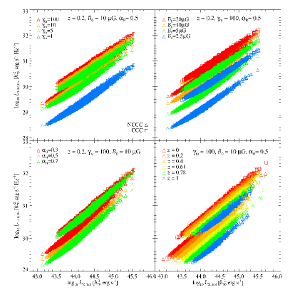
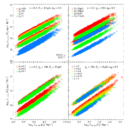
Figure 3: Radio-to-X-ray and radio-to-SZ scaling relations as predicted by our extended CR model. In the left panel, we show how the $L_{1.4~{}\mathrm{GHz}}-L_{\mathrm{X,bol}}$ relation varies upon changing different parameters. In the right panel, we show the same, but for the $L_{1.4~{}\mathrm{GHz}}-Y_{\mathrm{SZ},500}$ relation. Note that in each plot there are two separated populations for each model realization, shown with the same color but different symbols. The upper sets of points (squares) correspond to the CCC population while the lower sets (triangles) correspond to NCCCs. The plot labels indicate those parameters which are kept fixed. We also fix the $g_{\mathrm{CR}}$-normalization parameter to 0.5 for all cases. See main text for further details.

5 Scaling Relations

As introduced in Section 1, there exist an apparent bimodality between the radio and X-ray cluster emission. Clusters with a given X-ray luminosity can either host RHs or show an absence of diffuse radio emission (e.g., Brunetti et al., 2009; Enßlin et al., 2011). More recently, a study of the radio-to-SZ scaling relation revealed the absence of a strong bimodality dividing the cluster population into radio-loud and radio-quiet clusters (Basu, 2012; Cassano et al., 2013; Sommer & Basu, 2014). Since $Y_{\mathrm{SZ}}$ correlates more tightly with cluster mass than $L_{\mathrm{X}}$, this may indicate that the larger scatter of $L_{\mathrm{X}}$ correlates with the scatter of the radio luminosity in such a way that it produces a bimodality; but as a result of a second (hidden parameter) rather than the cluster mass. In this section, we investigate these two scaling relations in the framework of our extended hadronic scenario.

In the following, we apply our model to the complete cosmological mock cluster catalog build from the MultiDark $N$-body simulation in our Paper I. For each object in the sample, we use the cluster mass, a dynamical disturbance parameter (the normalized distance of the halo center and the center of mass) for sorting the cluster into the CCC/NCCC populations, and a phenomenologically assigned ICM density to calculate the radio (and gamma-ray) emission.

5.1 Exploring the parameter space of scaling relations

In Fig. 3, we show the general scaling relations of our extended CR model of Section 2 applied to the MultiDark sample. We show how both the radio-to-X-ray and the radio-to-SZ scaling relations differ upon varying the parameters $\gamma_{\mathrm{tu}}$, $B_{0}$, $\alpha_{\mathrm{B}}$ and redshift. We fix the CR-normalization parameter $g_{\mathrm{CR}}$ to 0.5 in all cases, ensuring an average CR-to-thermal pressure of 2 per cent (0.05 per cent) within $R_{500}$ ($R_{500}/2$). Here, the radio luminosity is calculated at $1.4$ GHz within $R_{500}.$ In our CR model, we fix the CR number for $\gamma_{\mathrm{tu}}=100$ using equation (36) of Enßlin et al. (2011), integrating up to $R_{500}$. To compute the radio luminosity for different values of $\gamma_{\mathrm{tu}}$, we employ CR number conservation (for CR energies $E>$ GeV where Coulomb cooling is negligible for CR protons).

In each panel in Fig. 3 there are two separated populations for each model realization (i.e., for a given set of parameters). Each upper set of points (squares) corresponds to the CCC population while the lower set (triangles) corresponds to NCCCs, respectively. In our model, the radio and X-ray emissivities scale with the square of the gas density so that $L_{1.4~{}\mathrm{GHz}}$ and $L_{\mathrm{X,bol}}$ are significantly higher for CCCs in comparison to NCCCs. In contrast, $Y_{\mathrm{SZ}}$ only depends weakly on the central gas density as discussed in Paper I. This explains the relative location of the NCCC and CCC populations in the $L_{1.4~{}\mathrm{GHz}}-L_{\mathrm{X,bol}}$ and $L_{1.4~{}\mathrm{GHz}}-Y_{\mathrm{SZ}}$ planes. In particular, CCCs are shifted to the upper right in the $L_{1.4~{}\mathrm{GHz}}-L_{\mathrm{X,bol}}$ plane while they are shifted vertically upward in the plane spanned by $L_{1.4~{}\mathrm{GHz}}-Y_{\mathrm{SZ}}$. In reality, we expect an (ab initio unknown) distribution of these parameters which would substantially increase the scatter in the scaling relations and possibly lead to a bimodality, depending on correlations among the different parameters.

Most interestingly, the slope of the radio scaling relations does not differ when varying parameter values because we do not include any cluster mass-dependence in our parametrizations which is not constrained by current data. Closely inspecting Fig. 3, we see that we obtain the largest changes in $L_{1.4~{}\mathrm{GHz}}$ for variations in $1<\gamma_{\mathrm{tu}}<5$ and $B_{0}$ over the parameter range probed, albeit with a stronger dependence for weaker field strengths (as expected from the $B^{2}/(B^{2}+B_{\mathrm{CMB}}^{2})$ term of equation (18), where $B_{\mathrm{CMB}}\simeq 3.2\,\mu\mathrm{G}(1+z)^{2}$ is the equivalent magnetic field strength of the cosmic microwave background).

5.2 Comparison to observations

After collecting the X-ray luminosity and the SZ flux of known RHs, we compare the resulting scaling relations to a phenomenological model realization that was chosen to additionally obey other observational constraints (e.g., from Faraday rotation measure studies) as well as theoretical considerations on CR transport.

5.2.1 Observational samples

In Appendix D we construct a sample of giant radio halos (black) and radio mini-halos (red), as well as upper limits on the radio emission (Govoni et al., 2009; Brunetti et al., 2009; Enßlin et al., 2011), and show this in the left panel of Fig. 4. The median redshift of this sample is $z\approx 0.18$. The corresponding observational scaling relation is well fit by $\log_{10}L_{1.4~{}\mathrm{GHz}}=A+B~{}\log_{10}L_{\mathrm{X,bol}}$ with $A=-37.204\pm 1.838$ and $B=1.512\pm 0.041$, and a scatter of $\sigma_{yx}\approx 0.52$ (we do not include upper limits in the fit; units are as in Fig. 4). We refer the reader to Brunetti et al. (2009), Enßlin et al. (2011) and Cassano et al. (2013) for an extensive discussion on this topic. We emphasize that in contrast to giant radio halos, mini-halos span a wider range in radio luminosity (as also pointed out by Murgia et al., 2009). The Perseus mini-halo (highest radio mini-halo luminosity in the left panel of Fig. 4), e.g., has a radio luminosity that is almost an order of magnitude higher than in giant radio halos at the same X-ray luminosity. In contrast, the Ophiuchus mini-halo (lowest radio mini-halo luminosity in the left panel of Fig. 4), which is representative of a few other similar examples recently detected in CCCs (such as A2029 and A1835), has a radio luminosity which is much lower than giant radio halos in merging clusters and is even below the upper limits.

We caution that the determination of the slope of the observational $L_{1.4}-L_{\mathrm{X,bol}}$ relation is not very robust because of the small sample size of RHs, selection biases of extended low-surface brightness objects, and systematic uncertainties in the measurements of $L_{1.4}$ and $L_{\mathrm{X,bol}}$. The fact that there have been low-luminosity mini-halos found only recently (Giacintucci et al., 2014) exemplifies those uncertainties and the large intrinsic scatter of this relation. On the other hand, X-ray luminosities for the same object as derived by, e.g., ROSAT and Chandra can easily differ by a factor of up to a few. In the left panel of Fig. 4, we additionally show the model of Kushnir et al. (2009) with a slope of $\approx 1.2$, arbitrarily normalized for visual purposes, from their simple analytical hadronic model.

In order to compare our model to the observed 1.4 GHz radio-to-SZ scaling relation, we use the result by Sommer & Basu (2014) that is based on a sub-sample of the Planck COSMO sample (Planck Collaboration, 2014) with a median redshift of $z\approx 0.22$ (we use their PSZ(V) sample), which compares favorably with our MultiDark $z=0.2$ snapshot. The same comments regarding the small sample size of RHs, selection biases, and systematic uncertainties in the luminosity measurements also apply here.

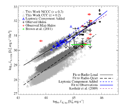
Figure 4: Radio-to-X-ray and radio-to-SZ scaling relations in our extended CR model (see main text for the details of the chosen parameters) compared with observations. Left. $L_{1.4~{}\mathrm{GHz}}-L_{\mathrm{X,bol}}$ relation in comparison to the observational sample taken from the literature and detailed in Appendix D. We additionally show the detected signal of Mpc-scale diffuse emission in a stacked sample of radio-quiet galaxy clusters (green, Brown et al., 2011). Right. $L_{1.4~{}\mathrm{GHz}}-Y_{\mathrm{SZ}}$ relation in comparison with the PSZ(V) sample (direct integration method) of Sommer & Basu (2014) together with the data points shown in their Fig. 13.

5.2.2 Model realization

In order to compare with observations, we select a particular realization of our extended CR model. To this end, we use the MultiDark cluster sample at $z=0.2$, which compares well with the redshift of the observational samples (see above and Appendix D). We divide our cluster sample randomly into radio-quiet and radio-loud clusters, assuming a ratio of 10 per cent of the latter (see next section). In our model, we use the turbulent propagation parameter $\gamma_{\mathrm{tu}}$ to separate both populations. In radio-quiet clusters, we assign $\gamma_{\mathrm{tu}}=1$, and in radio-loud clusters, we adopt randomly and uniformly $\gamma_{\mathrm{tu}}$ values in the intervals $[40,80]$ and $[1,5]$ for NCCCs and CCCs, respectively.

Our modeling of magnetic fields is inspired by Faraday rotation studies that point to higher field values in the core region of CCCs compared to NCCCs (Bonafede et al., 2010; Kuchar & Enßlin, 2011), presumably due to the higher adiabatic compression factor during the formation of the cooling core. Hence, for radio-quiet clusters, we adopt randomly and uniformly distributed values of the central magnetic field $B_{0}$ in the intervals $[2.5,5.5]$ $\mu$G and $[5,10]$ $\mu$G for NCCCs and CCCs, respectively. To account for the potential turbulent dynamo in radio-loud objects (characterized by a higher turbulent transport parameter in our model), we slightly increase $B_{0}$ in those objects and chose $B_{0}$ intervals of $[4.5,7.5]$ $\mu$G and $[7.5,12.5]$ $\mu$G for NCCCs and CCCs, respectively.

We fix $\alpha_{\mathrm{B}}=0.5$ and $g_{\mathrm{CR}}=0.5$ for all clusters. We note that our parameter choices are mostly phenomenologically driven with the aim to reproduce observations. The parameter study in Fig. 3 exemplifies considerable degeneracies so that different combinations of parameters can potentially result in very similar distributions. We emphasize the need of more detailed observations of RHs and in particular of multi-frequency correlation studies to constrain the interplay of some of these parameters.

In Fig. 4, we show our model in comparison to the observed radio-to-X-ray and radio-to-SZ scaling relations. The normalization of our model can be arbitrarily varied by changing $g_{\mathrm{CR}}$ as long as the resulting $X_{\mathrm{CR}}$ respects the current observational constraints and remains below a few percents. As explained above, our choice of $g_{CR}=0.5$ ensures an average CR-to-thermal pressure of 2 per cent within $R_{500}$.

Our model is sufficiently flexible to either mimic a cluster radio bimodality or not, depending on the parameters adopted for the populations of radio-loud and radio-quiet objects. However, with the given model realization as in Fig. 4, the separation of the radio-loud and radio-quiet populations is substantially larger in the $L_{1.4~{}\mathrm{GHz}}-L_{\mathrm{X,bol}}$ plane than in the $L_{1.4~{}\mathrm{GHz}}-Y_{\mathrm{SZ}}$ plane, which exhibits almost a continuum distribution from radio-loud CCCs to the radio-quiet NCCCs. This is mainly because the bolometric X-ray emissivity scales with $\rho_{\mathrm{gas}}^{2}$ while $Y_{\mathrm{SZ}}\propto\rho_{\mathrm{gas}}$ (which is only strictly valid for an isothermal gas distribution). This is one plausible explanation for the observed discrepancy of the presence of a bimodality in $L_{1.4~{}\mathrm{GHz}}-L_{\mathrm{X,bol}}$ and the apparent absence of it in $L_{1.4~{}\mathrm{GHz}}-Y_{\mathrm{SZ}}$.

The slope of our model depends on the different parameter choices and, particularly, on the relative differences introduced for the NCCC/CCC and the radio-loud/quiet populations. However, we note that our $L_{1.4~{}\mathrm{GHz}}-L_{\mathrm{X,bol}}$ and $L_{1.4~{}\mathrm{GHz}}-Y_{\mathrm{SZ}}$ scaling relations are somewhat shallower than the observed relation, more similar to the model by Kushnir et al. (2009). This may hint at the contribution of a second, leptonic component that would steepen the slope of our model scaling relation at high mass. In particular, the finding of Cassano et al. (2013) that clusters do seem to show a bimodality at very high $Y_{\mathrm{SZ}}$ may also be an hint of an increasingly important leptonic component. However, we do not expect this component to significantly alter our conclusions regarding the luminosity functions of the next section for the following reasons. (i) The leptonic component would only be present in the radio-loud merging NCCC sample, i.e., the radio (giant) halos, and (ii) it would only be dominant at very high masses because the dissipated energy that is available for energizing fossil electrons should be a fraction of the thermal energy which scales with cluster mass as $E_{\mathrm{th}}\propto M_{200}^{5/3}$ (Cassano & Brunetti, 2005, for magneto-turbulent re-acceleration models). In fact, our $z=0.2$ mock sample, only contains $31$ radio-loud NCCCs with $M_{200}\geq 5\times 10^{14}~{}h_{70}^{-1}$ M_⊙, which is the mass range of, e.g., turbulently reaccelerated RHs (Cassano et al., 2010).

To visualize such a possible leptonic component, we boost the total flux of these 31 radio-loud NCCCs according to $L_{1.4~{}\mathrm{GHz,boosted}}=L_{1.4~{}\mathrm{GHz,had}}+L_{1.4~{}\mathrm{GHz,boost}}$, where $L_{1.4~{}\mathrm{GHz,had}}$ is the radio luminosity of our extended hadronic component and

$$L_{1.4~{}\mathrm{GHz,boost}}=L_{1.4~{}\mathrm{GHz,had}}\times\left(\frac{M_{500}}{7.5\times 10^{14}~{}h_{70}^{-1}~{}\mathrm{M}_{\odot}}\right)^{2.3}\propto M_{500}^{4}\,.$$ (13)

We consider this to be a phenomenological correction factor that aims at reproducing the observed relation $L_{1.4~{}\mathrm{GHz}}\propto M_{500}^{4}$ (Cassano et al., 2007; Cassano et al., 2013). Possible physical realizations include turbulent re-acceleration of primary or secondary (hadronically produced) electrons (Brunetti & Lazarian, 2011) or re-acceleration of fossil electrons by means of diffusive shock acceleration (Kang & Ryu, 2011; Kang et al., 2012; Pinzke et al., 2013). Here we tie the leptonic component to our modeling of the magnetic field and the hadronic emission component, which provides guidance for the missing signal fraction that we require by our surface brightness modeling. As $L_{1.4~{}\mathrm{GHz,had}}\propto M_{500}^{1.7}$, we adopt an additional mass scaling to reach the desired $L_{1.4~{}\mathrm{GHz}}\propto M_{500}^{4}$. The resulting median (mean) boost is about 32 per cent (47 per cent) of the hadronic component. The boosted population is shown in both panels of Fig. 4. The corresponding scaling relations have slopes close to the ones of the $L_{1.4~{}\mathrm{GHz}}-L_{\mathrm{X,bol}}$ and $L_{1.4~{}\mathrm{GHz}}-Y_{\mathrm{SZ}}$ observational samples, respectively.

At low SZ fluxes, there are a considerable number of radio loud radio mini halos visible in CCCs that fall above the observed $L_{1.4~{}\mathrm{GHz}}-Y_{\mathrm{SZ}}$ relation by Sommer & Basu (2014). However, this does not challenge our model because (i) in order to characterize the radio halo emission, Sommer & Basu (2014) apply a low-pass filter to the radio data, which minimizes any flux contribution from radio mini-halos that are comparable or smaller than the chosen filter size and (ii) the radio mini-halo population in the literature suffers from incompleteness effects (Giacintucci et al., 2014).

Owing to the many uncertainties and lack of robustness both in the observations and modeling at this stage, we do not attempt to fine-tune our model to the observations. In particular, we refrain from introducing any mass-dependence in our free parameters at this stage. Additionally, we do not include the possible leptonic emission component in the analysis of next section, deferring the study of its physical details and correlation to the hadronic component to future work. The mock cluster sample used here is affected by incompleteness in the highest-mass range because of the limited volume of the MultiDark simulation (Paper I). Only a small number of objects that lie in this mass range would be affected by such a correction, as discussed above and shown in Fig. 4. These are not statistically significant in comparison to the RH abundances that we will find in the next section. Interestingly, the detected signal of Mpc-scale diffuse emission in a stacked sample of radio-quiet galaxy clusters (shown in green in the left plot of Fig. 4, Brown et al., 2011) agrees with the expected signal of our radio-quiet population.

6 Luminosity Functions

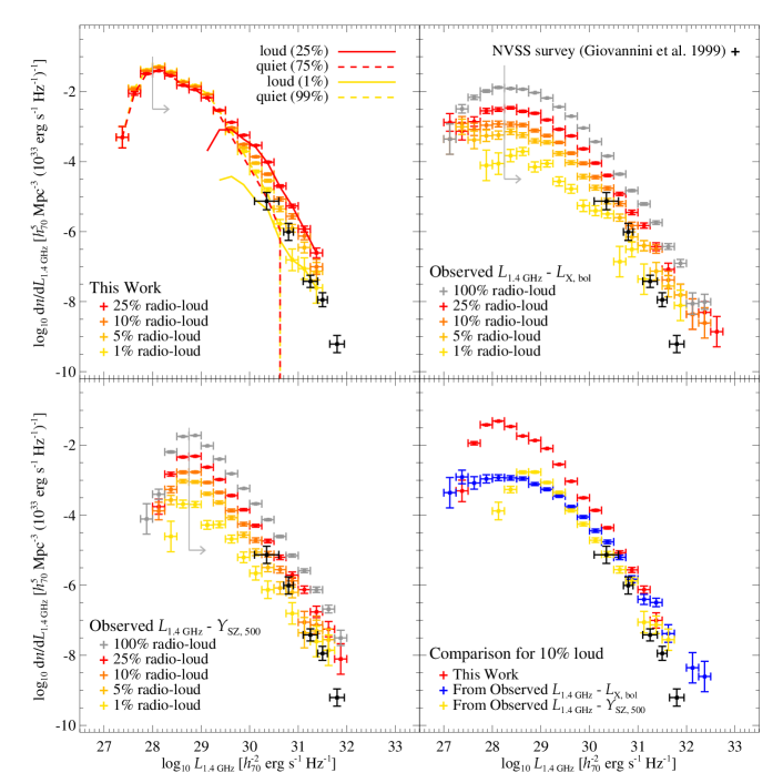
Figure 5: RH luminosity function (RLF) at 1.4 GHz. The top left panel shows the RLF of our extended CR model (see main text for the details of the chosen parameters) for different fractions of radio-loud clusters. Additionally shown is the contribution of radio-quiet and radio-loud populations to the total RLF (assuming a fraction of 25 per cent and 1 per cent of radio-loud objects). The top right panel shows the RLF obtained by applying the observed $L_{1.4~{}\mathrm{GHz}}-L_{\mathrm{X,bol}}$ relation (see left panel of Fig. 4) to the MultiDark clusters at $z=0.2$, using our phenomenological gas model for $L_{\mathrm{X,bol}}$ of each cluster; again for different percentages of radio-loud clusters. The bottom left panel shows the RLF obtained by applying the observed $L_{1.4~{}\mathrm{GHz}}-Y_{\mathrm{SZ},500}$ relation (see right panel of Fig. 4) to the MultiDark clusters at $z=0.2$, using $Y_{\mathrm{SZ},500}$ of our our phenomenological gas model for each cluster. The bottom right panel shows the comparison between the three approaches for 10 per cent of radio-loud clusters. In all panels, we show the NVSS survey RLF (Giovannini et al., 1999) with a median redshift of $z\approx 0.18$, corrected for the sample incompleteness and survey sky coverage. Horizontal error bars represent the mass bins while the vertical error bars are Poissonian uncertainties. The light gray line marked by the arrow estimates the incompleteness limit owing to the adopted low-mass cut (in the construction of the mock cluster catalog, see Paper I) and the scatter in the halo luminosities.

6.1 Comparison with observations at 1.4 GHz

In Fig. 5, we show the RH luminosity function (RLF) at 1.4 GHz for a representative realization of our extended CR model (as in Section 5), and compare it with observational results. The RLF is completely determined by the cluster mass function and the radio luminosity-to-mass relation, through $L_{1.4~{}\mathrm{GHz}}-L_{\mathrm{X,bol}}$ or $L_{1.4~{}\mathrm{GHz}}-Y_{\mathrm{SZ}}$ in combination with our phenomenological gas model (see Paper I). However, in the radio band there is the additional uncertainty of the fraction of radio-loud clusters. Thus, in Fig. 5, we also show the RLFs obtained by applying the observed $L_{1.4~{}\mathrm{GHz}}-L_{\mathrm{X,bol}}$ and $L_{1.4~{}\mathrm{GHz}}-Y_{\mathrm{SZ}}$ relations (as in Fig. 4) to our $z=0.2$ mock catalog, which employs our phenomenological gas model for $L_{\mathrm{X,bol}}$ and $Y_{\mathrm{SZ},500}$ of each cluster, respectively. Note that this procedure is only applied to halos defined as radio-loud clusters (which are by definition accounted for in the $L_{1.4~{}\mathrm{GHz}}$ scaling relations) and we assume a fraction of 1, 0.25, 0.1, 0.05 and 0.01 of radio-loud clusters. As evident from Fig. 5, this differs for our model scaling relations: there we also define a fraction of radio-loud clusters, but the radio-quiet population also contributes to the RLF with an increasing fraction at low luminosities. This is exemplified in the top left plot of Fig. 5, which shows the contribution of radio-quiet and loud populations to the total RLF, assuming a fraction of 0.25 and 0.01 of radio-loud objects.

In Appendix D, we make an attempt to construct an RLF from existing X-ray flux-limited radio surveys. Of the few existing studies, we select the cluster radio survey done with the National Radio Astronomy Observatory (NRAO) Very Large Array (VLA) sky survey (NVSS) at $1.4$ GHz of Giovannini et al. (1999) and the survey with the Giant Metrewave Radio Telescope (GMRT) at $610$ MHz by Venturi et al. (2007, 2008). For the latter, we can also construct an RLF at 1.4 GHz using the corresponding RH follow-up measurements. The fractions of radio-loud clusters are about 0.06, 0.18 and 0.24 for the NVSS 1.4 GHz, GMRT 610 MHz and GMRT 1.4 GHz samples, respectively. As explained in Appendix D, we use the 1.4 GHz NVSS RLF (with a median redshift of $z\approx 0.18$) as observational reference for our comparisons. We conclude that the observational determinations of the RLF is not very robust at this stage; the very different fractions of radio-loud clusters found in the different studies is one indicator of this. Recently, Kale et al. (2013) found only one additional radio mini-halo in an extended GMRT survey. This does not significantly increase the statistics of RLF studies with respect to the sample of Venturi et al. (2007, 2008). We therefore decided to keep the 1.4 GHz NVSS RLF as our observational reference.

Generally, there is fair agreement between the NVSS RLF and both our modeled RLF and the RLFs based on observational scaling relations, particularly for radio-loud fractions between 10 per cent and 1 per cent. In particular, we verified that the cumulative number of RHs above a certain flux limit of the NVSS survey is well matched by the case of a radio-loud fraction of 10 per cent, which will be used in the following section. The RLF obtained from the $L_{1.4~{}\mathrm{GHz}}-L_{\mathrm{X,bol}}$ relation differs from the NVSS RLF at high luminosities, presumably caused by the large observed scatter. On the other side, the RLF obtained from the $L_{1.4~{}\mathrm{GHz}}-Y_{\mathrm{SZ}}$ relation matches the NVSS result better. These results need to be consolidated by RLFs corrected for flux-incompleteness and simulations of larger cosmological volumes that are more complete at the high-mass end. Figure 5 demonstrates that it will be difficult to discriminate between different scenarios at high radio luminosities (or equivalently masses). Indeed, in the bottom right panel of Fig. 5 we compare our RLF and the RLFs based on observational scaling relations for a 10 per cent fraction of radio-loud clusters to the NVSS RLF. This suggests that the low-luminosity (low-mass) clusters will be the most useful in disentangling between different models. This emphasizes the importance of conducting homogeneous, well controlled surveys of RHs with the Jansky VLA, ASKAP (Norris et al., 2011) and APERTIF (Röttgering et al., 2012) at 1.4 GHz and LOFAR at lower frequencies. Since the latter has already started to take data, it is extremely timely to present RLF predictions in this wavelength regime for our extended hadronic model, which we will do next.

6.2 Low-frequency predictions at 120 MHz

In Fig. 6, we show our model predictions at 120 MHz obtained with the same representative realization of our model as in Section 5, with 10 per cent radio-loud clusters at all redshifts. We show both the differential RLF (top left panel) and the cumulative number density (bottom left panel) at different redshifts (corresponding to different the MultiDark snapshots in Table 1 of Paper I). We note that the redshift evolution is almost entirely due to the $B^{2}/(B^{2}+B_{\mathrm{CMB}}^{2})$ factor of equation (18) since $B_{\mathrm{CMB}}\propto(1+z)^{2}$. Our imposed mass cutoff of $M_{200}=10^{14}\,h^{-1}\,M_{\odot}$, which has been adopted to reliably model the cluster gas distribution (Paper I), translates into a luminosity cutoff. This causes the differential luminosity function to turn over at the low-luminosity end and artificially flattens the slope already at sightly higher luminosities than the luminosity maximum that indicates our formal incompleteness limit. Note that calibrating our model to 1.4 GHz observations may cause an over- or underestimate of the number of low-frequency halos as a result of intrinsic spectral flattening towards low frequencies (e.g., due to CR transport) or steeper leptonic spectra in comparison to the hadronic component in the high-mass radio-loud NCCC population, respectively.

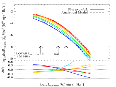
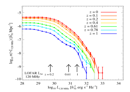
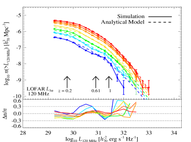
Figure 6: RH luminosity function $n(L,z)$ at 120 MHz (top left panel) and cumulative number density of RHs $n(>L,z)$ (bottom left panel) at different redshifts $z$ (color coded) for the model realization described in Section 5 with a 10 per cent fraction of radio-loud clusters. To obtain an analytical model for $n(L,z)$, we fit the logarithm of the RLF at each $z$ with a second-order polynomial and constrain the evolution of the three free parameters to follow a linear function in $1+z$ (see main text for details). The right panels show the comparison of the RLF fits (top) and the cumulative number density of the MultiDark samples (bottom) to the constrained analytical model. The bottom panels on the right-hand side show the relative differences $\Delta n/n=(n_{\mathrm{analytical}}-n_{\mathrm{fit}})/n_{\mathrm{fit}}$ (top) and $\Delta n/n=(n_{\mathrm{analytical}}-n_{\mathrm{simulation}})/n_{\mathrm{simulation}}$ (bottom). Additionally shown is the LOFAR Tier 1 point-source flux limit of $F_{5\sigma}^{\mathrm{PS}}=0.5$ mJy (Röttgering et al., 2012) converted to a luminosity limit at a given redshift. Horizontal error bars represent the mass bins while the vertical error bars are Poissonian uncertainties. The light gray line marked by the arrow estimates the incompleteness limit owing to the adopted low-mass cut (in the construction of the mock cluster catalog, see Paper I) and the scatter in the halo luminosities.

Additionally shown in Fig. 6 is the expected LOFAR Tier 1 point-source flux limit of $F_{5\sigma}^{\mathrm{PS}}=0.5$ mJy (Röttgering et al., 2012) converted to a luminosity limit at a few representative redshifts. This flux limit is clearly an underestimate for nearby RHs, which extend over angular scales $\sim 1$ deg, as e.g., in the case of the Coma radio halo. In order to make more reliable predictions, we will calculate the RH flux limit with equation (10) of Cassano et al. (2010) that is based on the assumption that RHs emit about half of their total radio flux within their half radius. In our sample, the typical radius within which half of the radio flux is emitted is $R_{500}/4$, and we require that the flux within this radius is higher than $F_{5\sigma}^{\mathrm{PS}}$. The median $R_{500}$ of our sample is about $0.8$ $h_{70}^{-1}$ Mpc at all redshifts. This translates to a flux limit of about $48,14,3.5$ and $2.5$ mJy at $z=0.1,0.2,0.6$ and $1$, respectively.

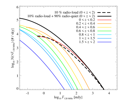
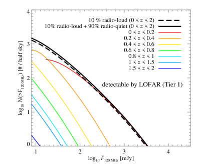
Figure 7: Cumulative number of RHs above a certain flux limit in an all-sky survey at 120 MHz. We show the result of the model realization described in Section 5 using all clusters and adopting a fraction of 10 per cent of radio-loud clusters (black solid line). Additionally, we show the result obtained by using the 10 per cent radio-loud clusters only (black dashed line). We also show the differential contribution to the RLF in redshift slices. Note that the number of (detectable) RHs would be dramatically reduced by the presence of a break in the model at some low luminosity-scale, or a mass-dependence of the model parameters causing the RH luminosities to decrease at low masses. Left. Total number of RHs in the sky. Right. Number of detectable RHs by the LOFAR Tier 1 survey considering its sky coverage (half sky) and adopting a realistic flux limit corresponding to different angular source extensions at different redshifts (see main text for details).

To derive low-frequency flux functions, we construct an analytical model for the evolving RLF. We fit the 120 MHz RLF at different redshifts with a second-order polynomial of the form $\log_{10}\mathrm{d}n/\mathrm{d}L_{120~{}\mathrm{MHz}}=A_{0}+A_{1}~{}\log_{10}L_{120~{}\mathrm{MHz}}+A_{2}~{}(\log_{10}L_{120~{}\mathrm{MHz}})^{2}$. All luminosities are measured in units of $h_{70}^{-2}\mathrm{erg~{}s}^{-1}\,\mathrm{Hz}^{-1}$ and (comoving) number densities in units of $h_{70}^{3}\,\mathrm{Mpc}^{-3}$. We consider only luminosities with $\log_{10}L_{120~{}\mathrm{MHz}}\geq 29.25$ to exclude the turn-over at low luminosities caused by incompleteness. To obtain an analytical model for $n(L,z)$, we constrain the evolution of the three free parameters $A_{i}$ to follow a linear function in $1+z$, i.e., $A_{i}=A_{i,0}+A_{i,1}~{}(1+z)$. In the right panels of Fig. 6, we compare the RLF fits (top) and the cumulative number density in the simulation (bottom) to the analytical model. In particular the analytics matches the simulation well except for high luminosities and high redshifts where small number statistics explains the deviations.

This analytical model describes the number of RHs expected in our model per unit luminosity and per unit comoving volume $V_{\mathrm{c}}$, i.e., $\mathrm{d}^{2}N(L,z)/\mathrm{d}V_{\mathrm{c}}\mathrm{d}L$. Hence the cumulative number of RHs above a given flux limit $F$ is given by the integral

$$N(>F)=\int_{z_{1}}^{z_{2}}\int_{L(F)}^{\infty}\frac{\mathrm{d}^{2}N(L,z)}{\mathrm{d}V_{\mathrm{c}}\mathrm{d}L}\,\frac{\mathrm{d}V_{\mathrm{c}}}{\mathrm{d}z}\,\mathrm{d}z\,\mathrm{d}L,$$ (14)

where $L(F)=4\pi D(z)^{2}F$ and $D(z)$ is the luminosity distance to an RH at redshift $z$. The result is shown in the left panel of Fig. 7 for the model realization described in Section 5 with a 10 per cent fraction of radio-loud clusters (black solid line). We limit the integral to luminosities $\log_{10}L_{120~{}\mathrm{MHz}}\geq 29.25$. Our redshift integration extends from $z_{1}=0.018$, the redshift of the closest known RH in Perseus, to $z_{2}=2$. As shown in Fig. 7, already redshifts $z\gtrsim 1$ do not significantly contribute to the flux function. Additionally, there are large theoretical uncertainties since our gas model is not calibrated for these redshifts (and implied low-mass range) and very little is observationally known about diffuse radio emission on group scales in particularly at these redshifts, which motivates our upper redshift limit. Note also that at these high redshifts, the analytical fit to the evolving RLF slightly overproduces the simulation number counts.

Figure 7 shows the contribution of different redshift slices to the total flux function. We contrast this to the flux function using only the subsample of 10 per cent radio-loud clusters (black dashed line). This was obtained by constructing the corresponding RLF and repeating the steps above in building an analytical model, however, discarding luminosities $\log_{10}L_{120~{}\mathrm{MHz}}\leq 30.75$ in the integration.

In the right panel of Fig. 7, we show the total number of RHs that would be detectable by the LOFAR Tier 1 survey, where its sky coverage (of about half the entire sky) and the signal degradation due to source extensions of close-by RHs is taken into account. The latter is calculated with equation (14) and adopting $F=F_{\mathrm{min}}$ where $F_{\mathrm{min}}$ is given by equation (10) of Cassano et al. (2010) as explained above. Comparing the left and right panel of Fig. 7 elucidates the critical impact of the detection threshold on the number observable RHs. A detailed characterization of the instrumental response is needed in order to obtain more precise estimations.

The LOFAR Tier 1 survey at 120 MHz should be able to detect about $1400$ clusters hosting radio giant and mini halos, considering the hadronic component only. We refer the reader to Cassano et al. (2010) for predictions for giant halos in the turbulent re-acceleration scenario. We note that those are complementary, because they address a larger mass scale with respect to ours, which are limited by the volume of the MultiDark simulation (see Paper I).

The precise number of detections depends strongly on the underlying assumptions. There are two main uncertainties in our model: the fraction of radio-loud to radio-quiet clusters and the corresponding luminosities as well as our assumed RH modeling in low-mass clusters (which are not yet known to host RHs). The fraction of radio-loud to radio-quiet clusters is determined from a given (degenerate) set of model parameters that include $\gamma_{\mathrm{th}}$, $B_{0}$, $\alpha_{B}$, $g_{\mathrm{CR}}$, or equivalently $X_{CR}$. The fraction of radio-loud clusters mostly affects the number of medium-to-high luminosity RHs (as can be seen from the 1.4 GHz RLFs in the top left panel of Fig. 5). The total number of RHs is dominated by low-luminosity RHs. While this may suggest that the radio-loud fraction is of minor importance for the number of detectable RHs, the opposite is the case. Because of the flux limit, only the most luminous clusters at each redshift are observable so that the total number of detectable RHs scales almost linearly with the radio-loud fraction.

We caution that our predicted total number of (detectable) RHs depends on the ability to extrapolate the observed and modeled scalings down to our adopted mass limit of $M_{200}\approx 1.4\times 10^{14}$ $h_{70}^{-1}$ M_⊙. If the underlying physics imprinted a characteristic scale into the CR transport or magnetic field distribution, this would manifest itself as a break in the radio luminosity scaling relations and dramatically reduce (or even increase) the number of expected RHs. While this does not interfere with previous (high-frequency) measurements at high luminosities, this may of critical importance for future, more sensitive (low-frequency) measurements of low-redshift clusters that probe the uncertain regime of diffuse radio emission in low-mass clusters.

The reason for this lies in the steep halo mass function which ensures that that clusters above a given cutoff (which is either physically motivated or observationally realized through a survey flux limit) dominate the total number of (detectable) RHs. Only if the radio luminosity scaling remains unaltered below the survey flux limit, the steepness of the mass function ensures that there will be more RHs scattered above the flux limit then below it. This is the so-called Eddington bias that causes the inferred luminosities based on only the detected sources to end up as an overestimate. Hence the presence of any hypothetical break in the radio luminosity scaling, which is unconstrained by current data, explains the largely varying model predictions in the recent literature, which vary from a few to hundreds observable RHs (Cassano et al., 2010; Cassano et al., 2012; Sutter & Ricker, 2012) to thousands of detectable RHs in future surveys (Enßlin & Röttgering, 2002).

Another relevant issue in such surveys is the identification of RHs and their hosting clusters (see also Cassano et al., 2010). RHs constitute a small part of the entire (diffuse as well as apparent point-like) radio source population and therefore need to be distinguished from the emission produced by other sources. A good approach will be to cross-correlate the radio maps with high-sensitivity X-ray surveys such as that by the future eROSITA mission, which is expected to detect around $10^{5}$ clusters up to redshift $z\approx 1.3$ (e.g., Cappelluti et al., 2011).

Our results show the prospects of the LOFAR survey and other future radio instruments in determining the RH properties over a broad range of luminosities. This should permit a robust determination of the number of clusters hosting RHs at a given luminosity (mass) and to carefully asses completeness issues. This will be extremely helpful in elucidating the RH generation mechanism, in determining the viable parameter space for the hadronic model and in establishing the precise role of the hadronic contribution to the total radio emission of merging clusters. In particular, the comparison with the predictions of the turbulent re-acceleration scenario by Cassano et al. (2010); Cassano et al. (2012), where a significantly smaller number of objects is expected to be detected, will eventually help in disentangling different models and in identifying the importance of the hadronic component.

7 Conclusions

This paper aims at scrutinizing the hadronic model for giant and mini radio halos. Our phenomenological modeling of the CR distribution is guided by cosmological cluster simulations and theoretical considerations of microscopic CR transport. It is designed to efficiently and simultaneously model the RH surface brightness emission, RH scaling relations and luminosity functions. Within the hadronic scenario, the interplay of CR advection and streaming appears to be crucial to match observed RH distributions as a function of SZ flux as well as to explain the bimodality of radio-loud and radio-quiet clusters at a fixed X-ray luminosity. However, the spatial extend of giant radio halos is difficult to accomplish within the hadronic framework, especially for the Coma halo at low frequencies (Brunetti et al., 2012). This calls for a revision of purely hadronic models for giant radio halos.

To construct an extended model for the CR distribution in clusters, we adopt the universal spatial and spectral CR distribution found in hydrodynamic cosmological simulations of cluster formation (Pinzke & Pfrommer, 2010). Since these simulations only follow the macroscopic, advective CR transport, we additionally account for microscopic CR transport processes (Enßlin et al., 2011; Wiener et al., 2013). While turbulently-driven CR advection can lead to centrally enhanced CR profiles, CR propagation in the form of CR streaming and diffusion produces flatter CR profiles, which should be realized for decaying cluster turbulence. In our model, we introduce a CR propagation parameter $\gamma_{\mathrm{tu}}$ that is the ratio of the CR streaming-to-advection time scale. This parameter allows us to effectively switch the regimes where either process dominates the CR transport and to explore different turbulent states of clusters.

This enables us to model the radio surface brightness profiles of giant radio halos (as exemplified in Coma and Abell 2163) as well as of radio mini-halos (in Perseus and Ophiuchus) at 1.4 GHz. We find an excellent match to mini halos over a wide range of parameter choices, rendering the hadronic model as an attractive explanation for mini halos. However, in order to match the extended surface brightness profiles of giant halos at high frequencies (1.4 GHz), the hadronic model would require flat CR profiles for magnetic field configurations favored by Faraday rotation measurements. These flat CR profiles should only be realized through CR streaming transport in relaxed clusters, which appears to be in conflict with the observation that giant radio halos are hosted by merging turbulent clusters. Moreover, the hadronic model fails to explain the emission in the outer parts of the Coma halo at 352 MHz where not even the extreme case of a flat CR profile is sufficient to explain the emission as of purely hadronic origin. This motivates us to suggest the following new hybrid hadronic-leptonic scenario.

1. Radio mini halos are primarily of hadronic origin.

2. Giant radio halos experience a transition from the central hadronic emission component to a dominantly leptonic emission component in the outer halo that is due to Fermi I or II re-acceleration of fossil or hadronically produced electrons.

3. Steep spectrum radio sources are mainly of leptonic origin.

This scenario would imply an increased spectral and morphological variability in leptonically dominated emission regions because of the intermittency and relative inefficiency of the corresponding re-acceleration processes (Fermi I acceleration at weak intra-cluster shocks or Fermi II acceleration at plasma waves). In particular, it implies a spectral steepening from the hadronic to the leptonic component, since the long-lived CR protons are dominantly accelerated by stronger formation shocks during the gas assembling history onto a cluster, which causes a harder spectrum in comparison to the softer leptonic component. We checked that for parameter ranges that provide acceptable matches to the radio profiles, the resulting gamma-ray emission from the decay of neutral pions—an inevitable by-product in hadronic CR interactions—is below observational gamma-ray upper limits provided by Fermi and imaging atmospheric Cherenkov telescopes.

To address the hadronic RH statistics, we apply our extended CR model to a cosmologically complete mock cluster catalog built from the MultiDark $N$-body simulation in a companion paper (Paper I). We select a representative realization of our extended CR model and compare it with existing radio scaling relations. Because of CR transport and the different gas-density scalings of the X-ray luminosity, $L_{\mathrm{X}}\propto\int\rho_{\mathrm{gas}}^{2}\mathrm{d}V$, and the Sunyaev-Zel’dovich flux, $Y\propto\int\rho_{\mathrm{gas}}k_{\mathrm{B}}T\mathrm{d}V$, our model is able to simultaneously reproduce the observed bimodality of radio-loud and radio-quiet clusters at the same $L_{\mathrm{X}}$ as well as the unimodal distribution of radio-halo luminosity versus $Y$; thereby suggesting a physical solution to this apparent contradiction. We caution however, that some parameters in our model are degenerate with respect to the resulting radio luminosity and radio emission profiles, in particular $\gamma_{\mathrm{tu}}$ and $\alpha_{\mathrm{B}}$ (our rate of decline of the magnetic field toward the cluster outskirts). Multi-frequency data will be needed to better constrain these parameters and to break these degeneracies.

Assuming a redshift-independent fraction of 10 per cent radio-loud clusters, we demonstrate that our model matches the NVSS RH luminosity function (RLF). However, the high-luminosity tail of our model RLF is subject to cosmic variance because of the comparably small simulation volume of $1~{}h^{-3}\,\mathrm{Gpc}^{3}$. Interestingly, the RLF derived from the $L_{1.4~{}\mathrm{GHz}}-L_{\mathrm{X,bol}}$ relation differs at high radio luminosities from the NVSS RLF; possibly because of selection and incompleteness effects that are not fully taken into account. The comparison between different RLFs suggests that the low-luminosity (low-mass) regime is the most promising place to differentiate between various models.

It is expected that the next-generation of low-frequency radio surveys will probe this regime. Hence, we we make prediction for the LOFAR cluster survey, in particular, we compute the 120 MHz RLF and the cumulative RH number density. Given our assumptions, we would expect the LOFAR Tier 1 survey at 120 MHz to detect about $1400\times(\mathrm{\emph{radio-loud~{}fraction}/0.1})$ hadronically-generated radio giant and mini halos. We caution that the precise number depends strongly on the underling assumptions. In particular, we assume that the model parameters can be extrapolated down to cluster masses of about $M_{200}\approx 1.4\times 10^{14}$ $h_{70}^{-1}$ M_⊙ without any break in the radio scaling relation that would indicate additional scales in the physics. Most of the RHs in our sample lie at low masses and thus at low luminosities that are unconstrained by current observations. If, e.g., the magnetic field and/or the CR distribution in clusters are not statistically self-similar and would exhibit much reduced strength/number density on group scales, our predictions for the detectable number of RHs would be dramatically reduced.

This demonstrates the potential of LOFAR, and other next-generation high-sensitivity radio instruments such as APERTIF, ASKAP, EVLA and SKA, in determining the RLF properties. In combination with future X-ray missions like eROSITA, this should yield a robust determination of the number of clusters hosting RHs at a given luminosity (mass) and thus elucidate the relation of the radio emission with the dynamical state of a cluster. This is crucial in order to understand the RH generation mechanism and to establish the precise role of the hadronic contribution in clusters.

We have constructed a model for the ICM (in Paper I) and CR distributions in galaxy clusters that enables us to provide a cosmologically complete multi-frequency mock catalog for the (non-)thermal cluster emission at different redshifts. We make these catalogs publicly and freely available on-line through the MultiDark database (www.multidark.org, Riebe et al., 2013). We hope that the community can make valuable use of these catalogues in synergy with the future radio, X-ray and gamma-ray data.

Appendix A Cosmic Ray Modeling

Here, we describe in detail how our extended model for the CR distribution in galaxy clusters of Section 2 is constructed by generalizing the analytical results by Enßlin et al. (2011).

As anticipated in Section 2, when advection dominates the CR transport, the CR normalization can be expressed as in equation (2). However, when CR streaming and diffusion dominates, the CR distribution is modified and flattens considerably. This can be shown analytically by solving the continuity equation for CRs and obtaining the CR density profile, $\rho_{\mathrm{CR}}$, of equation (3). Assuming $P_{\mathrm{th}}(R)/P_{\mathrm{th},0}=n_{\mathrm{e}}(R)/n_{0}$, i.e., neglecting the temperature dependence, and adopting a standard $\beta$-profile for the electron density,

$$n_{\mathrm{e}}=n_{0}\left(1+\frac{R^{2}}{R_{\mathrm{c}}^{2}}\right)^{-\frac{3\beta_{\mathrm{cl}}}{2}}\,,$$ (15)

Enßlin et al. (2011) find that the solution of equation (3) is physical only for $\rho_{\mathrm{CR}}$ within the radial range $R_{-}<R<R_{+}$ with

$$R_{\pm}=\frac{3\beta_{\mathrm{cl}}}{2\gamma}R_{*}\left(1\pm\sqrt{1-\left(\frac{2R_{\mathrm{c}}\gamma}{3\beta_{\mathrm{cl}}R_{*}}\right)^{2}}\right)\,;$$ (16)

while it is non-stationary outside these radii. In these regions, the authors suggest to set $\rho_{\mathrm{CR}}(R)=\rho_{\rm{CR}}(R_{\pm})$ for $R>R_{+}$ and $R<R_{-}$, respectively. Enßlin et al. (2011) obtain the profile for the CR normalization, $C(R)=C_{0}(\rho_{\mathrm{CR}}(R)/\rho_{\mathrm{CR},0})^{\beta_{\mathrm{CR}}}$, as

$$C(R)=C_{0}\left(1+\frac{R^{2}}{R_{C}^{2}}\right)^{-\beta_{\mathrm{c}}}\mathrm{exp}\left({\frac{R}{R_{*}}\beta_{\mathrm{CR}}}\right)$$ (17)

for $R_{-}<R<R_{+}$, where $\beta_{\mathrm{c}}=3\beta_{\mathrm{cl}}~{}\beta_{\mathrm{CR}}/2\gamma$, and $C(R)=C(R_{\pm})$ for $R<R_{-}$ and $R>R_{+}$, respectively. In this way, different CR transport cases are parametrized through $\gamma_{\mathrm{tu}}$. A high value of $\gamma_{\mathrm{tu}}$ characterizes the advection-dominated case, while the CR profile is flat for $\gamma_{\mathrm{tu}}\sim 1$. We refer the reader to Enßlin et al. (2011) for an extensive discussion.

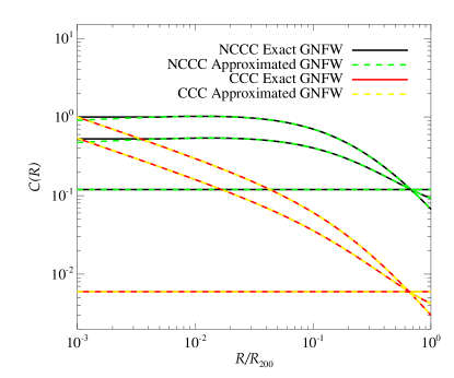
Figure 8: Comparison of the exact and approximate solutions for $C(R)$ in the case of our GNFW profile. In the latter case, we use the formulae by Enßlin et al. (2011) but adopt $P(R)/P_{0}=n_{\mathrm{e,GNFW}}(R)/n_{0}$ for this comparison only, i.e., we assume here an isothermal ICM. We show the GNFW profiles for NCCCs and CCCs, as derived in Paper I. For each of these profile classes, we show three different cases of $\gamma_{\mathrm{tu}}=100$, 10, and 1 (top to bottom). We normalize $C(R)$ for the advection dominated case ($\gamma_{\mathrm{tu}}=100$) at $R=10^{-3}R_{200}$ and and require CR number conservation during CR streaming. Note that the value for $C(10^{-3}R_{200},\gamma_{\mathrm{tu}}=100)$ in the CCC case is identical for the exact solution and its approximation, while there is a small difference of about 9 per cent in the NCCC case. We adopt $\alpha=2.3$.

We want to extend this result to account for (i) our GNFW gas profiles of Paper I, (ii) the universal temperature drop in the cluster outskirts, and (iii) merge it with the universal cluster mass-scaling of the CR normalization, $\tilde{C}$, obtained from hydrodynamical simulations (Pinzke & Pfrommer, 2010). Therefore, we adopt the extended profile, $C_{\rm{extended}}=\tilde{C}(R)(\rho_{\mathrm{gas}}(R)/m_{\mathrm{p}})(T(R)/T_{0})$, of equation (5). We note that for such a choice, there does not any more exist an analytical solution to equation (3) as in Enßlin et al. (2011). This results in a 5-order equation and a numerical solution would not be of practical use for every cluster in our large MultiDark sample. For simplicity, we adopt the formulae above also for our extended model. I.e., we adopt $C(R)=C_{0}(\rho_{\mathrm{CR}}(R)/\rho_{\mathrm{CR},0})^{\beta_{\mathrm{CR}}}$ within $R_{\pm}$ of equation (16), with $\rho_{\mathrm{CR}}$ defined by equation (3) where $C_{\mathrm{extended}}$ enters through the advective CR profile, $\eta(R)$, of equation (4), and $C(R)=C(R_{\pm})$ for $R>R_{+}$ and $R<R_{-}$, respectively. Note that, in our formalism, $R_{\mathrm{c}}$ of equation (16) becomes the characteristic radius of our GNFW gas profile (see Paper I), i.e., $R_{\mathrm{c}}=0.2R_{500}$, and $\beta_{\mathrm{cl}}=0.8$ (we checked that varying the value of $\beta_{\mathrm{cl}}$ between 0.4 and 1.2 has no impact). The relevant factors are $\gamma_{\mathrm{tu}}$ and the exponential factor of equation (3). As we will see in the following, the two radii $R_{\pm}$ are not critically affected by the form of $\eta(R)$. Therefore, despite the approximation, this approach captures the main CR transport effects.

Assuming our GNFW gas profile instead of a standard $\beta$-profile for the electron density, so adopting $P(R)/P_{0}=n_{\mathrm{e,GNFW}}(R)/n_{0}$, there exist an exact analytical solution to equation (3) as in Enßlin et al. (2011). In order to evaluate the systematic error that we are introducing with the approach described above, in Fig. 8, we compare the exact solution for $C(R)$ in the case of our GNFW profile with the approximate solution where we use the formulae by Enßlin et al. (2011), and only substitute the electron $\beta$-profile for our GNFW profiles (with $R_{\mathrm{c}}=0.2R_{500}$, $\beta_{\mathrm{cl}}=0.8$). In this last case, we fix $R_{-}=10^{-3}R/R_{200}$ to mimic the typical $R_{-}$ value of the exact solution, otherwise an unphysical step feature would appear at $\leq 10^{-2}R/R_{200}$. This latter approximation is kept in our extended model, which however has no impact on the model surface brightness and total luminosity. There is almost no difference between the two cases, as clear from Fig. 8. This shows that the approach presented here to construct our extended model can be safely followed in order to derive a fully working parametrization which captures the main CR transport effects.

Appendix B Radio Emission

The synchrotron emissivity $j_{\nu}$, at frequency $\nu$ and per steradian, of a steady-state electron population where radiative cooling balances injection from hadronic interactions (adapted from Pfrommer et al., 2008 and Enßlin et al., 2011) is given by

$$j_{\nu}=A_{\nu}C(R)\rho_{\mathrm{gas}}(R)\frac{\epsilon_{\mathrm{B}}(R)}{\epsilon_{\mathrm{B}}(R)+\epsilon_{\mathrm{CMB}}}\left(\frac{\epsilon_{\mathrm{B}}(R)}{\epsilon_{B_{\mathrm{c}}}}\right)^{(\alpha-2)/4}\,,$$ (18)

where $\epsilon_{\mathrm{CMB}}$ is the energy density of the cosmic microwave background (CMB), $\epsilon_{B}=B^{2}/(8\pi)$ denotes the magnetic energy density, and $B_{\mathrm{c}}=\sqrt{8\pi\epsilon_{B_{\mathrm{c}}}}\simeq 31\left(\nu/\mathrm{GHz}\right)~{}\mu$G. The factor $A_{\nu}$ is given by:

$$A_{\nu}=A_{\mathrm{E_{synch}}}\frac{16^{2-\alpha_{\mathrm{e}}}\sigma_{\mathrm{pp}}m_{\mathrm{e}}c^{2}}{(\alpha_{\mathrm{e}}-2)\sigma_{\mathrm{T}}\epsilon_{B_{\mathrm{C}}}m_{\mathrm{p}}}\left(\frac{m_{\mathrm{p}}}{m_{\mathrm{e}}}\right)^{\alpha_{\mathrm{e}}-2}\left(\frac{m_{\mathrm{e}}c^{2}}{\mathrm{GeV}}\right)^{\alpha_{\mathrm{e}}-1}\,,$$ (19)

with

$$A_{\mathrm{E_{synch}}}=\frac{\sqrt{3\pi}}{32\pi}\frac{B_{\mathrm{c}}e^{3}}{m_{\mathrm{e}}c^{2}}\frac{\alpha_{\mathrm{e}}+\frac{7}{3}}{\alpha_{\mathrm{e}}+1}\frac{\Gamma\left(\frac{3\alpha_{\mathrm{e}}-1}{12}\right)\Gamma\left(\frac{3\alpha_{\mathrm{e}}+7}{12}\right)\Gamma\left(\frac{\alpha_{\mathrm{e}}+5}{4}\right)}{\Gamma\left(\frac{\alpha_{\mathrm{e}}+7}{4}\right)}\,,$$ (20)

where $\alpha_{\mathrm{e}}=\alpha+1$, the effective inelastic cross-section for proton-proton interactions is $\sigma_{\mathrm{pp}}=32~{}(0.96+\mathrm{e}^{4.42-2.4\alpha})$, and $\Gamma$ is the Gamma-function (Abramowitz & Stegun, 1965). $A_{\mathrm{E_{synch}}}$ is given in units of erg, and $A_{\nu}$ is given in units of erg cm³ g^-1 sr^-1.

The generalization of the radio emissivity, $j_{\nu}$, to account for three CR populations, each characterized by different power-law spectra and the inclusion of the normalization parameter $g_{\mathrm{CR}}$, following Pinzke & Pfrommer (2010), is straight forward. We obtain

$$j_{\nu,\mathrm{extended}} = g_{\mathrm{CR}}C(R)\rho_{\mathrm{gas}}(R)\frac{\epsilon_{\mathrm{B}}(R)}{\epsilon_{\mathrm{B}}(R)+\epsilon_{\mathrm{CMB}}}$$ (21)

$$\times \Sigma_{i=1}^{3}\Delta_{i}A_{\nu,i}\left(\frac{\epsilon_{\mathrm{B}}(R)}{\epsilon_{B_{\mathrm{c}}}}\right)^{\frac{\alpha_{i}-2}{4}}\,,$$

where the sum is over the three CR spectral indexes $\alpha_{i}=(2.55,2.3,2.15)$ with the corresponding factors $\Delta_{i}=(0.767,0.143,0.0975)$ found by Pinzke & Pfrommer (2010).

Appendix C Gamma-ray Emission

The gamma-ray flux above an energy $E_{\gamma}$ is given by (e.g., Pinzke & Pfrommer, 2010)

$$F_{\gamma}(>E_{\gamma})=\frac{1}{4\pi D^{2}}\int dV\lambda_{\gamma}(R)\,,$$ (22)

where the omnidirectional (i.e., integrated over the $4\pi$ solid angle) gamma-ray emissivity above $E_{\gamma}$ is $\lambda_{\gamma}(R)=A_{\gamma}C(R)\rho_{\mathrm{gas}}(R)$. The parameter $A_{\gamma}$ is (Pinzke & Pfrommer, 2010)

$$A_{\gamma}=g_{\mathrm{CR}}D_{\gamma,\mathrm{break}}\frac{4m_{\pi^{0}}c}{3m_{\mathrm{p}}^{2}}\Sigma_{i=1}^{3}\Delta_{i}\frac{\sigma_{\mathrm{pp},i}}{\alpha_{i}\delta_{i}}\left(\frac{m_{\mathrm{p}}}{2m_{\pi^{0}}}\right)^{\alpha_{i}}\times$$

$$\times\left[\beta_{x}\left(\frac{\alpha_{i}+1}{2\delta_{i}},\frac{\alpha_{i}-1}{2\delta_{i}}\right)\right]_{x_{1}}^{x_{2}}\,,$$ (23)

where $x_{j}=\{1+[m_{\pi^{0}}c^{2}/(2E_{\gamma,j})]^{2\sigma_{i}}\}$, $\left[\beta_{x}(a,b)\right]_{x_{1}}^{x_{2}}=\beta_{x_{2}}(a,b)-\beta_{x_{1}}(a,b)$ where $\beta$ denotes the incomplete Beta-function (Abramowitz & Stegun, 1965), and $\delta_{i}=0.14\alpha_{i}^{-1.6}+0.44$. The term $D_{\gamma,\mathrm{break}}=D_{\gamma}(E_{\gamma},E_{\gamma,\mathrm{break}})$ represents diffusive CR losses due to escaping protons from the cluster at the equivalent photon energy for the break $E_{\gamma,\mathrm{break}}$ (see Pinzke & Pfrommer, 2010 for details). $A_{\gamma}$ is given in units of cm³ s^-1 g^-1.

Appendix D Observational Radio-to-X-ray Scaling relation and Luminosity Function

For comparison with the observed 1.4 GHz radio-to-X-ray scaling relation, we include almost all RHs of the sample by Enßlin et al. (2011). We exclude RXCJ1314.4-2515 and Z7160 because they lack bolometric X-ray measurements. We add to our sample the clusters Ophiuchus, A2029 and A1835 (Govoni et al., 2009). The bolometric X-ray luminosities, $L_{\mathrm{X,bol}}$, of clusters hosting giant radio halos are taken from Brunetti et al. (2009), while $L_{\mathrm{X,bol}}$ values of cluster hosting for mini-halos are taken from Reiprich & Böhringer (2002), Boehringer et al. (1998) and ACCEPT. In the cases where measurement uncertainties for X-ray and radio luminosities are not reported, we adopt a 10 per cent uncertainty. Our final RH sample has a median redshift of $z\approx 0.18$. In the left panel of Fig. 4, we show the corresponding radio-to-X-ray scaling relation which is well fit by $\log_{10}(L_{1.4~{}\mathrm{GHz}}/h_{70}^{-2}~{}\mathrm{erg}~{}\mathrm{s}^{-1}~{}\mathrm{Hz}^{-1})=A+B~{}\log_{10}(L_{\mathrm{X,bol}}/h_{70}^{-2}~{}\mathrm{erg}~{}\mathrm{s}^{-1})$, with $A=-37.204\pm 1.838$, $B=1.512\pm 0.041$, and scatter $\sigma_{yx}\approx 0.52$. Regarding the clusters with upper limits on the diffuse radio emission in the sample of Enßlin et al. (2011), we select only those 8 clusters with ACCEPT measurements to obtain a homogeneous data set in $L_{\mathrm{X,bol}}$ (note that there are a number of clusters with upper limits on $L_{1.4~{}\mathrm{GHz}}$ for which there are only soft-band X-ray luminosities available).

In Fig. 9, we make an attempt to construct an RLF from existing X-ray flux-limited radio surveys. We consider the Giovannini et al. (1999) survey with NVSS at $1.4$ GHz and the Venturi et al. (2007, 2008) survey with GMRT at $610$ MHz by. We only select RHs, i.e., we do not consider radio relics or other diffuse radio emissions of unclear classification. The 1.4 GHz NVSS survey contains 13 RHs out of 205 analyzed clusters while the 610 MHz GMRT survey contains 6 RHs out of the 34 observed. The sample finally analyzed by Venturi et al. (2007, 2008) is composed by 50 clusters and we can also build a corresponding RLF at 1.4 GHz using the 12 present RHs. The fraction of radio-loud clusters is about 0.06, 0.18 and 0.24 for the NVSS 1.4 GHz, GMRT 610 MHz and GMRT 1.4 GHz sample, respectively. The corresponding median redshift is 0.18, 0.26 and 0.25. We calculate the RLF using the classical $V_{\mathrm{max}}$ estimator (e.g., Felten, 1976) correcting for the sample incompleteness and survey sky coverage. The most problematic aspect in obtaining these RLFs, apart from the few available objects, is the calculation of a meaningful flux limit. We obtain such a limit by fitting the upper envelope of the luminosity-distance distribution of a given sample, as shown in the insets of Fig. 9, following the procedure adopted by Broderick et al. (2012). Note that it is particularly ambiguous to calculate a meaningful flux limit for the GMRT survey due to its poor luminosity-distance distribution. We decide therefore to take the 1.4 GHz NVSS RLF as reference in our comparisons with observation. However, we want to stress that several issues can affect this result, such as the small sample size that impacts the resulting flux limit, and the Malmquist and Eddington biases. Indeed, the very different fraction of radio loud clusters obtained from different samples is one clear indicator of the large uncertainty in the RLF.

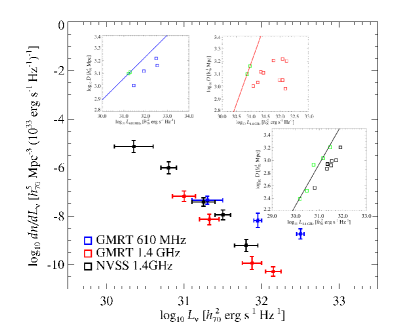
Figure 9: RH luminosity function obtained from existent observations. The insets show the sample luminosity-distance distributions (see main text for details) where the solid line is the fit to the upper envelope population (indicated in green) employed to calculate the flux limit for the classical $V_{\mathrm{max}}$ estimator. The choice of the upper envelope population is somehow arbitrary, particularly in the GMRT cases due to the poor luminosity–distance distributions. The horizontal error bars represent the mass bins while the vertical error bars are Poissonian uncertainties.

References

- Abramowitz & Stegun (1965) Abramowitz M., Stegun I. A., 1965, Handbook of mathematical functions with formulas, graphs, and mathematical tables
- Basu (2012) Basu K., 2012, MNRAS, 421, L112
- Battaglia et al. (2012) Battaglia N., Bond J. R., Pfrommer C., Sievers J. L., 2012, ApJ, 758, 74
- Blasi & Colafrancesco (1999) Blasi P., Colafrancesco S., 1999, Astroparticle Physics, 12, 169
- Blasi et al. (2007) Blasi P., Gabici S., Brunetti G., 2007, International Journal of Modern Physics A, 22, 681
- Boehringer et al. (1998) Boehringer H., Tanaka Y., Mushotzky R. F., Ikebe Y., Hattori M., 1998, A&A, 334, 789
- Bonafede et al. (2010) Bonafede A., Feretti L., Murgia M., Govoni F., Giovannini G., Dallacasa D., Dolag K., Taylor G. B., 2010, A&A, 513, A30+
- Briel et al. (1992) Briel U. G., Henry J. P., Boehringer H., 1992, A&A, 259, L31
- Broderick et al. (2012) Broderick A. E., Chang P., Pfrommer C., 2012, ApJ, 752, 22
- Brown & Rudnick (2011) Brown S., Rudnick L., 2011, MNRAS, 412, 2
- Brown et al. (2011) Brown S., Emerick A., Rudnick L., Brunetti G., 2011, ApJL, 740, L28
- Brunetti & Blasi (2005) Brunetti G., Blasi P., 2005, MNRAS, 363, 1173
- Brunetti & Lazarian (2007) Brunetti G., Lazarian A., 2007, MNRAS, 378, 245
- Brunetti & Lazarian (2011) Brunetti G., Lazarian A., 2011, MNRAS, 410, 127
- Brunetti et al. (2004) Brunetti G., Blasi P., Cassano R., Gabici S., 2004, MNRAS, 350, 1174
- Brunetti et al. (2008) Brunetti G., et al., 2008, Nature, 455, 944
- Brunetti et al. (2009) Brunetti G., Cassano R., Dolag K., Setti G., 2009, A&A, 507, 661
- Brunetti et al. (2012) Brunetti G., Blasi P., Reimer O., Rudnick L., Bonafede A., Brown S., 2012, MNRAS, 426, 956
- Cappelluti et al. (2011) Cappelluti N., et al., 2011, Memorie della Societa Astronomica Italiana Supplementi, 17, 159
- Cassano & Brunetti (2005) Cassano R., Brunetti G., 2005, MNRAS, 357, 1313
- Cassano et al. (2007) Cassano R., Brunetti G., Setti G., Govoni F., Dolag K., 2007, MNRAS, 378, 1565
- Cassano et al. (2010) Cassano R., Brunetti G., Röttgering H. J. A., Brüggen M., 2010, A&A, 509, A68
- Cassano et al. (2012) Cassano R., Brunetti G., Norris R. P., Röttgering H. J. A., Johnston-Hollitt M., Trasatti M., 2012, A&A, 548, A100
- Cassano et al. (2013) Cassano R., et al., 2013, ApJ, 777, 141
- Cavagnolo et al. (2009) Cavagnolo K. W., Donahue M., Voit G. M., Sun M., 2009, ApJs, 182, 12
- Churazov et al. (2003) Churazov E., Forman W., Jones C., Böhringer H., 2003, ApJ, 590, 225
- Croston et al. (2008) Croston J. H., et al., 2008, A&A, 487, 431
- Deiss et al. (1997) Deiss B. M., Reich W., Lesch H., Wielebinski R., 1997, A&A, 321, 55
- Dennison (1980) Dennison B., 1980, ApJl, 239, L93
- Dolag & Enßlin (2000) Dolag K., Enßlin T. A., 2000, A&A, 362, 151
- Dolag et al. (2005) Dolag K., Vazza F., Brunetti G., Tormen G., 2005, MNRAS, 364, 753
- Domainko et al. (2009) Domainko W., Nedbal D., Hinton J. A., Martineau-Huynh O., 2009, International Journal of Modern Physics D, 18, 1627
- Donnert et al. (2010a) Donnert J., Dolag K., Brunetti G., Cassano R., Bonafede A., 2010a, MNRAS, 401, 47
- Donnert et al. (2010b) Donnert J., Dolag K., Cassano R., Brunetti G., 2010b, MNRAS, 407, 1565
- Donnert et al. (2013) Donnert J., Dolag K., Brunetti G., Cassano R., 2013, MNRAS, 429, 3564
- Dubois & Teyssier (2008) Dubois Y., Teyssier R., 2008, A&A, 482, L13
- Eckert et al. (2008) Eckert D., Produit N., Paltani S., Neronov A., Courvoisier T. J.-L., 2008, A&A, 479, 27
- Enßlin & Röttgering (2002) Enßlin T. A., Röttgering H., 2002, A&A, 396, 83
- Enßlin et al. (2011) Enßlin T., Pfrommer C., Miniati F., Subramanian K., 2011, A&A, 527, A99+
- Fabian et al. (2006) Fabian A. C., Sanders J. S., Taylor G. B., Allen S. W., Crawford C. S., Johnstone R. M., Iwasawa K., 2006, MNRAS, 366, 417
- Fabian et al. (2011) Fabian A. C., et al., 2011, MNRAS, 418, 2154
- Felice & Kulsrud (2001) Felice G. M., Kulsrud R. M., 2001, ApJ, 553, 198
- Felten (1976) Felten J. E., 1976, ApJ, 207, 700
- Feretti et al. (2001) Feretti L., Fusco-Femiano R., Giovannini G., Govoni F., 2001, A&A, 373, 106
- Feretti et al. (2012) Feretti L., Giovannini G., Govoni F., Murgia M., 2012, A&Ar, 20, 54
- Fermi-LAT Collaboration (2009) Fermi-LAT Collaboration 2009, ApJ, 699, 31
- Fermi-LAT Collaboration (2010a) Fermi-LAT Collaboration 2010a, JCAP, 5, 25
- Fermi-LAT Collaboration (2010b) Fermi-LAT Collaboration 2010b, ApJl, 717, L71
- Fermi-LAT Collaboration (2014) Fermi-LAT Collaboration 2014, ApJ, 787, 18
- Fujita et al. (2008) Fujita Y., et al., 2008, PASJ, 60, 1133
- Galante et al. (2009) Galante N., et al., 2009, ArXiv:0907.5000,
- Giacintucci et al. (2014) Giacintucci S., Markevitch M., Venturi T., Clarke T. E., Cassano R., Mazzotta P., 2014, ApJ, 781, 9
- Giovannini et al. (1993) Giovannini G., Feretti L., Venturi T., Kim K. T., Kronberg P. P., 1993, ApJ, 406, 399
- Giovannini et al. (1999) Giovannini G., Tordi M., Feretti L., 1999, New A, 4, 141
- Gitti et al. (2002) Gitti M., Brunetti G., Setti G., 2002, A&A, 386, 456
- Govoni et al. (2009) Govoni F., Murgia M., Markevitch M., Feretti L., Giovannini G., Taylor G. B., Carretti E., 2009, A&A, 499, 371
- HESS Collaboration (2009a) HESS Collaboration 2009a, A&A, 495, 27
- HESS Collaboration (2009b) HESS Collaboration 2009b, A&A, 502, 437
- HESS Collaboration (2012) HESS Collaboration 2012, A&A, 545, A103
- Han et al. (2012) Han J., Frenk C. S., Eke V. R., Gao L., White S. D. M., Boyarsky A., Malyshev D., Ruchayskiy O., 2012, MNRAS, 427, 1651
- Huber et al. (2013) Huber B., Tchernin C., Eckert D., Farnier C., Manalaysay A., Straumann U., Walter R., 2013, A&A, 560, A64
- Kale et al. (2013) Kale R., Venturi T., Giacintucci S., Dallacasa D., Cassano R., Brunetti G., Macario G., Athreya R., 2013, A&A, 557, A99
- Kang & Ryu (2011) Kang H., Ryu D., 2011, ApJ, 734, 18
- Kang et al. (2012) Kang H., Ryu D., Jones T. W., 2012, ApJ, 756, 97
- Keshet (2010) Keshet U., 2010, ArXiv:1011.0729,
- Keshet & Loeb (2010) Keshet U., Loeb A., 2010, ApJ, 722, 737
- Kiuchi et al. (2009) Kiuchi R., et al., 2009, ApJ, 704, 240
- Kuchar & Enßlin (2011) Kuchar P., Enßlin T. A., 2011, A&A, 529, A13+
- Kulsrud & Pearce (1969) Kulsrud R., Pearce W. P., 1969, ApJ, 156, 445
- Kushnir et al. (2009) Kushnir D., Katz B., Waxman E., 2009, JCAP, 9, 24
- Lau et al. (2009) Lau E. T., Kravtsov A. V., Nagai D., 2009, ApJ, 705, 1129
- MAGIC Collaboration (2010) MAGIC Collaboration 2010, ApJ, 710, 634
- MAGIC Collaboration (2012) MAGIC Collaboration 2012, A&A, 541, A99
- Million et al. (2010) Million E. T., Allen S. W., Werner N., Taylor G. B., 2010, MNRAS, 405, 1624
- Miniati (2003) Miniati F., 2003, MNRAS, 342, 1009
- Miniati et al. (2001a) Miniati F., Ryu D., Kang H., Jones T. W., 2001a, ApJ, 559, 59
- Miniati et al. (2001b) Miniati F., Jones T. W., Kang H., Ryu D., 2001b, ApJ, 562, 233
- Murgia et al. (2009) Murgia M., Govoni F., Markevitch M., Feretti L., Giovannini G., Taylor G. B., Carretti E., 2009, A&A, 499, 679
- Murgia et al. (2010) Murgia M., Eckert D., Govoni F., Ferrari C., Pandey-Pommier M., Nevalainen J., Paltani S., 2010, A&A, 514, A76
- Nevalainen et al. (2009) Nevalainen J., Eckert D., Kaastra J., Bonamente M., Kettula K., 2009, A&A, 508, 1161
- Norris et al. (2011) Norris R. P., et al., 2011, PASA, 28, 215
- Pedlar et al. (1990) Pedlar A., Ghataure H. S., Davies R. D., Harrison B. A., Perley R., Crane P. C., Unger S. W., 1990, MNRAS, 246, 477
- Pérez-Torres et al. (2009) Pérez-Torres M. A., Zandanel F., Guerrero M. A., Pal S., Profumo S., Prada F., Panessa F., 2009, MNRAS, 396, 2237
- Perkins (2008) Perkins J. S., 2008, in Aharonian F. A., Hofmann W., Rieger F., eds, American Institute of Physics Conference Series Vol. 1085, American Institute of Physics Conference Series. pp 569–572, doi:10.1063/1.3076736
- Perkins et al. (2006) Perkins J. S., et al., 2006, ApJ, 644, 148
- Pfrommer (2008) Pfrommer C., 2008, MNRAS, 385, 1242
- Pfrommer & Enßlin (2003) Pfrommer C., Enßlin T. A., 2003, A&A, 407, L73
- Pfrommer & Enßlin (2004a) Pfrommer C., Enßlin T. A., 2004a, MNRAS, 352, 76
- Pfrommer & Enßlin (2004b) Pfrommer C., Enßlin T. A., 2004b, A&A, 413, 17
- Pfrommer et al. (2006) Pfrommer C., Springel V., Enßlin T. A., Jubelgas M., 2006, MNRAS, 367, 113
- Pfrommer et al. (2007) Pfrommer C., Enßlin T. A., Springel V., Jubelgas M., Dolag K., 2007, MNRAS, 378, 385
- Pfrommer et al. (2008) Pfrommer C., Enßlin T. A., Springel V., 2008, MNRAS, 385, 1211
- Pinzke & Pfrommer (2010) Pinzke A., Pfrommer C., 2010, MNRAS, 409, 449
- Pinzke et al. (2011) Pinzke A., Pfrommer C., Bergström L., 2011, Phys. Rev. D,, 84, 123509
- Pinzke et al. (2013) Pinzke A., Oh S. P., Pfrommer C., 2013, MNRAS,
- Planck Collaboration (2014) Planck Collaboration 2014, A&A, 571, A20
- Prokhorov & Churazov (2014) Prokhorov D. A., Churazov E. M., 2014, A&A, 567, A93
- Reimer et al. (2003) Reimer O., Pohl M., Sreekumar P., Mattox J. R., 2003, ApJ, 588, 155
- Reiprich & Böhringer (2002) Reiprich T. H., Böhringer H., 2002, ApJ, 567, 716
- Riebe et al. (2013) Riebe K., et al., 2013, Astronomische Nachrichten, 334, 691
- Röttgering et al. (2012) Röttgering H., et al., 2012, Journal of Astrophysics and Astronomy, p. 34
- Rudnick (2002) Rudnick L., 2002, PASP, 114, 427
- Ryu et al. (2003) Ryu D., Kang H., Hallman E., Jones T. W., 2003, ApJ, 593, 599
- Ryu et al. (2008) Ryu D., Kang H., Cho J., Das S., 2008, Science, 320, 909
- Schlickeiser (2002) Schlickeiser R., 2002, Cosmic ray astrophysics. Springer. ISBN 3-540-66465-3, http://esoads.eso.org/cgi-bin/nph-bib_query?bibcode=2002cra..book.....S&db_key=AST
- Schlickeiser et al. (1987) Schlickeiser R., Sievers A., Thiemann H., 1987, A&A, 182, 21
- Schuecker et al. (2004) Schuecker P., Finoguenov A., Miniati F., Böhringer H., Briel U. G., 2004, A&A, 426, 387
- Sijbring (1993) Sijbring L. G., 1993, PhD thesis, Groningen University
- Skillman et al. (2008) Skillman S. W., O’Shea B. W., Hallman E. J., Burns J. O., Norman M. L., 2008, ApJ, 689, 1063
- Skillman et al. (2013) Skillman S. W., Xu H., Hallman E. J., O’Shea B. W., Burns J. O., Li H., Collins D. C., Norman M. L., 2013, ApJ, 765, 21
- Sommer & Basu (2014) Sommer M. W., Basu K., 2014, MNRAS, 437, 2163
- Subramanian et al. (2006) Subramanian K., Shukurov A., Haugen N. E. L., 2006, MNRAS, 366, 1437
- Sutter & Ricker (2012) Sutter P. M., Ricker P. M., 2012, ApJ, 759, 92
- VERITAS Collaboration (2009) VERITAS Collaboration 2009, ApJl, 706, L275
- VERITAS Collaboration (2012) VERITAS Collaboration 2012, ApJ, 757, 123
- Vazza et al. (2009) Vazza F., Brunetti G., Gheller C., 2009, MNRAS, 395, 1333
- Venturi et al. (2007) Venturi T., Giacintucci S., Brunetti G., Cassano R., Bardelli S., Dallacasa D., Setti G., 2007, A&A, 463, 937
- Venturi et al. (2008) Venturi T., Giacintucci S., Dallacasa D., Cassano R., Brunetti G., Bardelli S., Setti G., 2008, A&A, 484, 327
- Vestrand (1982) Vestrand W. T., 1982, AJ, 87, 1266
- Vikhlinin et al. (2005) Vikhlinin A., Markevitch M., Murray S. S., Jones C., Forman W., Van Speybroeck L., 2005, ApJ, 628, 655
- Völk et al. (1996) Völk H. J., Aharonian F. A., Breitschwerdt D., 1996, Space Science Reviews, 75, 279
- Watanabe et al. (2001) Watanabe M., Yamashita K., Furuzawa A., Kunieda H., Tawara Y., 2001, PASJ, 53, 605
- Wiener et al. (2013) Wiener J., Oh S. P., Guo F., 2013, MNRAS, 434, 2209
- Zandanel et al. (2014) Zandanel F., Pfrommer C., Prada F., 2014, MNRAS, 438, 116
- van Weeren et al. (2012) van Weeren R. J., et al., 2012, A&A, 543, A43