A Phenomenological Model for the Intracluster Medium that matches X-ray and Sunyaev-Zel’dovich observations

Abstract

Cosmological hydrodynamical simulations of galaxy clusters are still challenged to produce a model for the intracluster medium that matches all aspects of current X-ray and Sunyaev-Zel’dovich observations. To facilitate such comparisons with future simulations and to enable realistic cluster population studies for modeling e.g., non-thermal emission processes, we construct a phenomenological model for the intracluster medium that is based on a representative sample of observed X-ray clusters. We create a mock galaxy cluster catalog based on the large collisionless $N$-body simulation MultiDark, by assigning our gas density model to each dark matter cluster halo. Our clusters are classified as cool-core and non cool-core according to a dynamical disturbance parameter. We demonstrate that our gas model matches the various observed Sunyaev-Zel’dovich and X-ray scaling relations as well as the X-ray luminosity function, thus enabling to build a reliable mock catalog for present surveys and forecasts for future experiments. In a companion paper, we apply our catalogs to calculate non-thermal radio and gamma-ray emission of galaxy clusters. We make our cosmologically complete multi-frequency mock catalogs for the (non-)thermal cluster emission at different redshifts publicly and freely available online through the MultiDark database.

1 Introduction

Galaxy clusters are the rarest and largest gravitationally-collapsed objects in the Universe and form at sites of constructive interference of long waves in the primordial density fluctuations. Clusters reach radial extends of a few Mpc and total masses $M\sim(10^{14}-10^{15})M_{\odot}$, of which galaxies, hot ($1-10$ keV) gas and dark matter (DM) contribute roughly 5, 15 and 80 per cent, respectively. If the thermal properties of the intracluster medium (ICM) were solely determined by the gravity of the system, then clusters would obey self-similar scaling relations (Kaiser, 1986). However, X-ray observations have demonstrated that self-similarity is broken, especially at low-mass scales (see, e.g., Voit, 2005 for a review). Apparently the energy input from non-gravitational processes associated with galaxy formation have a larger influence in smaller systems, i.e., at scales of galaxy groups.

The central cooling time of the X-ray emitting gas in galaxy clusters and groups is bimodally distributed. Approximately half of all systems have radiative cooling times of less than 1 Gyr and establish a population of cool core clusters (CCCs), while others have cooling times that can be longer than the age of the Universe, forming the non-cool core cluster (NCCC) population (Cavagnolo et al., 2009; Hudson et al., 2010). Several physical processes have been proposed to be responsible for balancing radiative cooling of the low-entropy gas at the centers of CCCs. In particular feedback by active galactic nuclei (AGN) has come into the focus of recent research (McNamara & Nulsen, 2007, 2012), owing to the self-regulated nature of the proposed feedback and observational correlations between radio activity and central entropy (which is a proxy for a small cooling time). The underlying physical processes responsible for the heating include dissipation of mechanical heating by outflows, lobes, or sound waves from the central AGN (e.g., Churazov et al., 2001; Brüggen & Kaiser, 2002; Ruszkowski & Begelman, 2002; Gaspari et al., 2012) or cosmic-ray heating: streaming cosmic rays excite Alfvén waves on which they resonantly scatter (Kulsrud & Pearce, 1969). Damping of these waves transfers cosmic ray energy and momentum to the cooling plasma (Loewenstein et al., 1991; Guo & Oh, 2008; Enßlin et al., 2011; Wiener et al., 2013), heating it at a rate that balances radiative cooling on average at each radius while explaining the observed temperature floor in CCCs by thermal stability of the heating mechanism (Pfrommer, 2013).

Modeling the formation and evolution of clusters with cosmological hydrodynamical simulations has been progressively refined over the last years to also include (sub-resolution models for) AGN feedback (e.g., Sijacki et al., 2007, 2008; Puchwein et al., 2008; Dubois et al., 2012; Gaspari et al., 2012; Vazza et al., 2013). While the comparison between data and simulations with AGN feedback improved for integrated thermal properties of large cluster samples (Battaglia et al., 2012a, b), there are still notable differences for differential quantities such as the pressure profile (Planck Collaboration et al., 2013) or the profile of gas mass fractions (Battaglia et al., 2013). These discrepancies (that have been more dramatic in the past without AGN feedback) motivated the development of phenomenological models of the ICM (e.g., Ostriker et al., 2005; Capelo et al., 2012). Here, we construct a simple and purely phenomenological model that matches all available X-ray and Sunyaev-Zel’dovich (SZ) data with the goal to facilitate comparison with future hydrodynamical simulations, to allow the modeling of non-thermal cluster emission over the entire electromagnetic wave-band, and finally to enable the construction of cluster mock catalogs of the thermal and non-thermal cluster emission (in the radio, hard X-ray, and gamma-ray band) of current and future surveys. Such a model for the ICM needs to be applied to a sample of cluster halos, which can either be obtained by means of analytical expressions for the cluster mass function (e.g., Jenkins et al., 2001) or cosmological simulations. In this work, we make use of the recent large-volume $N$-body simulation MultiDark, which employs a flat $\Lambda$ Cold Dark Matter cosmology (Prada et al., 2012).

Our phenomenological approach uses gas density profiles of a representative sample of observed X-ray clusters, which are complemented by the observed cluster mass-dependent gas mass fractions. The resulting cluster mock sample are then compared to data including the X-ray luminosity function (XLF), the luminosity-mass relation, $L_{\mathrm{X}}-M$, and the $Y_{\mathrm{X}}-M$ relation, where $Y_{\mathrm{X}}=M_{\mathrm{gas}}k_{\mathrm{B}}T$ with an X-ray-derived gas mass $M_{\mathrm{gas}}$ and temperature $T$ (Kravtsov et al., 2006). We additionally compare our $Y_{\mathrm{SZ}}-M$ relation to recent SZ data, where $Y_{\mathrm{SZ}}$ denotes the integrated Compton-$y$ parameter. In a companion paper (Zandanel et al., 2014; hereafter Paper II), we apply our ICM model to predict the non-thermal radio and gamma-ray emission of a cosmological complete sample of galaxy clusters, enabling valuable insight into the statistics of radio halos. One of our final data products is a complete cosmological cluster mock catalog, at different redshifts, containing information of the DM and ICM properties for each object, together with its (non-)thermal emission at different frequencies. All the products can be found on-line at the MultiDark database (www.multidark.org).

In Section 2, we introduce the MultiDark simulation along with our selected cluster halo sample. We assign to each of our clusters the phenomenologically constructed gas density profile in Section 3. In Sections 4 and 5, we show that this approach can successfully reproduce the observed X-ray and SZ cluster data. We present the resulting mock cluster catalogs in Section 6, and eventually summarize in Section 7. In this work, the cluster mass $M_{\Delta}$ and radius $R_{\Delta}$ are defined with respect to a density that is $\Delta=200$ or 500 times the critical density of the Universe. We adopt density parameters of $\Omega_{\mathrm{m}}=0.27$, $\Omega_{\Lambda}=0.73$ and today’s Hubble constant of $H_{0}=100\,h_{70}$ km s^-1 Mpc^-1 where $h_{70}=0.7$.

2 MultiDark simulation and final cluster sample

The MultiDark simulation used in this work is described in detail in Prada et al. (2012). It is an $N$-body cosmological simulation done with the Adaptive-Refinement-Tree (ART) code (Kravtsov et al., 1997) of $2048^{3}$ particles within a ($1000\,h^{-1}$ Mpc)³ cube. The adopted cosmological parameters are $\Omega_{\mathrm{m}}=0.27$, $\Omega_{\Lambda}=0.73$, $\Omega_{\mathrm{b}}=0.0469$, $n_{\mathrm{s}}=0.95$, $h=0.7$ and $\sigma_{8}=0.82$. This simulation is particularly well suited for our purpose because of its large number of high-mass objects, i.e., galaxy clusters.

We use the MultiDark halo catalog from its on-line database, constructed with the Bound Density Maxima (BDM) algorithm (Klypin & Holtzman, 1997). We will mainly use $M_{500}$ and $R_{500}$ for comparison with existing observational works. We use the technique described in Hu & Kravtsov (2003) to convert $M_{200}$ and $R_{200}$ provided by the MultiDark halo catalog to $M_{500}$ and $R_{500}$. In creating our cluster sample we only select distinct halos, i.e., those halos that are not sub-halos of any other halo, which by definition are not galaxy clusters.

Additionally, we assume that the main emission mechanism in the ICM is thermal bremsstrahlung, which is true only above a particle energy of approximately $2.6$ keV (Sarazin, 1988). Below this energy, there could be other important contributions to the emission, e.g., from atomic lines. Therefore, we impose a mass cut of $M_{200}\geq 1\times 10^{14}$ $h^{-1}$ M${}_{\odot}\approx 1.4\times 10^{14}$ $h_{70}^{-1}$ M_⊙ which ensures $k_{\mathrm{B}}T\gtrsim 2.6$ keV (assuming the $M_{500}-T_{\mathrm{ci}}$ relation of Mantz et al. 2010b).

In Paper II, we present predictions for the LOFAR radio observatory which expects to detect diffuse radio emission in clusters up to redshift $z\approx 1$ (e.g., Röttgering et al., 2012). Thus, we make use of different simulation snapshots up to $z=1$. The extrapolation of our model beyond this redshift is rather uncertain as it is based on observations at low(er) redshift. In Table 1, we show the total cluster number in our final cluster sample at different redshifts.

Table 1: Number of halos in the final cluster sample

| redshift $z$	number of halos
0.0	13763
0.1	12398
0.18	11106
0.2	10783
0.4	7789
0.53	6079
0.61	5187
0.78	3372
1.0	1803

Note. We show the number of halos in our MultiDark snapshots at redshift $z$ for $M_{200}\geq 1\times 10^{14}$ $h^{-1}$ M${}_{\odot}\approx 1.4\times 10^{14}$ $h_{70}^{-1}$ M_⊙. More snapshots can be found online at www.mutlidark.org.

3 Gas density modeling

We decided to use a phenomenological approach and construct the gas density profiles directly from X-ray observations. A suitable X-ray sample that provides the required information is the Representative XMM-Newton Cluster Structure Survey (REXCESS) sample (Croston et al., 2008; Pratt et al., 2009). It is a sample of 31 galaxy clusters of different dynamical states at redshifts $0.06<z<0.18$ with detailed information on the de-projected electron density profiles (Croston et al., 2008). In Fig. 1, we show the 31 electron density profiles of the REXCESS sample color-coded by NCCCs and CCCs.

In order to obtain an electron density profile that we will attach to our simulated clusters, we use a generalized Navarro-Frank-White (GNFW) profile,

$$n_{\mathrm{e}}(x)=\frac{n_{0}}{x^{\beta}\left[1+x^{\alpha}\right]^{\frac{\delta-\beta}{\alpha}}},$$ (1)

where $x=R/R_{\mathrm{c}}$ and $R_{\mathrm{c}}$ is the cluster core radius. To reduce the dimensionality of our fit, we fix representative values of $R_{\mathrm{c}}=0.2\,R_{500}$, $\alpha=1$ and $\delta=2.5$. We fit the radial density profiles of the REXCESS sample in log-log space, separating them in the two categories of NCCCs and CCCs as shown in Fig. 1. We obtain $n_{\mathrm{0,NCCC}}=1.02\times 10^{-2}$ $h_{70}^{1/2}$ cm^-3, $n_{\mathrm{0,CCC}}=8.32\times 10^{-3}$ $h_{70}^{1/2}$ cm^-3, $\beta_{\mathrm{NCCC}}=-0.093$, and $\beta_{\mathrm{CCC}}=0.592$. The resulting fits are shown in blue and red for the NCCC and CCC population, respectively.

The next step is to introduce a mass-scaling in order to apply our GNFW profiles to clusters of all masses. We adopt the gas mass fraction-mass scaling, $f_{\mathrm{gas},500}-M_{500}$ of Sun et al. (2009) (and adopt their equation (8)). We can express $f_{\mathrm{gas},500}$ in the following way:

$$f_{\mathrm{gas},500}=\frac{M_{\mathrm{gas},500}}{M_{500}}=\frac{\int_{0}^{R_{500}}\rho_{\mathrm{gas}}\mathrm{d}V}{M_{500}}$$ (2)

with $\rho_{\mathrm{gas}}(R)=\rho_{\mathrm{gas}}=n_{\mathrm{e}}m_{\mathrm{p}}/(X_{\mathrm{H}}X_{\mathrm{e}})$ where $m_{\mathrm{p}}$ is the proton mass, $X_{\mathrm{H}}=0.76$ is the primordial hydrogen mass fraction and $X_{\mathrm{e}}=1.157$ the ratio of electron-to-hydrogen number densities in the fully ionized ICM (Sarazin, 1988). For each cluster $i$ of our sample, we then define a mass-scaled gas profile as $\rho_{\mathrm{gas},i}=C_{i}\,\rho_{\mathrm{gas}}$ with:

$$C_{i} = (0.0656\pm(0.0064g_{1}))\,h_{70}^{-1.5}$$

$$\times \left(\frac{M_{500,i}}{1.04\times 10^{13}h_{70}^{-1}\mathrm{M_{\odot}}}\right)^{0.135\pm(0.030g_{2})}\frac{M_{500,i}}{\int_{0}^{R_{500,i}}\rho_{\mathrm{gas}}\mathrm{d}V}$$

where $g_{1}$ and $g_{2}$ are random Gaussian numbers, which we use in order to simulate the natural scatter of the gas profiles.

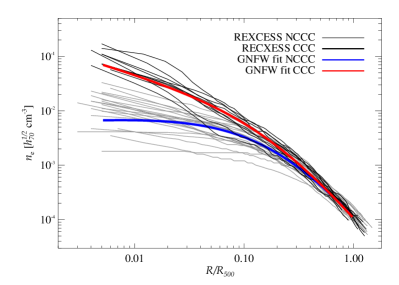
Figure 1: Electron density profiles of the 31 clusters in the REXCESS sample. Grey and black lines represent NCCCs and CCCs, respectively. The blue and red lines represent our GNFW mean profile for the NCCCs and CCCs, respectively.

Hence, for each cluster in our sample we obtain a gas density profile $\rho_{\mathrm{gas},i}$ that obeys the observed $f_{\mathrm{gas},500}-M_{500}$ relation and is uniquely determined by its total mass $M_{500,i}$ and by the property of being a NCCC or CCC. We assign the latter property to every halo depending on its merging history. In particular, we make use of the offset parameter $X_{\mathrm{off}}$ computed for the MultiDark halo catalog. This is defined as the distance from the halo center to the center of mass in units of the virial radius. This parameter assesses the dynamical state of the cluster and whether the halo has experienced a recent merger or not. Current observations reveal a ratio of NCCCs and CCCs of about 50 per cent (e.g., Chen et al., 2007; Sanderson et al., 2009). Since there is a correlation between merging clusters and NCCCs, we use the median of the $X_{\mathrm{off}}$ distribution to separate our sample into CCCs and NCCCs (with NCCCs defined to be those halos with the larger dynamical offsets). Clearly, this is an over-simplification, and future X-ray surveys will have to determine this property also as a function of redshift.

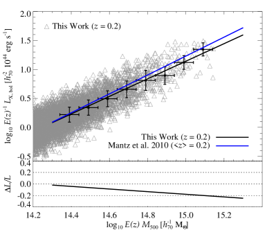
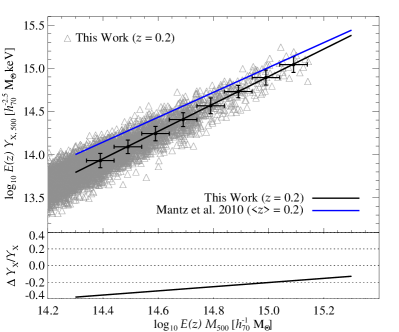
Figure 2: X-ray cluster scaling relations. Grey triangles show the MultiDark sample (limited to the mass range covered by observations), the black line is the corresponding scaling relation, and the blue line is the observational result by Mantz et al. (2010b). The black crosses represent the median values of the quantity in question for a given mass bin (indicated by horizontal error bars), and the vertical error bars represent the standard deviation within a bin. The bottom panels show the relative difference to the observational scaling relations. Left. We compare the bolometric X-ray luminosity-to-mass relation, $L_{\mathrm{bol}}-M_{500}$, at $z=0.2$ to the observational sample by Mantz et al. (2010b) with a median of $z\approx 0.2$. Right. $Y_{\mathrm{X}}-M_{500}$ scaling relation of our model in comparison to the observational sample by Mantz et al. (2010b).

We also account for redshift evolution of the gas profiles. While our NCCC and CCC gas profiles as derived from the REXCESS cluster sample are merely used to define a profile shape, the normalization of the gas profiles is set by the observational $f_{\mathrm{gas},500}-M_{500}$ relation (Sun et al., 2009). The 43 clusters used in Sun et al. (2009) have redshifts $0.012<z<0.12$ with a median of $z\approx 0.04$. Thus, our phenomenological gas profile is representative of the cluster population at $z\approx 0$. To extend this profile to high-$z$, we adopt a self-similar scaling of the gas density as $\rho_{\mathrm{gas}}(z)=E(z)^{2}\rho_{\mathrm{gas}}(z=0)$, where $E(z)^{2}=\Omega_{\mathrm{m}}(1+z)^{3}+\Omega_{{\Lambda}}$.

As a cautionary remark, we emphasize that our model has been constructed to be valid within $R_{500}$ and more work is needed to extrapolate it to larger cluster radii, particularly for the thermal cluster emission. Those cluster regions are characterized by a steadily increasing level of kinetic-to-thermal pressure support (e.g., Lau et al., 2009; Battaglia et al., 2012a), density clumping (Nagai & Lau, 2011; Battaglia et al., 2013), and asphericity and ellipticity of the halo morphologies (Battaglia et al., 2013), in particular beyond the virial radius where the filamentary cosmic web connects to the cluster interiors.

4 X-ray observables

So far, we used a well-observed representative sample of X-ray clusters (REXCESS) that was supplemented with X-ray data on gas mass fractions to construct our phenomenological gas model. Here, we will test how our cluster mock data compare to various X-ray inferred observables, which are obtained from different cluster samples and from (partially) different X-ray observatories. Those include the observed $L_{\mathrm{bol}}-M_{500}$ relation, the $Y_{X}-M_{500}$ relation, and the XLF.

4.1 Scaling Relations

First, we calculate the bolometric thermal bremsstrahlung luminosity $L_{\mathrm{bol}}$ following Sarazin (1988). To assign a temperature to our model clusters (that is needed for calculating $L_{\mathrm{bol}}$ and $Y_{\mathrm{X}}$), we adopt the $T-M_{500}$ relation by Mantz et al. (2010b),

$$\log_{10}\left(\frac{k_{\mathrm{B}}T_{\mathrm{ci}}}{\mathrm{keV}}\right)=A+B~{}\log_{10}\left(\frac{E(z)M_{500}}{10^{15}h_{70}^{-1}\mathrm{M_{\odot}}}\right)$$ (4)

where $A=0.91$, $B=0.46$, and $T_{\mathrm{ci}}$ is the cluster temperature not centrally excised (Mantz et al., 2010b). Mantz et al. (2010b) report a scatter of $\sigma_{\mathrm{yx}}=0.06,$ which we apply to our sample using Gaussian deviates.

In the left panel of Fig. 2, we show how our model $L_{\mathrm{bol}}-M_{500}$ relation compares with observations by Mantz et al. (2010b) (all data, see their Table 7). Their sample is composed of 238 clusters at $0.02<z<0.46$ with a median of $z\approx 0.2$ and self-consistently takes into account all selection effects, covariances, systematic uncertainties and the cluster mass function (Mantz et al., 2010a). For this reason, we compare the Mantz et al. (2010b) data to our model at $z=0.2$, and limit the comparison to the mass range covered by the observations. Overall, there is reassuring agreement between our phenomenological model and the data, which probe our model most closely on scales around the cluster core radii (which is where the contribution to $L_{\mathrm{X}}$ per logarithmic interval in radius, $\mathrm{d}L_{\mathrm{X}}/\mathrm{d}\log r\propto r^{3}n_{\rm{gas}}^{2}(r)\sqrt{k_{\mathrm{B}}T}$, approximately attains its maximum). In Table 2, we show our model $L_{\mathrm{bol}}-M_{500}$ scaling relation and its scatter for different redshifts. We find that the scatter of our samples at all redshifts are Gaussian distributed with a standard deviation of $\sigma_{yx}\approx 0.18$ that matches the observational results of Mantz et al. (2010b), which report a scatter of $\sigma_{yx}=0.185$.

In the right panel of Fig. 2, we compare the $Y_{\mathrm{X}}-M_{500}$ relation of our sample to observational data (Mantz et al., 2010b). The model agrees nicely at the high-mass end, but underpredicts the observed scaling at low masses. The differential contribution to the thermal energy per logarithmic interval in radius (and hence to the integrated Compton-$y$ parameter) is given by $\mathrm{d}Y/\mathrm{d}\log r\propto r^{3}P_{\mathrm{th}}(r)$, with the thermal gas pressure $P_{\mathrm{th}}=n_{\mathrm{gas}}k_{\mathrm{B}}T$. It peaks at scales slightly smaller than $R_{500}$ with 1-$\sigma$ contributions extending out to $3\,R_{500}$ (Battaglia et al., 2010). Hence, the observational scaling constrains our model on those large scales, quite complementary to the X-ray luminosity. The deviations at small masses either indicate tensions with our assumptions on $f_{\mathrm{gas}}$, the gas temperature, or different selection effects of either observational sample that we use for model calibration and comparison. Mantz et al. (2010b) determine their masses by adopting a constant value for $f_{\mathrm{gas}}$, in contrast to our approach which adopts the observed $f_{\mathrm{gas},500}-M_{500}$ relation given by Sun et al. (2009). Additionally, we adopt the Mantz et al. (2010b) centrally included temperature throughout all our work, while Mantz et al. (2010b) use the centrally excised temperature to calculate $Y_{\mathrm{X}}$. This assumption also impacts the scatter of the $Y_{\mathrm{X}}-M$ relation. In fact, using the centrally included temperature, we found a scatter of $\sigma_{yx}\approx 0.11$ (see Table 3 where our $Y_{\mathrm{X}}$ scaling relations are reported), significantly higher than the value of $\sigma_{yx}=0.052$ found by Mantz et al. (2010b).

Table 2: $L_{\mathrm{bol}}-M_{500}$ scaling relations.

| redshift $z$	$A$	$B$	$\sigma_{yx}$
0	$-21.41\pm 0.11$	$1.50\pm 0.01$	0.179
0.1	$-21.33\pm 0.12$	$1.50\pm 0.01$	0.179
0.18	$-21.56\pm 0.13$	$1.51\pm 0.01$	0.177
0.2	$-21.58\pm 0.13$	$1.51\pm 0.01$	0.178
0.4	$-21.30\pm 0.17$	$1.49\pm 0.01$	0.178
0.53	$-21.68\pm 0.20$	$1.52\pm 0.01$	0.175
0.61	$-21.87\pm 0.22$	$1.53\pm 0.01$	0.177
0.78	$-21.08\pm 0.29$	$1.48\pm 0.02$	0.177
1	$-20.91\pm 0.42$	$1.46\pm 0.03$	0.177

Note. Scaling relations are reported in the form of $\log_{10}~{}(L_{\mathrm{bol}}~{}/~{}E(z)~{}h_{70}^{-2}~{}10^{44}~{}\mathrm{erg~{}s}^{-1})=A+B~{}\log_{10}~{}(E(z)~{}M_{500}~{}/~{}h_{70}^{-1}~{}\mathrm{M_{\odot}})$. The relation scatter $\sigma_{yx}$ is also shown.

Table 3: $Y_{\mathrm{X},500}-M_{500}$ scaling relations.

| redshift $z$	$A$	$B$	$\sigma_{yx}$
0	$-9.09\pm 0.07$	$1.60\pm 0.01$	0.109
0.1	$-8.94\pm 0.07$	$1.59\pm 0.01$	0.109
0.18	$-8.97\pm 0.08$	$1.59\pm 0.01$	0.109
0.2	$-8.91\pm 0.08$	$1.59\pm 0.01$	0.109
0.4	$-8.94\pm 0.10$	$1.59\pm 0.01$	0.108
0.53	$-9.05\pm 0.12$	$1.60\pm 0.01$	0.108
0.61	$-9.01\pm 0.14$	$1.59\pm 0.01$	0.109
0.78	$-8.76\pm 0.18$	$1.58\pm 0.01$	0.109
1	$-8.76\pm 0.26$	$1.58\pm 0.02$	0.109

Note. Scaling relations are reported in the form of $\log_{10}~{}(E(z)~{}Y_{\mathrm{X},500}~{}/~{}h_{70}^{-2.5}~{}\mathrm{M_{\odot}}~{}\mathrm{keV})=A+B~{}\log_{10}~{}(E(z)~{}M_{500}~{}/~{}h_{70}^{-1}~{}\mathrm{M_{\odot}})$. The relation scatter $\sigma_{yx}$ is also shown.

4.2 Luminosity Functions

Studies of the XLF got out of fashion during the last years due to the difficulties of using the X-ray luminosity for cosmological purposes. The X-ray emissivity scales with the square of the gas density, which makes it subject to density variations and clumping. This implies large scatter that causes a large Malmquist bias and underlines the necessity of careful mock surveys that need to address all systematics.

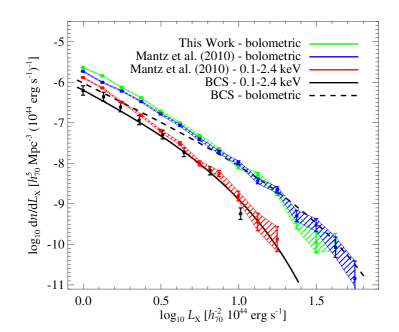
Figure 3: Bolometric and soft-band ($0.1-2.4$ keV) XLFs. Shown are the soft-band data points, the soft-band and bolometric Schechter fits of the BCS sample of Ebeling et al. (1997), which has a median of $z\approx 0.08$. While the soft-band XLF, which was obtained applying the Mantz et al. (2010b) $L_{\mathrm{X}}-M_{500}$ relation to the MultiDark $z=0.1$ snapshot, compares well with the BCS data points, it deviates from the corresponding Schechter fit. We also show the bolometric XLF of Mantz et al. (2010b) and the bolometric XLF of our model at $z=0.1$. The XLFs are calculated in equally log-spaced mass bins; the error bars represent the Poissonian errors. Note that we limit the comparison to the luminosity range covered by our sample. We impose a low-luminosity cut to avoid a drop in the XLF due to the imposed mass cut.

Nevertheless, it provides a complementary check for our model. To this end, we use the XLF of the ROSAT brightest cluster sample (BCS Ebeling et al., 1997), which is in good agreement with results from the ROSAT ESO Flux-Limited X-ray (REFLEX; Böhringer et al., 2002) and HIFLUGCS (Reiprich & Böhringer, 2002). Note that the XLF is fully determined by the mass function and the $L_{\mathrm{X}}-M_{500}$ relation after taking into account the observational biases. This means that applying the Malmquist and Eddington-bias-corrected $L_{\mathrm{X}}-M_{500}$ relation by Mantz et al. (2010b) directly to the MultiDark mass function and accounting for the observational scatter in $L_{\mathrm{X}}-M_{500}$ should yield an unbiased XLF.

We show the resulting bolometric and soft-band ($0.1-2.4$ keV) XLF in Fig. 3 and compare those to the corresponding BCS XLFs and to our model predictions. Note that there is only the Schechter fit available for the BCS bolometric XLF. While the soft-band XLF by Mantz et al. (2010b) agrees well with the BCS data points, it deviates from the corresponding Schechter fit at low luminosities. This is also true in the bolometric band, where the XLFs of Mantz et al. (2010b) and our model agree well, but deviate from the BCS Schechter fit at low luminosities. This may be an artifact due to the use of Schechter fit instead of the data points or may point to incompleteness of the BCS sample. Note that the Poissonian errors of the XLF obtained from the MultiDark simulation are a lower limit as we are neglecting the uncertainty due to cosmic variance. Studies of the XLF will become again an important topic with the upcoming launch of the eROSITA satellite (e.g., Cappelluti et al., 2011) and further studies in this direction are desirable. For these reasons, we do not show XLF predictions at other redshifts, leaving this for a future study.

5 SZ scaling relations

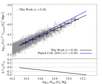
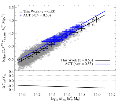
Figure 4: Comparison of our MultiDark SZ scaling relations (grey triangles) with data. The black crosses represent the $Y_{\mathrm{SZ}}$ median values of our sample for a given mass bin (indicated by horizontal error bars), and the vertical error bars represent the standard deviation within a bin. The bottom panels show the relative difference to the observational scaling relations. Left. We compare our $Y_{\mathrm{SZ}}-M$ relation at $z=0.18$ with the Planck data (blue, Planck Collaboration, 2014), which have a median redshift of about $0.18$. Right. We compare our $Y_{\mathrm{SZ}}-M$ relation at $z=0.53$ with the ACT sample (blue, Hasselfield et al., 2013) assuming a self-similar redshift evolution.

In the left panel of Fig. 4, we compare the $Y_{\mathrm{SZ}}-M_{500}$ relation of our model (following Battaglia et al., 2012a, equation 3) with the observed scaling relation by the Planck Collaboration (2014). We use the Planck COSMO sample, which is Malmquist-bias corrected and has a median redshift of $0.18$, and compare this to our $z=0.18$ relation. Our model reproduces the normalization of the scaling relation remarkably well, except for the high-mass end where our simulations have a weaker constraining power due to the smaller box size in comparison to the survey volume of Planck. However, the slope of the MultiDark $Y_{\mathrm{SZ}}-M_{500}$ relation ($1.59\pm 0.01$) is shallower in comparison to the self-similar slope ($5/3$) as well as the observed slope of the Planck COSMO sample. We can analytically understand the cluster-mass scaling of our model by considering its mass-dependent quantities, namely $Y_{\mathrm{SZ}}\propto M_{500}f_{\mathrm{gas}}T\propto M_{500}^{1.595}$. In particular, we can trace back the shallower slope to the adopted temperature scaling of our model ($T\approx T_{\mathrm{ci}}\propto M_{500}^{0.46}$), which includes the cluster core region and yields a shallower mass scaling in comparison to the self-similar expectation ($T\propto M_{500}^{2/3}$). The temperature scaling is only partially countered by the scaling of the gas mass fraction with cluster mass, $f_{\mathrm{gas}}\propto M_{500}^{0.135}$. To improve upon this, we would have to account for a slightly steeper temperature-mass scaling relation (e.g., using a centrally excised temperature scaling, see Mantz et al. 2010b) in the outer cluster parts that are of relevance for the SZ flux, as explained in Sect. 4.1. We find a scatter of $\sigma_{yx}\approx 0.11$ which compares well with the Planck result of $\sigma_{yx}\approx 0.08$. In Table 4, we report our SZ scaling relations for different redshifts.

Table 4: $Y_{\mathrm{SZ},500}-M_{500}$ scaling relations.

| redshift $z$	$A$	$B$	$\sigma_{yx}$
0	$-27.93\pm 0.07$	$1.60\pm 0.01$	0.109
0.1	$-27.79\pm 0.07$	$1.59\pm 0.01$	0.109
0.18	$-27.82\pm 0.08$	$1.59\pm 0.01$	0.109
0.2	$-27.76\pm 0.08$	$1.59\pm 0.01$	0.109
0.4	$-27.79\pm 0.10$	$1.59\pm 0.01$	0.108
0.53	$-27.90\pm 0.12$	$1.60\pm 0.01$	0.109
0.61	$-27.86\pm 0.13$	$1.59\pm 0.01$	0.109
0.78	$-27.62\pm 0.18$	$1.58\pm 0.01$	0.109
1	$-27.38\pm 0.26$	$1.58\pm 0.02$	0.109

Note. Scaling relations are reported in the form of $\log_{10}~{}(E(z)^{-2/3}~{}Y_{\mathrm{SZ},500}~{}/~{}h_{70}^{-2.5}~{}\mathrm{Mpc}^{2})=A+B~{}\log_{10}~{}(M_{500}~{}/~{}h_{70}^{-1}~{}\mathrm{M_{\odot}})$. The relation scatter $\sigma_{yx}$ is also shown.

In the right panel of Fig. 4, we also compare our scaling relation to the recent Atacama Cosmology Telescope (ACT) sample (Hasselfield et al., 2013), which has a median redshift of $z=0.53$. We conclude that overall there is reasonable agreement between our phenomenological model and the SZ data of the Planck and ACT collaborations.

6 Multi-frequency Mock Catalogs

As a final product of this work, we construct cosmologically complete mock catalogs of galaxy clusters at different redshifts (see Table 1) for $M_{200}\geq 1\times 10^{14}$ $h^{-1}\mathrm{M}_{\odot}\approx 1.4\times 10^{14}$ $h_{70}^{-1}$ M_⊙. We make these catalogs publicly available through the MultiDark database (www.multidark.org) where we will also post possible updates.

Our catalogs contain all the information regarding the DM properties of each cluster as given by the corresponding original MultiDark BDM halo catalogs. Additionally, we include the following information:

• $M_{500}$ and $R_{500}$ calculated from $M_{200}$ and $R_{200}$ of the BDM catalogs with the Hu & Kravtsov (2003) method,

• the ICM X-ray temperature assigned via the $T_{\mathrm{ci}}-M_{500}$ relation by Mantz et al. (2010b),

• a flag identifying the cluster as NCCC or CCC, as described in Section 3,

• the central gas density $\rho_{\mathrm{gas},0}$ with which the full ICM radial profile can be calculated as in Section 3,

• the bolometric X-ray thermal bremsstrahlung luminosity $L_{\mathrm{X,bol}}$ within $R_{500}$, and

• the $Y_{\mathrm{X}}$ and $Y_{\mathrm{SZ}}$ parameters within $R_{500}$.

In Paper II, we present a model that allows us to compute the possible radio and gamma-ray emission for each cluster in our mock catalog, as result of the cosmic-ray (CR) proton-proton interactions with the ICM. We refer to that paper for all the details. However, we want to point out that our mock catalogs also include:

• a flag identifying whether a given object is a radio-loud or a radio-quiet cluster,

• the CR-to-thermal pressure averaged over the cluster volume within $R_{500}$,

• the radio synchrotron luminosity of secondary electrons that are produced in hadronic CRp-p interactions, within $R_{500}$, at 120 MHz and 1.4 GHz,

• the gamma-ray luminosity, within $R_{500}$, above 100 MeV and 100 GeV.

We note that our mock catalogs are not appropriate for all purposes because the density profiles that we adopt in our model represent the average cluster population of cool-core and non cool-core systems (while we account for scatter in the gas mass fractions, i.e., the normalization of the profiles). As such, our mocks are very useful as a baseline for comparisons to new hydrodynamical simulations and to new observational samples, as well as for non-thermal modeling of clusters. On the contrary, in the current form they are not appropriate to perform detailed cosmology studies. Careful modeling of the response function of the considered instrument, in combination with light-cone mock catalogs, would be required in this case. Nevertheless, for volume-limited cluster samples, our mock catalogs will certainly serve as valuable tools.

7 Discussion and Conclusions

We build a complete cosmological sample of galaxy clusters from the MultiDark $N$-body simulation with redshifts ranging from $z=0$ to 1 and construct a phenomenological model for the ICM. This is characterized by X-ray-inferred (CCC and NCCC) gas profiles (taken from the REXCESS sample) and a cluster mass-dependent gas fraction. Note that our model is calibrated with X-ray observables within $R_{500}$. More work would be needed to extrapolate the model to larger cluster radii that are characterized by an increased complexity, which manifests itself in a larger kinetic-to-thermal pressure support, an increased level of density clumping, as well as cluster asphericity and ellipticity. In our model, we assign a (cluster mass-dependent) gas density profile to each DM halo in our sample and sort it into NCCC/CCC populations according to a dynamical disturbance parameter that is calculated from the DM distribution. Applying the model to our sample of cluster halos, we obtain volume-limited mock catalogs for the thermal (SZ and X-ray) cluster emission. Our mock catalogs match the observed X-ray luminosity function as well as the $L_{\mathrm{X,bol}}-M_{500}$, $Y_{\mathrm{X}}-M_{500}$, and $Y_{\mathrm{SZ}}-M_{500}$ relations well.

However, there are some deviations among the different observational scaling relations and our model, which may either point to observational sample selection effects that are not accounted for or missing complexity of our model. This model was specifically constructed to provide a reliable description of the gas density, which necessarily implies a great match of the resulting mock X-ray observables to data (scaling relations and luminosity functions), as well as to the low-redshift and massive cluster sample probed by Planck. However, we note that our model has a slightly shallower slope of the $Y_{\mathrm{SZ}}-M_{500}$ relation, which implies that the X-ray inferred deviations of self-similarity on small scales become weaker on the larger scales probed through the SZ effect.

In the companion Paper II, we additionally present a model for the radio and gamma-ray emission as a result of hadronic CR interactions with the ICM. We provide cosmologically complete multi-frequency mock catalogs for the (non-)thermal cluster emission at different redshifts and make these catalogs publicly and freely available on-line through the MultiDark database (www.multidark.org). Our mock catalogs are based on density profiles that represent the average cluster population of cool-core and non cool-core systems (while we account for scatter in the gas mass fractions, i.e., the normalization of the profiles). As a result, our model does not fully exploit the true variance across the average profile shapes which may result in a limited variance of thermal cluster observables. Nevertheless, the mock catalogs will allow quantitative comparisons to future hydrodynamical simulations and forecasts for future surveys. We emphasize, however, that the catalogs are not suited for detailed cosmological studies in their (present) published form, which do not address any survey response functions nor provide light-cone mock catalogs. However, future surveys should be able to test the underlying assumptions of our modeling approach, which is based on X-ray observations of clusters at low redshift ($z<0.2$) and adopts self-similar redshift evolution for extrapolating to higher redshifts. We hope that the community can make valuable use of these catalogs in synergy with the future radio, X-ray and gamma-ray data.

References

- Battaglia et al. (2010) Battaglia N., Bond J. R., Pfrommer C., Sievers J. L., Sijacki D., 2010, ApJ, 725, 91
- Battaglia et al. (2012a) Battaglia N., Bond J. R., Pfrommer C., Sievers J. L., 2012a, ApJ, 758, 74
- Battaglia et al. (2012b) Battaglia N., Bond J. R., Pfrommer C., Sievers J. L., 2012b, ApJ, 758, 75
- Battaglia et al. (2013) Battaglia N., Bond J. R., Pfrommer C., Sievers J. L., 2013, ApJ, 777, 123
- Böhringer et al. (2002) Böhringer H., et al., 2002, ApJ, 566, 93
- Brüggen & Kaiser (2002) Brüggen M., Kaiser C. R., 2002, Nature, 418, 301
- Capelo et al. (2012) Capelo P. R., Coppi P. S., Natarajan P., 2012, MNRAS, 422, 686
- Cappelluti et al. (2011) Cappelluti N., et al., 2011, Memorie della Societa Astronomica Italiana Supplementi, 17, 159
- Cavagnolo et al. (2009) Cavagnolo K. W., Donahue M., Voit G. M., Sun M., 2009, ApJs, 182, 12
- Chen et al. (2007) Chen Y., Reiprich T. H., Böhringer H., Ikebe Y., Zhang Y.-Y., 2007, A&A, 466, 805
- Churazov et al. (2001) Churazov E., Brüggen M., Kaiser C. R., Böhringer H., Forman W., 2001, ApJ, 554, 261
- Croston et al. (2008) Croston J. H., et al., 2008, A&A, 487, 431
- Dubois et al. (2012) Dubois Y., Devriendt J., Slyz A., Teyssier R., 2012, MNRAS, 420, 2662
- Ebeling et al. (1997) Ebeling H., Edge A. C., Fabian A. C., Allen S. W., Crawford C. S., Boehringer H., 1997, ApJl, 479, L101+
- Enßlin et al. (2011) Enßlin T., Pfrommer C., Miniati F., Subramanian K., 2011, A&A, 527, A99+
- Gaspari et al. (2012) Gaspari M., Brighenti F., Temi P., 2012, MNRAS, 424, 190
- Guo & Oh (2008) Guo F., Oh S. P., 2008, MNRAS, 384, 251
- Hasselfield et al. (2013) Hasselfield M., et al., 2013, JCAP, 7, 8
- Hu & Kravtsov (2003) Hu W., Kravtsov A. V., 2003, ApJ, 584, 702
- Hudson et al. (2010) Hudson D. S., Mittal R., Reiprich T. H., Nulsen P. E. J., Andernach H., Sarazin C. L., 2010, A&A, 513, A37
- Jenkins et al. (2001) Jenkins A., Frenk C. S., White S. D. M., Colberg J. M., Cole S., Evrard A. E., Couchman H. M. P., Yoshida N., 2001, MNRAS, 321, 372
- Kaiser (1986) Kaiser N., 1986, MNRAS, 222, 323
- Klypin & Holtzman (1997) Klypin A., Holtzman J., 1997, ArXiv:astro-ph/9712217,
- Kravtsov et al. (1997) Kravtsov A. V., Klypin A. A., Khokhlov A. M., 1997, ApJs, 111, 73
- Kravtsov et al. (2006) Kravtsov A. V., Vikhlinin A., Nagai D., 2006, ApJ, 650, 128
- Kulsrud & Pearce (1969) Kulsrud R., Pearce W. P., 1969, ApJ, 156, 445
- Lau et al. (2009) Lau E. T., Kravtsov A. V., Nagai D., 2009, ApJ, 705, 1129
- Loewenstein et al. (1991) Loewenstein M., Zweibel E. G., Begelman M. C., 1991, ApJ, 377, 392
- Mantz et al. (2010a) Mantz A., Allen S. W., Rapetti D., Ebeling H., 2010a, MNRAS, 406, 1759
- Mantz et al. (2010b) Mantz A., Allen S. W., Ebeling H., Rapetti D., Drlica-Wagner A., 2010b, MNRAS, 406, 1773
- McNamara & Nulsen (2007) McNamara B. R., Nulsen P. E. J., 2007, ARAA, 45, 117
- McNamara & Nulsen (2012) McNamara B. R., Nulsen P. E. J., 2012, New Journal of Physics, 14, 055023
- Nagai & Lau (2011) Nagai D., Lau E. T., 2011, ApJL, 731, L10
- Ostriker et al. (2005) Ostriker J. P., Bode P., Babul A., 2005, ApJ, 634, 964
- Pfrommer (2013) Pfrommer C., 2013, ApJ, 779, 10
- Planck Collaboration (2014) Planck Collaboration 2014, A&A, 571, A20
- Planck Collaboration et al. (2013) Planck Collaboration et al., 2013, A&A, 550, A131
- Prada et al. (2012) Prada F., Klypin A. A., Cuesta A. J., Betancort-Rijo J. E., Primack J., 2012, MNRAS, 423, 3018
- Pratt et al. (2009) Pratt G. W., Croston J. H., Arnaud M., Böhringer H., 2009, A&A, 498, 361
- Puchwein et al. (2008) Puchwein E., Sijacki D., Springel V., 2008, ApJl, 687, L53
- Reiprich & Böhringer (2002) Reiprich T. H., Böhringer H., 2002, ApJ, 567, 716
- Riebe et al. (2013) Riebe K., et al., 2013, Astronomische Nachrichten, 334, 691
- Röttgering et al. (2012) Röttgering H., et al., 2012, Journal of Astrophysics and Astronomy, p. 34
- Ruszkowski & Begelman (2002) Ruszkowski M., Begelman M. C., 2002, ApJ, 581, 223
- Sanderson et al. (2009) Sanderson A. J. R., O’Sullivan E., Ponman T. J., 2009, MNRAS, 395, 764
- Sarazin (1988) Sarazin C. L., 1988, X-ray emission from clusters of galaxies. Cambridge Astrophysics Series, Cambridge: Cambridge University Press, 1988
- Sijacki et al. (2007) Sijacki D., Springel V., Di Matteo T., Hernquist L., 2007, MNRAS, 380, 877
- Sijacki et al. (2008) Sijacki D., Pfrommer C., Springel V., Enßlin T. A., 2008, MNRAS, 387, 1403
- Sun et al. (2009) Sun M., Voit G. M., Donahue M., Jones C., Forman W., Vikhlinin A., 2009, ApJ, 693, 1142
- Vazza et al. (2013) Vazza F., Brüggen M., Gheller C., 2013, MNRAS, 428, 2366
- Voit (2005) Voit G. M., 2005, Reviews of Modern Physics, 77, 207
- Wiener et al. (2013) Wiener J., Oh S. P., Guo F., 2013, MNRAS, 434, 2209
- Zandanel et al. (2014) Zandanel F., Pfrommer C., Prada F., 2014, MNRAS, 438, 124