Semantic Word Cloud Representations:
Hardness and Approximation Algorithms

Abstract

We study a geometric representation problem, where we are given a set $\cal R$ of axis-aligned rectangles with fixed dimensions and a graph with vertex set $\cal R$. The task is to place the rectangles without overlap such that two rectangles touch if and only if the graph contains an edge between them. We call this problem Contact Representation of Word Networks (CROWN). It formalizes the geometric problem behind drawing word clouds in which semantically related words are close to each other. Here, we represent words by rectangles and semantic relationships by edges.

We show that CROWN is strongly NP-hard even restricted trees and weakly NP-hard if restricted stars. We consider the optimization problem Max-CROWN where each adjacency induces a certain profit and the task is to maximize the sum of the profits. For this problem, we present constant-factor approximations for several graph classes, namely stars, trees, planar graphs, and graphs of bounded degree. Finally, we evaluate the algorithms experimentally and show that our best method improves upon the best existing heuristic by 45%.

1 Introduction

Word clouds and tag clouds are popular tools for visualizing text. The practical tool, Wordle [VWF09], took word clouds to the next level with high quality design, graphics, style and functionality. Such word cloud visualizations provide an appealing way to summarize the content of a webpage, a research paper, or a political speech. Often such visualizations are used to contrast two documents; for example, word cloud visualizations of the speeches given by the candidates in the 2008 US Presidential elections were used to draw sharp contrast between them in the popular media.

While some of the more recent word cloud visualization tools aim to incorporate semantics in the layout, none provides any guarantees about the quality of the layout in terms of semantics. We propose a mathematical model of the problem, via a simple edge-weighted graph. The vertices in the graph are the words in the document. The edges in the graph correspond to semantic relatedness, with weights corresponding to the strength of the relation. Each vertex must be drawn as an axis-aligned rectangle (box, for short) with fixed dimensions. Usually, the dimensions will be determined by the size of the word in a certain font, and the font size will be related to the importance of the word. The goal is to “realize” as many edges as possible, by contacts between their corresponding rectangles; see Fig. 1.

1.1 Related Work.

Hierarchically clustered document collections are visualized with self-organizing maps [LHKK96] and Voronoi treemaps [NB12]. The early word-cloud approaches did not explicitly use semantic information, such as word relatedness, in placing the words in the cloud. More recent approaches attempt to do so, as in ManiWordle [KLKS10] and in parallel tag clouds [CVW09]. The most relevant approaches rely on force-directed graph visualization methods [CWL⁺10] and a seam-carving image processing method together with a force-directed heuristic et al. [WPW⁺11]. The semantics-preserving word cloud problem is related to classic graph layout problems, where the goal is to draw graphs so that vertex labels are readable and Euclidean distances between pairs of vertices are proportional to the underlying graph distance between them. Typically, however, vertices are treated as points and label overlap removal is a post-processing step [DMS05, GH10].

In rectangle representations of graphs, vertices are axis-aligned rectangles with non-intersecting interiors and edges correspond to rectangles with non-zero length common boundary. Every graph that can be represented this way is planar and every triangle in such a graph is a facial triangle; these two conditions are also sufficient to guarantee a rectangle representation [Tho86, RT86, BGPV08, Fus09]. In a recent survey, Felsner [Fel13] reviews many rectangulation variants, including squarings. Algorithms for area-preserving rectangular cartograms are also related [Rai34]. Area-universal rectangular representations where vertex weights are represented by area have been characterized [EMSV12] and edge-universal representations, where edge weights are represented by length of contacts have been studied [NPR13]. Unlike cartograms, in our setting there is no inherent geography, and hence, words can be positioned anywhere. Moreover, each word has fixed dimensions enforced by its frequency in the input text, rather than just fixed area.

Figure 1: A hierarchical word cloud for complexity classes. A class is above another class when the former contains the latter. The font size is the square root of millions of Google hits for the corresponding word. This is an instance of the problem variant Hier-CROWN.

1.2 Our Contribution.

The input to the problem variants that we consider is a sequence $B_{1},\ldots,B_{n}$ of axis-aligned boxes with fixed positive dimensions. Box $B_{i}$ is encoded by $(w_{i},h_{i})$, where $w_{i}$ and $h_{i}$ are its width and height. For some of our results, some boxes may be rotated by $90^{\circ}$, which means exchanging $w_{i}$ and $h_{i}$. A representation of the boxes $B_{1},\ldots,B_{n}$ is a map that associates with each box a position in the plane so that no two boxes overlap. A contact between two boxes is a line segment (possibly a point) in the boundary of both. If two boxes are in contact, we say that they touch. If two boxes touch and one lies above the other, we call this a vertical contact. We define horizontal contact symmetrically. For $1\leq i\neq j\leq n$, a non-negative profit $p_{ij}$ represents the gain for making boxes $B_{i}$ and $B_{j}$ touch. The supporting graph has a vertex for each box and an edge for each non-zero profit. Finally, we define the total profit of a representation to be the sum of profits over all pairs of touching boxes.

Our problems and results are as follows.

Contact Representation of Word Networks (CROWN): In this decision problem, we assume 0–1 profits. The task is to decide whether there exists a representation of the boxes with total profit $\sum_{i\neq j}p_{ij}$. This is equivalent to finding a representation whose contact graph contains the supporting graph as a subgraph. If such a representation exists, we say that it realizes the supporting graph and that the instance of the CROWN problem is realizable. We show that CROWN is strongly NP-hard even if restricted to trees and weakly NP-hard if restricted stars; see Theorem 1.

We also consider two variants of the problem that can be solved efficiently. First we present a linear-time algorithm for CROWN on so-called irreducible triangulations; see Section 2.1. Then we turn to the problem variant Hier-CROWN, where the supporting graph is a single-source directed acyclic graph with fixed plane embedding, and the task is to find a representation in which each edge corresponds to a vertical contact directed upwards; see Fig. 1. We solve this variant efficiently; see Section 2.2.

Max-CROWN: In this optimization problem, the task is to find a representation of the given boxes maximizing the total profit. We present constant-factor approximation algorithms for stars, trees, and planar graphs, and a $2/(\Delta+1)$-approximation for graphs of maximum degree $\Delta$; see Section 3. We have implemented two approximation algorithms and evaluated them experimentally in comparison to three existing algorithms (two of which semantics-aware). Based on a dataset of 120 Wikipedia documents our best method outperforms the best previous methods by more than 45%; see Section 5. We also consider an extremal version of the Max-CROWN problem and show that if the supporting graph is $K_{n}$ ($n\geq 5$) and each profit is $1$, then there always exists a representation with total profit $2n-2$ and that this is sometimes the best possible. Such a representation can be found in linear time.

Area-CROWN is as follows: Given a realizable instance of CROWN, find a representation that realizes the supporting graph and minimizes the area of a box containing all input boxes. We show that this problem is NP-hard even if restricted to paths; see Section 4.

2 The CROWN problem

In this section, we investigate the complexity of CROWN for several graph classes.

Theorem 1.

CROWN is (strongly) NP-hard. The problem remains strongly NP-hard even if restricted to trees and weakly NP-hard if restricted to stars.

Proof.

To show that CROWN on stars is weakly NP-hard, we reduce from the weakly NP-hard problem Partition, which asks whether a given multiset of $n$ positive integers $a_{1},\ldots,a_{n}$ that sum to $B$ can be partitioned into two subsets, each of sum $B/2$. We construct a star graph whose central vertex corresponds to an $(B/2,\delta)$-box (for some $0<\delta<\min_{i}a_{i}$). We add four leaves corresponding to $(B,B)$-squares and, for $i=1,\dots,n$, a leaf corresponding to an $(a_{i},a_{i})$-square. It is easy to verify that there is a realization for this instance of CROWN if and only if the set can be partitioned.

To show that CROWN is (strongly) NP-hard, we reduce from 3-Partition: Given a multiset $S$ of $n=3m$ integers with $\sum S=mB$, is there a partition of $S$ into $m$ subsets $S_{1},\ldots,S_{m}$ such that $\sum S_{1}=\dots=\sum S_{m}=B$? It is known that 3-Partition is NP-hard even if, for every $s\in S$, we have $B/4<s<B/2$, which implies that each of the subsets $S_{1},\dots,S_{m}$ must contain exactly three elements [GJ79].

Given an instance $S=\{s_{1},s_{2},\ldots,s_{n}\}$ of 3-Partition as described above, we define a tree $T_{S}$ on $n+4(m-1)+7$ vertices as in Fig. 2 (for $n=9$ and $m=3$). Let $K=(m+1)B+m+1$. We make a vertex $c$ of size $(K,1/2)$. For each $i=1,\dots,n$, we make a vertex $v_{i}$ of size $(s_{i},B)$. For each $j=0,\dots,m$, we make vertices $u_{j}$ and $b_{j}$ of size $(1,B)$ and vertices $\ell_{j}$ and $r_{j}$ of size $(B/2,B)$. Finally, we make vertices $a_{1},\dots,a_{5}$ of size $(K,K)$, and vertices $d_{1}$ and $d_{2}$ of size $(B/2,B)$. The tree $T_{S}$ is as shown by the thick lines in Fig. 2: vertex $c$ is adjacent to all the $v_{i}$’s, $u_{j}$’s, $a$’s, and $d$’s; and each vertex $u_{j}$ is adjacent to $b_{j}$, $\ell_{j}$, and $r_{j}$.

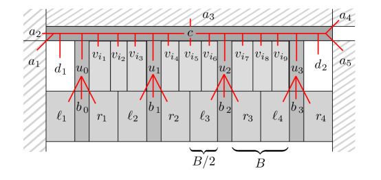
Figure 2: Given an instance $S$ of 3-Partition, we construct a tree $T_{S}$ (thick red line segments) and define boxes such that $T_{S}$ has a realization if and only if $S$ is feasible.

We claim that an instance $S$ of 3-Partition is feasible if and only if $T_{S}$ can be realized with the given box sizes. It is easy to see that $T_{S}$ can be realized if $S$ is feasible: we simply partition vertices $v_{1},\dots,v_{n}$ into groups of three (by vertices $u_{0},\dots,u_{m}$) in the same way as their widths $s_{1},\dots,s_{n}$ are partitioned in groups of three; see Fig. 2.

For the other direction, consider any realization of $T_{S}$. By abusing notation, we refer to the box of some vertex $v$ also as $v$. Since $c$ touches the five large squares $a_{1},\dots,a_{5}$, at least three sides of $c$ are partially covered by some $a_{k}$ and at least one horizontal side of $c$ is completely covered by some $a_{k}$. Since $c$ has height 1/2 only, but touches all the $v_{i}$’s and $u_{j}$’s and $d_{1}$ and $d_{2}$ (each of height $B>1$), all these boxes must touch $c$ on its free horizontal side, say, the bottom side. Furthermore, the sum of the widths of the boxes exactly matches the width of $c$; so they must pack side by side in some order.

This means that the only free boundary of $u_{j}$ is at the bottom, and $u_{j}$ must make contact there with $b_{j}$, $\ell_{j}$, and $r_{j}$. This is only possible if $b_{j}$ is placed directly beneath $u_{j}$, and $\ell_{j}$ and $r_{j}$ make contact with the bottom corners of $u_{j}$. (They need not appear to the left and right as shown in Fig. 2.) Because the sum of the widths of the $b_{j}$’s, $\ell_{j}$’s, and $r_{j}$’s exactly matches the width of $c$, they must pack side by side, and therefore the $u_{j}$’s are spaced distance $B$ apart. There is a gap of width $B/2$ before the first $u_{j}$ and after the last $u_{j}$. These gaps are too wide for one box in $v_{1},\ldots,v_{n}$ and too small for two of them since their widths are contained in the open interval $(B/4,B/2)$. Therefore, the boxes $d_{1}$ and $d_{2}$ must occupy these gaps, and the boxes $v_{1},\ldots,v_{n}$ are packed into $m$ groups each of width $B$, as required. ∎

Note that the proof of the weak NP-hardness for stars still works in case rectangles may be rotated because all boxes are squares—but one. The same holds for the strong NP-hardness for trees; for details see Appendix A.

Although CROWN is NP-hard in general, there are graph classes for which the problem can be solved efficiently. In the remainder of this section, we investigate such a class—irreducible triangulations—, and we consider a restricted variant of CROWN: Hier-CROWN.

2.1 The CROWN problem on irreducible triangulations

A box representation is called a rectangular dual if the union of all rectangles is again a rectangle whose boundary is formed by exactly four rectangles. A graph $G$ admits a rectangular dual if and only if $G$ is planar, internally triangulated, has a quadrangular outer face and does not contain separating triangles [BGPV08]. Such graphs are known as irreducible triangulations. The four outer vertices of an irreducible triangulation are denoted by $v_{N}$, $v_{E}$, $v_{S}$, $v_{W}$ in clockwise order around the outer quadrangle. An irreducible triangulation $G$ may have exponentially many rectangular duals. Any rectangular dual of $G$, however, can be built up by placing one rectangle at a time, always keeping the union of the placed rectangles in staircase shape.

Theorem 2.

CROWN on irreducible triangulations can be solved in linear time.

sketch.

The algorithm greedily builds up the supporting graph $G$, similarly to an algorithm for edge-proportional rectangular duals [NPR13]. We define concavity as a point on the boundary of the so-far constructed representation, which is a bottom-right or top-left corner of some rectangle. Start with a vertical and a horizontal ray emerging from the same point $p$, as placeholders for the right side of $v_{W}$ and the top side of $v_{S}$, respectively. Then at each step consider a concavity, with $p$ as the initial one. Since each concavity $p$ is contained in exactly two rectangles, there exists a unique rectangle $R_{p}$ that is yet to be placed and has to touch both these rectangles. If by adding $R_{p}$ we still have a staircase shape representation, then we do so. If no such rectangle can be added, we conclude that $G$ is not realizable; see Fig. 3. The complete proof is in the appendix. ∎

(a)

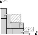
(b)

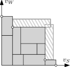
(c)

Figure 3: Left: starting configuration with rays $v_{S}$ and $v_{W}$. Center: representation at an intermediate step: vertex $w$ fits into concavity $p$ and results in a staircase, vertex $v$ fits into concavity $s$ but does not result in a staircase. Adding box $w$ to the representation introduces a new concavity $q$ and allows wider boxes to be placed at $r$. Right: no box can be placed, so the algorithm terminates.

2.2 The Hier-CROWN problem

The Hier-CROWN problem is a restricted variant of the CROWN problem that can be used to create word clouds with a hierarchical structure; see Fig. 1. The input is a directed acyclic graph $G$ with only one sink and with a plane embedding. The task is to find a representation that hierarchically realizes $G$, meaning that for each directed edge $(v,u)$ in $G$ the top of the box for $v$ is in contact with the bottom of the box for $u$.

If the embedding of $G$ is not fixed, the problem is NP-hard even for a tree, by an easy adaptation of the proof of Theorem 1. (Remove the vertices $a_{2},a_{3},a_{4}$, and orient the remaining edges of $T_{S}$ upward according to the representation shown in Fig. 2.) However, if we fix the embedding of the supporting graph $G$, then Hier-CROWN can be solved efficiently.

Theorem 3.

Hier-CROWN can be solved in polynomial time.

Proof.

Let $G$ be the given supporting graph, with vertices corresponding to boxes $B_{1},\ldots,B_{n}$ where $B_{i}$ has height $h_{i}$ and width $w_{i}$, and $B_{1}$ is the unique sink. We first check that the orientation and embedding of $G$ are compatible, that is, that incoming edges and outgoing edges are consecutive in the cyclic order around each vertex.

The main idea is to set up a system of linear equations for the $x$- and $y$-coordinates of the sides of the boxes. Let variables $t_{i}$ and $b_{i}$ represent the $y$-coordinates of the top and bottom of $B_{i}$ respectively, and variables $\ell_{i}$ and $r_{i}$ represent the $x$-coordinates of the left and right of $B_{i}$ respectively. For each $i=1,\dots,n$, impose the linear constraints $t_{i}=b_{i}+h_{i}$ and $r_{i}=\ell_{i}+w_{i}$. For each directed edge $(B_{i},B_{j})$, impose the constraints $t_{i}=b_{j},r_{i}>\ell_{j}$, and $r_{j}>\ell_{i}$. The last two constraints force $B_{i}$ and $B_{j}$ to share some $x$-range in which they can make vertical contact. Initialize $t_{1}=0$.

With these equations, variables $t_{i}$ and $b_{i}$ are completely determined since every box $B_{i}$ has a directed path to $B_{1}$. Furthermore, the values for $t_{i}$ and $b_{i}$ can be found using a depth-first-search of $G$ starting from $B_{1}$.

The $x$-coordinates are not yet determined and depend on the horizontal order of the boxes, which can be established as follows. We scan the boxes from top to bottom, keeping track of the left-to-right order of boxes intersected by a horizontal line that sweeps from $y=0$ downwards. Initially the line is at $y=0$ and intersects only $B_{1}$. When the line reaches the bottom of a box $B$, we replace $B$ in the left-to-right order by all its predecessors in $G$, using the order given by the plane embedding. In case multiple boxes end at the same $y$-coordinate, we make the update for all of them. Whenever boxes $B_{a}$ and $B_{b}$ appear consecutively in the left-to-right order, we impose the constraint $r_{a}\leq\ell_{b}.$

The scan can be performed in $O(n\log n)$ time using a priority queue to determine which boxes in the current left-to-right order have maximum $b_{i}$ value. The resulting system of equations has size $O(n)$ (because the constraints correspond to edges of a planar graph). It is straightforward to verify that the system of equations has a solution if and only if there is a representation of the boxes that hierarchically realizes $G$. The constraints define a linear program (LP) and can be solved efficiently. (A feasible solution can be found faster than with an LP, but we omit the details in this paper.) ∎

We can show that Hier-CROWN becomes weakly NP-complete if rectangles may be rotated, by a simple reduction from Subset Sum (details in Appendix A.2).

3 The Max-CROWN problem

In this section, we study approximation algorithms for Max-CROWN and consider an extremal variant of the problem.

3.1 Approximation Algorithms.

We present approximation algorithms for Max-CROWN restricted to certain graph classes. Our basic building blocks are an approximation algorithm for stars and an exact algorithm for cycles. Our general technique is to find a collection of disjoint stars or cycles in a graph. We begin with stars, using a reduction to the Maximum Generalized Assignment Problem (GAP) defined as follows: Given a set of bins with capacity constraints and a set of items that may have different sizes and values in each bin, pack a maximum-value subset of items into the bins. It is known that the problem is NP-hard (Knapsack and Bin Packing are special cases of GAP), and there exists an $(1-1/e)$-approximation algorithm [FGMS11]. In the remainder, we assume that there is an $\alpha$-approximation algorithm for GAP, setting $\alpha=1-1/e>0.632$.

Theorem 4.

There exists an $\alpha$-approximation algorithm for Max-CROWN on stars.

Proof.

Let $B_{0}$ denote the box corresponding to the center of the star. In any optimal solution for the Max-CROWN problem there are four boxes $B_{1},B_{2},B_{3},B_{4}$ whose sides contain one corner of $B_{0}$ each. Given $B_{1},B_{2},B_{3},B_{4}$, the problem reduces to assigning each remaining box $B_{i}$ to one of the four sides of $B_{0}$, where it makes contact for its whole length; see Fig. 4.

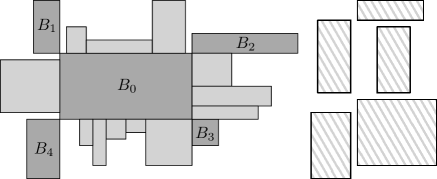
Figure 4: An optimal representation for the Max-CROWN problem whose supporting graph is a star with center $B_{0}$. The striped boxes did not fit into the solution.

This is a special case of GAP: The bins are the four sides of $B_{0}$, the size of an item is its width for the horizontal bins and its height for the vertical bins, and the value of an item is the profit of its adjacency to the central box. We can now apply the algorithm for the GAP problem, which gives an $\alpha$-approximation for the set of boxes. To get an approximation for the Max-CROWN problem, we consider all possible ways of choosing boxes $B_{1},B_{2},B_{3},B_{4}$, which increases the runtime only by a polynomial factor. ∎

In the case where rectangles may be rotated by $90^{\circ}$, the Max-CROWN problem on a star reduces to an easier problem, the Multiple Knapsack Problem, where every item has the same size and value no matter which bin it is placed in. This is because we will always attach a rectangle $B$ to the central rectangle of the star using the smaller dimension of $B$. There is a PTAS for Multiple Knapsack [CK05]. Therefore, there is a PTAS for Max-CROWN on stars if we may rotate rectangles.

A star forest is a disjoint union of stars. Theorem 4 applies to a star forest since we can combine the solutions for the disjoint stars.

Theorem 5.

Max-CROWN on the class of graphs that can be partitioned in polynomial time into $k$ star forests admits an $\alpha/k$-approximation algorithm.

Proof.

The algorithm is to partition the edges of the supporting graph into $k$ star forests, apply the approximation algorithm of Theorem 4 to each star forest, and take the best of the $k$ solutions. This takes polynomial time. We claim this gives the desired approximation factor. Consider an optimum solution, and let $W_{\mathrm{\!opt}}$ be the total profit of edges that are realized as contacts. By the pigeon hole principle, there is a star forest $F$ in the partition with realized profit at least $W_{\mathrm{\!opt}}/k$ in the optimum solution. Therefore our approximation achieves at least $\alpha W_{\mathrm{\!opt}}/k$ profit for $F$. ∎

Corollary 1.

Max-CROWN admits

• an $\alpha/2$-approximation algorithm on trees,

• an $\alpha/5$-approximation algorithm on planar graphs.

Proof.

It is easy to partition any tree into two star forests in linear time. Moreover, it is known that every planar graph has star arboricity at most $5$, that is, it can be partitioned into at most $5$ star forests, and such a partition can be found in polynomial time [HMS96]. The results now follow directly from Theorem 5. ∎

Our star forest partition method is possibly not optimal. Nguyen et al. [NSH⁺08] show how to find a star forest of an arbitrary weighted graph carrying at least half of the profits of an optimal star forest in polynomial-time. We can’t, however, guarantee that the approximation of the optimal star forest carries a positive fraction of the total profit in an optimal solution to Max-CROWN. Hence, approximating Max-CROWN for general graphs remains an open problem. As a first step into this direction, we present a constant-factor approximation for supporting graphs with bounded maximum degree. First we need the following lemma.

Lemma 1.

Given a sequence of $n\geq 3$ boxes, we can find a representation realizing the $n$-cycle in linear time.

Proof.

Let $C=(v_{1},v_{2},\ldots,v_{n})$ be a cycle. Let $W$ be the sum of all the widths, $W=\sum_{i}w_{i}$, and let $t$ be maximum index such that $\sum_{i\leq t}w_{i}<W/2$. We place $v_{1},v_{2},\ldots,v_{t}$ side by side in order from left to right with their bottoms on a horizontal line $h$. We call this the “top channel”. Starting from the same point on $h$ we place $v_{n},v_{n-1},\ldots,v_{t+2}$ side by side in order from left to right with their tops on $h$. We call this the “bottom channel”. Note that $v_{1}$ and $v_{n}$ are in contact. It remains to place $v_{t+1}$ in contact with $v_{t}$ and $v_{t+2}$. It is easy to show that the following works: add $v_{t+1}$ to the channel of minimum width, or in case of a tie, place $v_{t}$ straddling the line $h$. ∎

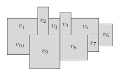
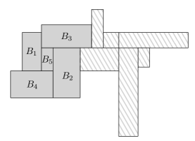
Figure 5: Left: Realizing cycle $(v_{1},\ldots,v_{10})$. Right: $8$ adjacencies with $5$ boxes in Theorem 7.

Following the idea of Theorem 5, we can approximate Max-CROWN by applying Lemma 1 to a partition of the supporting graph into sets of disjoint cycles.

Theorem 6.

Max-CROWN on the class of graphs that can be partitioned into $k$ sets of disjoint cycles (in polynomial time) admits a (polynomial-time) algorithm that achieves total profit at least $\frac{1}{k}\sum_{i\neq j}p_{ij}$. In particular, there is a $1/k$-approximation algorithm for Max-CROWN on this graph class.

Corollary 2.

Max-CROWN on graph of maximum degree $\Delta$ admits a $2/(\Delta+1)$-approximation.

Proof.

As Peterson [Pet91] shows, the edges of any graph of maximum degree $\Delta$ can be covered by $\lceil\Delta/2\rceil$ sets of cycles, and such sets can be found in polynomial time. The result now follows from Theorem 6. ∎

3.2 An Extremal Max-CROWN Problem.

In the following, we bound the maximum number of contacts that can be made when placing $n$ boxes. It is easy to see that for $n=2,3$ any set of boxes allows $2n-3$ contacts. In case $n=4$ the boxes can be arranged so that their corners meet at a point, thus realizing $2n-2$ contacts. For larger $n$ we have:

Theorem 7.

For $n\geq 5$ and any set of $n$ boxes, the boxes can be placed in the plane to realize $2n-2$ contacts. For some sets of boxes this is the best possible.

Proof.

Let $B_{1},\ldots,B_{n}$ be any set of boxes. We place the first 5 boxes to make 8 contacts, and place the remaining boxes to make 2 contacts each for a total of $8+2(n-5)=2n-2$ contacts. Among the first 5 boxes, let $B_{1}$ and $B_{2}$ be the boxes with largest height, and $B_{3}$ and $B_{4}$ be the boxes with largest width. Place the five boxes as in Fig. 5. Place the remaining boxes one by one as in the proof of Lemma 1 along the horizontal line between $B_{2}$ and $B_{3}$. Then each remaining box makes two new contacts.

Next we describe a set of $n$ boxes for which the maximum number of contacts is $2n-2$. Let $B_{i}$ be a square box of side length $2^{i}$. Consider any placement of the boxes and partition the contacts into horizontal and vertical contacts. Here we assume that a point contact of two boxes is horizontal if the point is the south-west corner of the first box and the north-east corner of the second; otherwise, a point contact is vertical. From the side lengths of boxes, it follows that neither set of contacts contains a cycle. Thus each set of contacts has size at most $n-1$ for a total of $2n-2$. ∎

4 The Area-CROWN problem

The same supporting graph can often be realized by different contact representations, not all of which are equally useful or visually appealing when viewed as word clouds. In this section we consider the Area-CROWN problem and show that finding a “compact” representation that fits into a small bounding box is another NP-hard problem.

The reduction is from the (strongly) NP-hard $2$D Strip Packing problem [LMM02]: The input is a set $R$ of $n$ rectangles with height and weight functions $w:R\rightarrow\mathbb{N}$ and $h:R\rightarrow\mathbb{N}$, and a strip of width $W$ and height $H$. All the input numbers are bounded by some polynomial in $n$. The task is to pack the given rectangles into the strip.

The Strip Packing problem is actually equivalent to Area-CROWN when the supporting graph is an independent set. However, edges in the supporting graph impose additional constraints on the representation, which might make Area-CROWN easier. The following theorem (proved in the appendix) shows that this is not the case.

Theorem 8.

Area-CROWN is NP-hard even on paths.

5 Experimental Results

We implemented our new methods for constructing word clouds: the Star Forest algorithm based on extracting star forests (Corollary 1), and the Cycle Cover algorithm based on decomposing edges of a graph into cycle covers (Theorem 6). We compared the algorithms with the existing method from [VWF09] (referred to as Random), the algorithm from [CWL⁺10] (referred to as CPDWCV), and the algorithm from [WPW⁺11] (referred to as Seam Carving). Our dataset is 120 Wikipedia documents, with 400 words or more. For the word clouds, we removed stop-words (e.g., “and”, “the”, “of”), and constructed supporting graphs $G_{50}$ and $G_{100}$ for $50$ and $100$ the most frequent words respectively. Implementation details are provided in the appendix.

We compare the percentage of realized profit in the representation of the supporting graphs. Since Star Forest handles planar supporting graphs, we first extract a maximal planar subgraph of $G$, and then apply the algorithm on the subgraph. The percentage of realized profit is presented in the table. Our results indicate that, in terms of the realized profit, Cycle Cover and Star Forest outperform existing approaches; see Fig. 8. In practice, Cycle Cover realizes more than $17\%$ of the total profit of graphs with $50$ vertices. On the other hand, existing algorithms may perform better in terms of compactness, aspect ratio, and other aesthetic criteria; we leave a deeper comparison of word cloud algorithms as a future research direction.

Algorithm	Realized Profit of $G_{50}$	Realized Profit of $G_{100}$
Random [VWF09]	$3.4\%$	$2.2\%$
CPDWCV [CWL+10]	$12.2\%$	$8.9\%$
Seam Carving [WPW+11]	$7.4\%$	$5.2\%$
Star Forest	$11.4\%$	$8.2\%$
Cycle Cover	$17.8\%$	$13.8\%$

6 Conclusions and Future Work

We formulated the Word Rectangle Adjacency Contact (CROWN) problem, motivated by the desire to provide theoretical guarantees for semantics-preserving word cloud visualization. We described efficient algorithms for variants of CROWN, showed that some variants are NP-hard, and presented several approximation algorithms. A natual open problem is to find an approximation algorithm for general graphs with arbitrary profits.

Acknowledgments. Work on this problem began at Dagstuhl Seminar 12261. We thank the organizers, participants, Therese Biedl, Steve Chaplick, and Günter Rote.

Appendix

Appendix A The CROWN problem

Theorem 1 still holds in the case where rectangles may be rotated. The construction uses squares for the $a_{i}$’s. Rectangle $c$ has height 1/2 and all the other rectangles have both width and height greater than 1/2 so no rectangle can make contact along the sides of $c$ in-between the $a_{k}$’s. Finally, all rectangles have height greater than width, so there is no advantage to rotating any rectangle.

A.1 The CROWN problem on irreducible triangulations

Theorem 2.

CROWN on irreducible triangulations can be solved in linear time.

Proof.

Let $G$ be the supporting graph, an irreducible triangulation. We consider $G$ embedded in the plane with outer face $\{v_{N},v_{E},v_{S},v_{W}\}$. Note that this embedding is unique. By abusing notation, we refer to a vertex and its corresponding box with the same letter.

We begin by placing a horizontal and a vertical ray emerging from the same point in positive $x$-direction and positive $y$-direction, respectively. For the first phase of the algorithm let us pretend that the horizontal ray is the box $v_{S}$ (imagine a rectangle with tiny height and huge width) and the vertical ray is the box $v_{W}$ (imagine a rectangle with tiny width and huge height), independent of how the actual boxes look like; see Fig. 3.

We build up a representation by adding one rectangle at a time. At every intermediate step the representation is rectilinear convex, that is, its intersection with any horizontal or vertical line is connected. In other words, the representation has no holes and a “staircase shape”. We maintain the set of all concavities, that is, points on the boundary of the representation, which are bottom-right or top-left corners of some rectangle but not a top-right corner of any rectangle. Initially there is only one concavity, namely the point where the rays $v_{W}$ and $v_{S}$ meet.

Each concavity $p$ is a point on the boundary of two rectangles, say $u$ and $v$. Since $G$ has no separating triangles there are exactly two vertices that are adjacent to both, $u$ and $v$, or only one if $\{u,v\}=\{v_{S},v_{W}\}$. For exactly one of the these vertices, call it $w$, the rectangle is not yet placed because its bottom-left corner is supposed to be placed on the concavity $p$. We say that $w$ fits into the concavity $p$. We call a vertex $w$ applicable to an intermediate representation if it fits into some concavity and adding the rectangle $w$ gives a representation that is rectilinear convex. In the very beginning the unique common neighbor of $v_{S}$ and $v_{W}$ is applicable.

The algorithm proceeds in $n-4$ steps as follows. At each step we identify a inner vertex $w$ of $G$ that is applicable to the current representation. We add the rectangle $w$ to the representation and update the set of concavities and applicable vertices. At most two points have to be added to the set of concavities, while one is removed from this set. The vertices that fit into the new concavities can easily be read off from the plane embedding of $G$. Checking whether these vertices are applicable is easy. If the top-left or bottom-right corner of $w$ does not define a concavity then one has to check whether the vertices that fit into existing concavities to the left or below, respectively, are now applicable. So each step can be done in constant time.

If the algorithm has placed the last inner vertex, it suffices to check whether the representation without the two rays is a rectangle, that is, whether there are exactly two concavities left. If so, call this rectangle $R$, we check whether the width of $R$ is at most the width of $v_{N}$ and $v_{S}$ and whether the height of $R$ is at most the height of $v_{E}$ and $v_{W}$. If this holds true, we can easily place the rectangles $v_{N}$, $v_{E}$, $v_{S}$, $v_{W}$ to get a representation that realizes $G$. The total running time is linear.

On the other hand, if the algorithm stops because there is no applicable vertex, or the height/width-conditions in the end phase are not met, then there is no representation that realizes $G$. This is due to the lack of choice in building the representation – if a vertex $v$ is applicable to a concavity $p$ then the bottom-left corner of $v$ has to be placed at $p$ in order to establish the contacts of $v$ with the two rectangles containing $p$. ∎

A.2 The Hier-CROWN problem

We justify the claim that Hier-CROWN becomes weakly NP-complete if rectangles may be rotated. We use a reduction from Subset Sum. Given an instance of Subset Sum consisting of $n$ items $s_{i},i=1,\ldots,n$ and a desired sum $S$, construct a large top square $T$ and a large bottom square $B$, and a square $M$ of side-length $n+S$ that must lie between $B$ and $T$. Add a chain of rectangles $B_{1},\ldots,B_{n}$ from $B$ to $T$ where $B_{i}$ has dimensions $1\times(1+s_{i})$. Rectangles $B_{i}$ that are oriented to have height $1+s_{i}$ correspond to “chosen” elements for the Subset Sum problem. Via this correspondence, the Subset Sum instance has a solution if and only if the constructed Hier-CROWN instance has a solution.

Appendix B The Area-CROWN problem

Theorem 8.

Area-CROWN is NP-hard even on paths.

Proof.

We use a reduction from Strip Packing, so fix any instance $I$ of Strip Packing consisting of rectangles $r_{1},\ldots,r_{n}$ and two integers $H$ and $W$. Let $d={\epsilon}/{\max(W,H)}$ for some $\epsilon\in(0,1)$.

We define an instance of the Area-CROWN problem by slightly increasing the heights and widths in $I$. The idea is to lay a unit square grid over the strip and blow each grid line up to have a thickness of $d$; see Fig. 6. Each rectangle in $I$ is stretched according to the number of grid lines is intersects.

(a)

(b)

Figure 6: Grid before and after stretching

More precisely, we define for $i=1,\ldots,n$ a rectangle $r^{\prime}_{i}$ of width $w(r_{i})+(w(r_{i})-1)d$ and height $h(r_{i})+(h(r_{i})-1)d$. Further we define $W^{\prime}=W+(W-1)d$ and $H^{\prime}=H+(H-1)d$. Finally, we arrange the rectangles $r^{\prime}_{1},\ldots,r^{\prime}_{n}$ into a path $P$ by introducing between $r_{i}$ and $r_{i+1}$ ($i=1,\ldots,n-1$), as well as before $r^{\prime}_{1}$ $k$ small $x\times x$ square, called connector squares. We choose $k$ and $x$ to satisfy

$$kx =4(n+3)(H+2nW)\hskip 40.00006pt\text{and}$$ (1)

$$n(kx^{2}+2x) =d.$$ (2)

In particular, we choose

$$x =\frac{d}{2n(2Hn+6H+4n^{2}W+12nW+1)}\hskip 40.00006pt\text{and}$$

$$k =\frac{4(n+3)(H+2nW)}{x}.$$

We claim that there is a representation realizing $P$ within the $W^{\prime}\times H^{\prime}$ bounding box if and only if the original rectangles $r_{1},\ldots,r_{n}$ can be packed into the original $W\times H$ bounding box.

First consider any representation realizing $P$ within the $W^{\prime}\times H^{\prime}$ bounding box and remove all connector squares from it. Since $W^{\prime}<W+\epsilon<W+1$ and $H^{\prime}<H+\epsilon<H+1$, the stretched bounding box has the same number of grid lines than the original. Hence the rectangles $r^{\prime}_{1},\ldots,r^{\prime}_{n}$ can be replaced by the corresponding rectangles $r_{1},\ldots,r_{n}$ and perturbed slightly such that every corner lies on a grid point. This way we obtain a solution for the original instance of Strip Packing.

Now consider any solution for the Strip Packing instance, that is, any packing of the rectangles $r_{1},\ldots,r_{n}$ within the $W\times H$ bounding box. We will construct a representation realizing the path $P$ within the $W^{\prime}\times H^{\prime}$ bounding box. We start blowing up the grid lines of the $W\times H$ bounding box to thickness $d$ each, which also effects all rectangles intersected by a grid line in its interior. This way we obtain a placement of bigger rectangles $r^{\prime}_{1},\ldots,r^{\prime}_{n}$ $I^{\prime}$ in the bigger $W^{\prime}\times H^{\prime}$ bounding box, such that every rectangle $r^{\prime}_{i}$ intersects the interiors of exactly those blown-up grid lines corresponding to the grid lines that intersect $r_{i}$ interiorly. Thus any two rectangles $r^{\prime}_{i}$ and $r^{\prime}_{j}$ are separated by a vertical or horizontal corridor of thickness at least $d$. We will refer to the grid lines of thickness $d$ as gaps.

It remains to place all the connector square so as to realize the path $P$. The idea is the following. We start in the lower left corner of the bounding box, and lay out connector squares horizontally to the right inside the bottommost horizontal gap until we reach the vertical gap that contains the lower-left corner of $r^{\prime}_{1}$. We then start laying out the connector squares inside this vertical gap upwards, until we reach the lower-left corner of $r^{\prime}_{1}$. Whenever a rectangle $r^{\prime}_{i}$ overlaps with this vertical gap, we go around $r^{\prime}_{i}$; see Fig. 7d. This way we lay out at most $(3W^{\prime}+H^{\prime})/x$ connector squares, which by (1) is less than $k$. The remaining connector squares are “folded up” inside the vertical gap; see Fig. 7b.

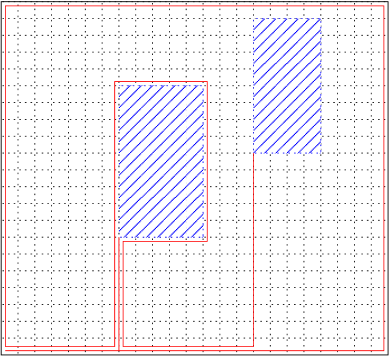
(a) NP-hardness of Area-CROWN for paths

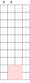
(b) folding connector rectangles inside a gap

(c) connectors before rerouting

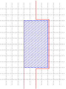
(d) connectors after rerouting

Figure 7: Illustrations for Theorem 8.

Next we lay out the connectors squares between $r^{\prime}_{1}$ and $r^{\prime}_{2}$. We start where we ended before, that is, at the lower-left corner of $r^{\prime}_{1}$, and go the along the path we took before till we reach the bottommost gap. Then we lay connector squares along the outermost gaps in counterclockwise direction, that is, first horizontally to the rightmost gap, then up to the topmost gap, left to the leftmost gap, and down to the bottommost gap. Now we do the same for $r^{\prime}_{2}$ than what we did for $r^{\prime}_{1}$. If while going right we “hit” the connector squares going up to $r^{\prime}_{1}$, we follow them up, go around $r^{\prime}_{1}$, and go down again. This is possible since there are gaps all around $r^{\prime}_{1}$; see Fig. 7a. Note that the red line of connectors will actually sit on the dashed, expanded grid lines but are drawn next to them for better readability.

We repeat the process for all the rectangles.

We have to show two things: The number of connector squares between two $r^{\prime}_{i}$ and $r^{\prime}_{i+1}$ is large enough so that the length of the string of connectors is sufficient. And that the gaps have sufficient space so that we can fold up the connectors in them.

The first condition is taken care of by equation (1). We divide the path of the connectors in up to $n+3$ parts: The first part $p_{{\text{down}}_{i}}$ is going down from $r^{\prime}_{i}$ to the bottom gap. The second part $p_{\text{circle}}$ that goes around the bounding box in counterclockwise order to the vertical gap containing the lower-left corner of $r^{\prime}_{i+1}$. This part is intercepted by up to $n$ parts $p_{{\text{avoid}}_{k}}$ where we hit a string of connectors going up to another rectangle $r^{\prime}_{k}$ and we have to follow it, go around $r^{\prime}_{k}$ and come down again. The last part $p_{{\text{up}}_{i+1}}$ is going up from the bottom gap to the position of $r^{\prime}_{i+1}$. We will now show that each of these parts has a maximum length of $4(H^{\prime}+2nW^{\prime})$.

The parts $p_{{\text{up}}_{i+1}}$ and $p_{{\text{down}}_{i}}$ have to span the height $H^{\prime}$ at most once, and may encounter all other rectangles $r^{\prime}_{k}$ at most once. Going around any such $r^{\prime}_{k}$ means at most traversing its width twice, which is at most $2W^{\prime}$. Hence each of $p_{{\text{up}}_{i+1}}$ and $p_{{\text{down}}_{i}}$ has a total length of at most $H^{\prime}+2nW^{\prime}<4(H^{\prime}+2nW^{\prime})$. Since every $p_{{\text{avoid}}_{k}}$ exactly follows the $p_{{\text{up}}_{k}}$, then surrounds $r^{\prime}_{k}$ (which has maximum width $W^{\prime}$ and maximum height $H^{\prime}$) and then follows $p_{{\text{down}}_{k}}$, it has a maximum length of $2(W^{\prime}+H^{\prime})+2(H^{\prime}+2nW^{\prime})\leq 4(H^{\prime}+2nW^{\prime})$. Finally, $p_{\text{circle}}$ has a maximum length of $2H^{\prime}+2W^{\prime}\leq 4(H^{\prime}+2nW^{\prime})$.

Thus, the total length of the path of connectors comprised of $n+3$ parts of at most length $4(H^{\prime}+2nW^{\prime})$ each is at most $4(n+3)(H^{\prime}+2nW^{\prime})$. Equation (1) ensures that our string of connectors has sufficient length.

The second condition is covered by equation (2). Consider Fig. 7b. If a string of connectors just passes through a gap, it takes up exactly $1\times x$ space. If it folds $m$ connector rectangles inside the gap, it takes $m\times x^{2}$ plus the ’wasted’ space (the red shaded space in Fig. 7b). The wasted space can be at most $1\times 2x$, and since every string of connectors has $k$ connector rectangles, the space taken up by those can be at most $kx^{2}$, thus every string of connectors can take at most $kx^{2}+2x$ space in any given gap. Since there are $n$ such strings of connectors and every gap has dimensions $1\times d$, equation (2) ensures that the space in every gap is sufficient.

We showed that we can find a layout of the path that corresponds to the optimum packing of the rectangles, if such a packing exists within the desired bounding box. Thus, finding the most space-efficient layout for a path of rectangles is NP-hard. ∎

Appendix C Experimental Results

Here we provide some details regarding the implementation of the algorithms.

Before the algorithms are applied, the text is preprocessed using this workflow: The text is split into sentences, and the sentences are split into words using Apache OpenNLP. We then remove stop words, perform stemming on the words and group the words with the same stem. The similarity of words is computed using Latent Semantic Analysis based on the co-occurrence of the words within the same sentence.

In the implementation of Star Forest, we use the $(\frac{\beta}{\beta+1}-\epsilon)$-approximation of Fleischer et al. [FGMS11] combined with a FPTAS for Knapsack to approximate the stars. In the implementation of CPDWCV, we achieved the best results in our experiments with parameters $K_{r}=1000$ and $K_{a}=25$. Some results are given in Fig. 8.

(a) Random Layout

(b) Seam Carving ([WPW⁺11])

(c) CPDWCV ([CWL⁺10])

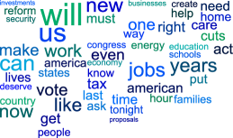
(d) Star Forest (Corollary 1)

(e) Cycle Cover (Corollary 2)

Figure 8: Word clouds generated for Obama’s 2013 State of the Union Speech by various algorithms. Percentage of the total realized profit: (a) $2.3\%$ (b) $7.1\%$ (c) $11.8\%$ (d) $12.7\%$ (e) $18.2\%$

The experiments have been run on an Intel i5 3.2GHz with 8GB RAM. The Random, Star Forest, and Cycle Cover algorithms finishes in under a second. The CPDWCV and Seam Carving algorithms are based on a force-directed model, and compute the word cloud with $100$ words within several seconds.

References

- [BGPV08] Adam L. Buchsbaum, Emden R. Gansner, Cecilia Magdalena Procopiuc, and Suresh Venkatasubramanian. Rectangular layouts and contact graphs. ACM Transactions on Algorithms, 4(1), 2008.
- [CK05] C. Chekuri and S. Khanna. A polynomial time approximation scheme for the multiple knapsack problem. SIAM Journal on Computing, 35(3):713–728, 2005.
- [CVW09] Christopher Collins, Fernanda B. Viégas, and Martin Wattenberg. Parallel tag clouds to explore and analyze faceted text corpora. In IEEE VAST, pages 91–98, 2009.
- [CWL+10] W. Cui, Y. Wu, S. Liu, F. Wei, M. X. Zhou, and H. Qu. Context-preserving, dynamic word cloud visualization. Computer Graphics and Applications, 30:42–53, 2010.
- [DMS05] Tim Dwyer, Kim Marriott, and Peter J. Stuckey. Fast node overlap removal. In 13th Symposium on Graph Drawing, volume 3843 of LNCS, pages 153–164, 2005.
- [EMSV12] David Eppstein, Elena Mumford, Bettina Speckmann, and Kevin Verbeek. Area-universal and constrained rectangular layouts. SIAM Journal on Computing, 41(3):537–564, 2012.
- [Fel13] Stefan Felsner. Rectangle and square representations of planar graphs. In Thirty Essays on Geometric Graph Theory, pages 213–248. Springer, 2013.
- [FGMS11] Lisa Fleischer, Michel X. Goemans, Vahab S. Mirrokni, and Maxim Sviridenko. Tight approximation algorithms for maximum separable assignment problems. Math.Op.R., 36(3):416–431, 2011.
- [Fus09] Éric Fusy. Transversal structures on triangulations: A combinatorial study and straight-line drawings. Discrete Mathematics, 309(7):1870–1894, 2009.
- [GH10] Emden R. Gansner and Yifan Hu. Efficient, proximity-preserving node overlap removal. J. Graph Algorithms Appl., 14(1):53–74, 2010.
- [GJ79] Michael R. Garey and David S. Johnson. Computers and Intractability: A Guide to the Theory of NP-Completeness. W. H. Freeman & Co., New York, NY, USA, 1979.
- [HMS96] S.L. Hakimi, J. Mitchem, and E. Schmeichel. Star arboricity of graphs. Discrete Mathematics, 149(1 3):93–98, 1996.
- [KLKS10] Kyle Koh, Bongshin Lee, Bo Hyoung Kim, and Jinwook Seo. Maniwordle: Providing flexible control over Wordle. IEEE Trans. Vis. Comput. Graph., 16(6):1190–1197, 2010.
- [LHKK96] Krista Lagus, Timo Honkela, Samuel Kaski, and Teuvo Kohonen. Self-organizing maps of document collections: A new approach to interactive exploration. In KDD, pages 238–243, 1996.
- [LMM02] Andrea Lodi, Silvano Martello, and Michele Monaci. Two-dimensional packing problems: A survey. European Journal of Operational Research, 141(2):241–252, 2002.
- [NB12] Arlind Nocaj and Ulrik Brandes. Organizing search results with a reference map. IEEE Transactions on Visualization and Computer Graphics, 18(12):2546–2555, 2012.
- [NPR13] Martin Nöllenburg, Roman Prutkin, and Ignaz Rutter. Edge-weighted contact representations of planar graphs. In Graph Drawing, volume 7704 of LNCS, pages 224–235. Springer, 2013.
- [NSH+08] C Thach Nguyen, Jian Shen, Minmei Hou, Li Sheng, Webb Miller, and Louxin Zhang. Approximating the spanning star forest problem and its application to genomic sequence alignment. SIAM Journal on Computing, 38(3):946–962, 2008.
- [Pet91] Julius Petersen. Die Theorie der regulären Graphen. Acta Mathematica, 15(1):193–220, 1891.
- [Rai34] Erwin Raisz. The rectangular statistical cartogram. Geographical Review, 24(3):292–296, 1934.
- [RT86] Pierre Rosenstiehl and Robert E Tarjan. Rectilinear planar layouts and bipolar orientations of planar graphs. Discrete & Computational Geometry, 1(1):343–353, 1986.
- [Tho86] Carsten Thomassen. Interval representations of planar graphs. Journal of Combinatorial Theory, Series B, 40(1):9–20, 1986.
- [VWF09] Fernanda B. Viégas, Martin Wattenberg, and Jonathan Feinberg. Participatory visualization with Wordle. IEEE Trans. Vis. Comput. Graph., 15(6):1137–1144, 2009.
- [WPW+11] Yingcai Wu, Thomas Provan, Furu Wei, Shixia Liu, and Kwan-Liu Ma. Semantic-preserving word clouds by seam carving. Computer Graphics Forum, 30(3):741–750, 2011.