Anomalous diffusion and response in branched systems: a simple analysis

Abstract

We revisit the diffusion properties and the mean drift induced by an external field of a random walk process in a class of branched structures, as the comb lattice and the linear chains of plaquettes. A simple treatment based on scaling arguments is able to predict the correct anomalous regime for different topologies. In addition, we show that even in the presence of anomalous diffusion, the Einstein’s relation still holds, implying a proportionality between the mean-square displacement of the unperturbed systems and the drift induced by an external forcing.

I Introduction

The Einstein’s work on Brownian motion represents one of brightest example of how Statistical Mechanics Einstein operates by providing the first-principle foundation to phenomenological laws. In his paper, the celebrated relationship between the diffusion coefficient and the Avogadro’s number $N_{A}$ was the first theoretical evidence on the validity of the atomistic hypothesis. In addition, he derived the first example of a fluctuation dissipation relation (FDR) Kubo ; Bettolo08 .

Let $x_{t}$ be the position of a colloidal particle at time $t$ undergoing collisions from small and fast moving solvent particles, in the absence of an external forcing. At large times we have:

$$\langle x_{t}\rangle_{0}=0,\qquad\langle x_{t}^{2}\rangle_{0}\simeq 2D\,t\;,$$ (1)

where $D$ is the diffusion coefficient and the average $\langle\cdots\rangle_{0}$ is over an ensemble of independent realizations of the process. The presence of an external constant force-field $F$ induces a linear drift

$$\langle\delta x_{t}\rangle_{F}=\langle x_{t}\rangle_{F}-\langle x_{t}\rangle_{0}=\mu Ft$$ (2)

where $\langle\cdots\rangle_{F}$ denotes the average over the perturbed system trajectories and $\mu$ indicates the mobility. Einstein was able to prove that the following remarkable relation holds:

$$\frac{\langle x_{t}^{2}\rangle_{0}}{\langle x_{t}\rangle_{F}-\langle x_{t}\rangle_{0}}=\frac{2k_{B}T}{F}\;.$$ (3)

The above equation is an example of a class of general relations known as Fluctuation Dissipation Relations, whose important physical meaning is the following: the effects of small perturbations on a system can be understood from the spontaneous fluctuations of the unperturbed system Kubo ; Bettolo08 .

Anomalous diffusion is a well known phenomenon ubiquitous in Nature anomal_Rev90 ; Castiglione99 ; Klafter_book characterized by an asymptotic mean square displacement behaving as

$$\langle x_{t}^{2}\rangle_{0}\simeq t^{2\nu}\quad\quad\mbox{with~{}}\nu\neq\frac{1}{2}\;.$$ (4)

The case $\nu>1/2$ is called superdiffusive, whereas $\nu<1/2$ corresponds to subdiffusive regimes. The nonlinear behaviour (4) occurs in situations whereby the Central Limit Theorem does not apply to the process $x_{t}$. This happens in the presence of strong time correlations and can be found in chaotic dynamics Geisel84 ; klages_AnTrBook , amorphous materials Amorph and porous media Berkowitz2000 ; Koch88 as well.

Anomalous diffusion is not an exception also in biological contexts, where it can be observed, for instance, in the transport of water in organic tissues kopf1996anomalous ; Tortuosity2 or migration of molecules in cellular cytoplasm Cytoplasm ; Cell_Transp . Biological environments which are crowded with obstacles, compartments and binding sites are examples of media strongly deviating from the usual Einstein’s scenario. Similar situations occur when the random walk (RW) is restricted on peculiar topological structures Ben-Avraham ; Weiss_Comb ; Weiss_Shlomo87 , where subdiffusive behaviours spontaneously arise. In such conditions, it is rather natural to wonder whether the fluctuation-response relationship (3) holds true and, if it fails, what are its possible generalizations.

The goal of this paper is to present a derivation based on a simple physical reasoning, i.e. without sophisticated mathematical formalism, of both the anomalous exponent $\nu$ and Eq. (3) for RWs on a class of comb-like and branched structures Burioni05 consisting of a main backbone decorated by an array of sidebranches as in Fig. 1. Such branched topology is typical of percolation clusters at criticality, which can be viewed as finitely ramified fractals coniglio81 ; coniglio82 . Comb-like structures moreover are frequently observed in condensed matter and biological frameworks: they describe the topology of polymers polycomb ; polybranch , in particular of amphiphilic molecules, and can be also engineered at the nano and microscale. Moreover, they are studied as a simple models for channels in porous media and a general account for these systems can be found in Ref. Ben-Avraham .

Figure 1: Cartoon of a one dimensional lattice (backbone) decorated by identical arbitrary-shaped sidebranches or dead-ends depicted as lateral irregular objects. Such sidebranches act as temporary traps for the random walk along the backbone.

The diffusion along the backbone, longitudinal diffusion, can be strongly influenced by the shape and the size of such branches and anomalous regimes arise by simply tuning their geometrical importance over the backbone. In other words, the dangling lateral structures, dead-ends, introduce a delay mechanism in the hopping to neighbour backbone-sites that easily leads to non Gaussian behaviour, as it was observed for instance in flows across porous media conigliostanley ; Hoffmann_RepSiepCarp .

The simple analysis of the RW on such lattices is based on the homogenization time, meant as the shortest timescale after which the longitudinal diffusion becomes standard. The homogenization time $t_{*}(L)$ can be identified with the typical time taken by the walker to visit most of the $M_{sb}(L)$ sites in a single sidebranch of linear size $L$. Such a time is expected to be a growing function of $M_{sb}(L)$ and thus of $L$: $t_{*}(L)=g[M_{sb}(L)]$. In the following, we shall see how the scaling properties of $t_{*}(L)=g[M_{sb}(L)]$ can be easily extracted from graph-theoretical considerations, in simple and complex structures as well.

Once such a scaling is known, we can apply a “matching argument” to derive the exponent $\nu$ in the relation (4). For finite-size sidebranches indeed, the anomalous regime in the longitudinal diffusion is transient and soon or later it will be replaced by the standard diffusion,

$$\langle x_{t}^{2}\rangle\sim\begin{cases}t^{2\nu}&\mbox{if $t\ll t_{*}(L)$}\\ D(L)\,t&\mbox{if $t\gg t_{*}(L)$}\end{cases}$$ (5)

where $D(L)$ is the effective diffusion coefficients depending on $L$. The power-law and the linear behaviors have to match at time $t\sim t_{*}(L)$, thus we can write the matching condition

$$t_{*}(L)^{2\nu}\sim D(L)\>t_{*}(L)\quad\mbox{or equivalently}\quad t_{*}(L)^{2\nu-1}\sim D(L)\,,$$ (6)

accordingly, both the scaling $D(L)\sim L^{-u}$ and $t_{*}(L)\sim L^{v}$ provide a direct access to the exponent $\nu$ via the expression $(1-2\nu)v=u$. We shall see in the following, how the values of $u$ and $v$ are determined by two relevant dimensions of RW problem: the spectral ($d_{S}$) and the fractal ($d$) dimensions. The former is related to return probability to a given point of the RW and the latter defines the scaling $M_{sb}(L)\sim L^{d}$.

Moreover, we will show that the anomalous regimes observed in branched graphs satisfy the FDR (3) supporting the view that FDR has a larger realm of applicability than Gaussian diffusion, as already pointed out by other authors in similar and different contexts Villamaina011 ; Barkai98 ; Metzler_PhysRep ; Chechkin12 . In the branched systems considered in this work, the generalization of FDR is due to a perfect compensation in the anomalous behaviour of the numerator and the denominator of the ratio (3).

The paper is organized as follows, in sect.2, we discuss the diffusion and the response by starting from the simplest branched structure: the classical comb-lattice (Fig. 2), i.e. a straight line (backbone) intersected by a series of sidebranches. The generalization to more sophisticated ”branched structures” made of complex and fractal sidebranches is reported in sect.3. Sect.4 contains conclusions, where, possible links of the FDRs here derived to other frameworks are briefly discussed.

II The simplest branched structure

At first, we consider the basic model: the simplest comb lattice is a discrete structure consisting of a periodic and parallel arrangement of the “teeth” of length $L$ along a “backbone” line (B), see Fig. 2. This model was proposed by Goldhirsch et al. Goldhirsch_Gefen86 as a elementary structure able to describe some properties of transport in disordered networks and can be well adapted to all physical cases where particles diffuse freely along a main direction but can be temporarily trapped by lateral dead-ends.

Figure 2: Sketch of the simplest comb-lattice structure made of a “backbone” (horizontal array) and “tooth” (lateral arrays) of size $L$.

The walker occupying a site can jump to one of the nearest neighbour sites. Denoting by $\mathbf{r}_{t}=(x_{t},y_{t})$ the position of the walker at time $t$, we can define for the longitudinal displacement from the initial position:

$$x_{t}-x_{0}=\sum_{j=1}^{t}\delta_{j}$$ (7)

where $\{\delta_{j}\}$ are non independent random variables such that

$$\delta_{j}=\left\{\begin{array}[]{ll}\delta^{\parallel}_{j}&\mbox{if ~{}$\mathbf{r}_{j}\in$B}\\ 0&\mbox{if ~{}$\mathbf{r}_{j}\notin$B}\end{array}\right.$$

where $\delta^{\parallel}_{j}=\{-1,0,1\}$ with probability $\{1/4,1/2,1/4\}$ respectively and $B$ denotes the set of points with $y=0$, i.e. forming the backbone B (Fig. 2). A simple algebra yields

$$\langle(x_{t}-x_{0})^{2}\rangle_{0}=\sum_{j=1}^{t}\langle\delta_{j}^{2}\rangle_{0}+2\sum_{j=1}^{t}\sum_{i>j}^{t}\langle\delta_{j}\delta_{i}\rangle_{0}$$

where terms $\langle\delta_{j}^{2}\rangle_{0}=0$ if $\mathbf{r}_{j}\notin$B, whereas $\langle\delta_{j}^{2}\rangle_{0}=1/2$ if $\mathbf{r}_{j}\in$B. On the other hand $\langle\delta_{j}\delta_{i}\rangle_{0}=0$ for all $j\neq i$. Therefore we have

$$\langle(x_{t}-x_{0})^{2}\rangle_{0}=\frac{1}{2}tf_{t}$$ (8)

where $f_{t}$ is the mean percentage of time (frequency) the walker spends in the backbone B during the time interval $[0,t]$. To evaluate $f_{t}$, we begin from the case $t>t_{*}(L)$, $t_{*}(L)$ being the homogenization time, meant as the time taken by the walker to span a whole tooth, visiting at least once all the sites Weissbook . Since along the $y$-direction the one-dimensional diffusion $\langle y_{t}^{2}\rangle\simeq 2D_{0}t$ is fast enough to explore exhaustively the size $L$ and, more importantly, it is recurrent, $t_{*}(L)$ can be taken as the time such that $\langle y_{t}^{2}\rangle\sim L^{2}$ and thus $t_{*}(L)\sim L^{2}$. Since, after the time of the order $t_{*}(L)\sim L^{2}$, the probability for the walker to be in a site of the tooth can be considered to be almost uniform, we have

$$f_{t}=\frac{1}{1+L}\simeq L^{-1},$$

hence for $t\geq t_{*}(L)$, the mean square displacement behaves as

$$\langle(x_{t}-x_{0})^{2}\rangle_{0}\simeq\frac{1}{2(1+L)}t$$ (9)

with an effective diffusion coefficient $D(L)=1/[4(L+1)]$. In the above derivation, we have assumed that the lateral teeth are equally spaced at distance $1$. When the spacing is $\ell>1$ the formula changes to $D(L)=1/[4(L+\ell)]$. This formula can be interpreted as the ratio between the free $D_{0}=1$ and the effective diffusivity $D(L)$. In the literature on transport processes, this ratio is sometimes referred to as tortuosity and it describes the hindrance posed to the diffusion process by a geometrically complex medium in comparison to an environment free of obstacles Tortuosity ; Tortuosity2 .

The diffusion on a simple comb lattice for $L=\infty$ is known to be anomalous Weiss_Comb ; anomal_Rev90 ; Redner . For finite $L$ the diffusion remains anomalous as long as the RW does not feel the finite size of the sidebranches. Therefore for times $t<t_{*}(L)$, we expect an anomalous behaviour

$$\langle(x_{t}-x_{0})^{2}\rangle_{0}\sim t^{2\nu}$$ (10)

where the exponent $\nu$ can be computed by the matching condition (6), with $t_{*}(L)\sim L^{2}$ and $D(L)\sim L^{-1}$, yielding $L^{4\nu}\sim L^{-1}\times L^{2}$, from which $\nu=1/4$,

$$\langle(x_{t}-x_{0})^{2}\rangle_{0}\sim t^{1/2}.$$ (11)

This result can be rigorously derived from standard random walks techniques Weiss_Comb . It is interesting to note that, as the homogenization time $t_{*}(L)$ diverges with the size $L$, upon choosing the appropriate $L$, the anomalous regime can be made arbitrarily long till it becomes the dominant feature of the process.

The longitudinal diffusion is a process determined by the return statistics of the walkers to the backbone. The walker indeed becomes “active” only after a return time $T_{r}=T_{r}(t)$ (operational time) which is actually a stochastic variable of the original discrete clock $t=nt_{0}$. This is an example of subordination: the longitudinal diffusion is subordinated to a simple discrete-time RW through the operational time $T_{r}$. In a more familiar language, we are observing a Continuous Time Random Walk (CTRW) where waiting times are the return times to backbone sites Redner during the motion along the teeth. CTRW on a lattice, proposed by Montroll and Weiss CTRW_latt , is a generalization of the simple RW where jumps among neighbour sites do not occur at regular intervals ($t_{k}=kt_{0}$) but the waiting times between consecutive jumps are distributed according to a probability density $\psi(t)$. Shlesinger Shlesinger74 showed that anomalous diffusion arises if $\psi(t)$ is long tailed.

The equation governing the CTRW is

$$P(x,t)=\sum_{n=0}^{\infty}G(x,n)P(n,t)$$ (12)

where $G(x,n)$ is the probability distribution of the variable $x$ after $n$-steps along the backbone from the origin $x=0$ and $P(n,t)$ indicates the probability to make exactly $n$-steps in the time interval $[0,t]$. The probability $P(n,t)$ is related to the waiting-time distribution $\psi(t)$. On the comb lattice, the waiting-time distribution $\psi(t)$ coincides with the distribution of first-return time to the backbone sites, which for infinite sidebranches is long-tailed and asymptotically decays as $\psi(t)\sim t^{-3/2}$ (see Weiss_Comb ). For finite sidebranches of size $L$, the distribution is truncated to $t_{*}(L)$ by the finite-size effect, thus $\psi(t)\sim t^{-3/2}\exp[-t/t_{*}(L)]$, Refs. anomal_Rev90 and Redner .

We now consider the problem of the response of a driven RW on a comb lattice in the presence of an infinitesimal longitudinal (i.e. parallel to the backbone line) external field $\epsilon$ Villamaina011 ; Giusiano . In that case, the displacement on the backbone is

$$x_{t}-x_{0}=\sum_{j=1}^{t}\Delta_{j}^{(\epsilon)}$$

where

$$\Delta_{j}^{(\epsilon)}=\left\{\begin{array}[]{ll}\delta_{j}^{(\epsilon)}&\mbox{if ~{}$\mathbf{r}_{j}\in$B}\\ 0&\mbox{if ~{}$\mathbf{r}_{j}\notin$B}\end{array}\right.$$

$\delta_{j}^{(\epsilon)}=\{-1,0,1\}$ with probabilities, $\{(1/4+\delta p),1/2,(1/4-\delta p)\}$, so that $\langle\delta_{j}^{(\epsilon)}\rangle=\epsilon$. Thus a biased RW with jumping probabilities $1/4-\delta p$ and $1/4+\delta p$ to the left and to the right respectively is used to model the effect of a static external field. The average jump is $\langle\delta_{j}^{(\epsilon)}\rangle=1\times(1/4+\delta p)-1\times(1/4-\delta p)=2\delta p$, thus $\epsilon=2\delta p$. Notice that $\epsilon$ plays the role of the external field $F$. By the same argument used for the free RW on the comb, we obtain

$$\langle\delta x_{t}\rangle_{\epsilon}=\langle(x_{t}-x_{0})\rangle_{\epsilon}-\langle(x_{t}-x_{0})\rangle_{0}=\epsilon tf_{t}.$$ (13)

The comparison of Eq. (8) and Eq.(13) provides the general result

$$\frac{\langle(x_{t}-x_{0})^{2}\rangle_{0}}{\langle\delta x_{t}\rangle_{\epsilon}}=\frac{1}{2\epsilon}\;.$$ (14)

We stress that this expression holds at any time: for both $t\gtrsim t_{*}(L)$ and $t\lesssim t_{*}(L)$ Villamaina011 , thus it works even when the averages are not taken over the realizations of a Gaussian process. In this respect, Eq. (14) represents a generalization of the Einstein’s relation (14) to the RW over comb lattices in agreement with analogous results found in different systems and contexts Barkai98 ; Metzler_PhysRep ; Chechkin12 .

This property is a simple consequence of the subordination condition expressed by Eq. (12). In fact, the small bias in the left/right jump ($\epsilon=2\delta p$) along the backbone introduces a shift in the distribution of steps

$$G_{\epsilon}(x,n)=\frac{1}{\sqrt{2\pi D_{s}n}}\exp\bigg{[}-\frac{(x-\epsilon n)^{2}}{2D_{s}n}\bigg{]}$$

where $D_{s}=1/2$ is the diffusion coefficient of the subordinated dynamics $D_{s}=\lim_{n\to\infty}\langle({\tilde{x}}_{n}-{\tilde{x}}_{0})^{2}\rangle/(2n)$ and ${\tilde{x}}_{n}$ indicates the position after $n$ jumps on the backbone; for $\epsilon=0$ the distribution is a unbiased Gaussian (in the limit of large $t$ also $n$ is large and the Binomial is well approximated by Gaussian $G_{0}(x,n)$). Actually the precise shape of $G_{\epsilon}(x,n)$ is not very relevant. Since $\langle{\tilde{x}}_{n}\rangle=\epsilon n$ we can compute the biased displacement in the perturbed system

$$\langle x_{t}\rangle_{\epsilon}=\epsilon\sum_{n=0}^{\infty}P(n,t)\;n\;.$$

Considering that $\langle n(t)\rangle=\sum_{n}P(n,t)\;n$, we can re-write

$$\langle x_{t}\rangle_{\epsilon}=\epsilon\langle n(t)\rangle\;.$$

From Eq. (12) we compute the MSD obtaining $\langle x_{t}^{2}\rangle_{0}=\langle n(t)\rangle/2$ which is the same result of Eq. (8), hence Eq. (14) follows. Note that FDR is exact also for anomalous behaviours as the drift we have applied has no effect (or no components) on the sidebranches, therefore the waiting time distribution and thus $P_{n}(t)$ remains unaltered with respect to that of the unperturbed system.

To verify the above results, we generated $N_{p}=7\times 10^{4}$ independent RW trajectories for $t=2\times 10^{7}$ time steps over a regular comb-lattice with different sidebranch sizes $L$.

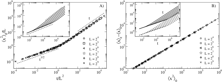
Figure 3: A) rescaled MSD, $\langle x^{2}\rangle_{0}/L$, for the comb lattice (Fig. 2) of tooth length $L$, as a function of the rescaled time $t/L^{2}$. There is a crossover, at $t/L^{2}\sim 1$ (i.e. $t\simeq t_{*}\sim L^{2}$) between a subdiffusive, $t^{1/2}$, to a standard regime $t$. Inset: plot of $\langle x^{2}\rangle_{0}$ vs. $t$ without rescaling for different $L$. B) plot showing the generalized fluctuation-dissipation relation (14). The slope of the dashed straight line is $2\epsilon$, where $\epsilon=2\delta p=0.02$ as prescribed by Eq. (14). Inset: separate plot of MSD and fluctuation $\langle\delta x_{t}\rangle_{\epsilon}$ vs. time to appreciate their common behaviour in both anomalous and standard regime.

Panel A of Fig. 3 refers to the mean square displacement (MSD) for an ensemble of walkers on the traditional comb-lattice (Fig. 2) at different teeth length to probe the homogenization effects characterized by the time $t_{*}(L)\sim L^{2}$. The rescaled data ($t/L^{2}$, $\langle x^{2}\rangle_{0}/L$) collapse onto a master curve showing a clear crossover, at the rescaled crossover time, from a subdiffusive, $t^{1/2}$, to a standard regime, $t$. The response (panel B of Fig. 3) for the same lattice fulfills the generalized fluctuation-dissipation relation (14), thus a plot of the response $\langle x_{t}\rangle_{\epsilon}-\langle x_{t}\rangle_{0}$ vs. the fluctuation $\langle(x_{t}-x_{0})^{2}\rangle_{0}$ shows that the data for different values of $L$ align along a straight line with slope $\epsilon=2\delta p$. The perfect alignment is a consequence of the exact compensation at every time between fluctuations and response (inset of Fig. 3B). In the simulations of Fig. 3B, the drift is implemented by an unbalance $\delta p=0.01$ in the jump probability along the backbone giving $\epsilon=2\delta p=0.02$.

III Generalized branched structures

Interestingly, the previous analysis can be easily extended to the cases where each tooth of the comb is replaced by a more complicated structure, e.g. a two dimensional plaquette, a cube or a even graph with fractal dimension $d$ and spectral dimension $d_{S}$. The spectral dimension is defined by the decay of the return probability $P(t)$ to a generic site in $t$ steps $P(t)\sim t^{-d_{S}/2}$ Ben-Avraham ; Alexander , while the ratio between $d_{S}$ and $d$ is known to control the mean-square displacement behaviour Ben-Avraham

$$\langle x^{2}(t)\rangle\sim t^{d_{S}/d}.$$ (15)

Of course, formula (7) still applies to fractal-like graphs and Eqs. (8,14) hold true, provided an appropriate change in the “geometrical” prefactor is introduced, as we explain in the following.

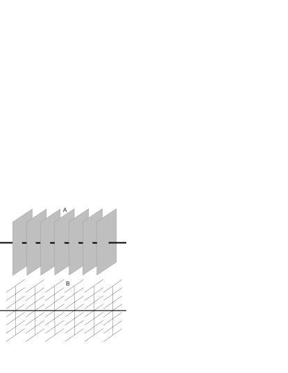
Figure 4: Sketch of the comb structures used in the simulations and obtained as an infinite periodical arrangement of the same geometrical element: A) comb of plaquettes (dubbed “kebab”) and B) two-nested comb lattices (“antenna”).

In the general case where the “teeth” are fractal structures with spectral and fractal dimensions $d_{S}$ and $d$ respectively, the lateral diffusion satisfies

$$\langle y_{t}^{2}\rangle_{0}\sim t^{d_{S}/d}.$$

Here, and in the following, $y_{t}$ indicates the transversal process with respect to the backbone. The previous argument for the homogenization time stems straightforwardly by noting that a walker on an infinite sidebranch, in an interval $t$, visits a number of different sites Alexander ; Weiss_Comb ; Ben-Avraham

$$M_{sb}(t)\sim\left\{\begin{array}[]{ll}t^{d_{S}/2}&\mbox{if $d_{S}\leq 2$}\\ t&\mbox{if $d_{S}>2$}\end{array}\right.\,$$ (16)

and accordingly, in a finite sidebranch of linear size $L$, the homogenization time $t_{*}(L)$ is obtained by the condition $M_{sb}[t_{*}(L)]\sim L^{d}$ of an almost exhaustive exploration of the sites. Then when the sidebranch has spectral dimension $d_{S}\leq 2$, the first condition of (16) yields an homogenization time $t_{*}(L)\sim L^{2d/d_{S}}$ Whereas, if the sidebranch has $d_{S}>2$, the second condition of (16) must be used to obtain $t_{*}(L)\sim L^{d}$. The physical reason of a different expression of $t_{*}(L)$ above and below $d_{S}=2$ is due to the non-recurrence of the RW for $d_{S}>2$ anomal_Rev90 . In this case, the exploration of the sidebranches over a diffusive time scale defined by the law (15) is not significant and the full sampling takes a much longer time which can be estimated directly from the second of Eqs. (16).

Now using Eq. (6), we obtain in the case $d_{S}<2$

$$\langle(x_{t}-x_{0})^{2}\rangle_{0}\sim t^{2\nu},\qquad 2\nu=1-\frac{d_{S}}{2}.$$ (17)

These results coincide with the exact relations obtained by a direct calculation of the spectral dimension on branched structures, based on the asymptotic behavior of the return probability on the graph, or on renormalization techniques Sofia95 ; Burioni05 ; Haynes .

The case $d_{S}=2$ deserves a specific treatment thus, as an example, we consider the ”kebab lattice” (Fig. 4) where each plaquette is a regular two dimensional square lattice, for which $d_{S}=d=2$. Indeed $d_{S}=2$ is the critical dimension separating recurrent ($d_{S}<2$) and not recurrent ($d_{S}>2$) RWs. Thus $d_{S}=2$ is the marginal dimension anomal_Rev90 which reflects into the logarithmic scaling of the transversal MSD $\langle y_{t}^{2}\rangle_{0}\sim t/\ln(t)$, hence the homogenization time is now $t_{*}(L)\sim L^{2}\ln(L)$. Applying once again the matching argument, we obtain the scaling

$$\langle(x_{t}-x_{0})^{2}\rangle_{0}\sim\ln(t)$$ (18)

indicating a logarithmic pre-asymptotic diffusion along the backbone. The time evolution of MSD from initial positions of the simulated random walkers on the “kebab” lattice verifies the transient behaviour (18) at different sizes $L$, Fig. 5A.

Notice that, in our matching arguments, we only make use of the spectral and fractal dimension of the sidebranches. Interestingly, these two parameters are left unchanged if one performs a set of small scale transformations on the graph Univ , without altering their large scale structure. Our results hold therefore true also for different and disordered sidebranches, provided the two dimensions are unchanged.

Following the same steps as those described for the comb lattice, the generalized fluctuation-dissipation relation also holds for all branched structures. To check the result we study the “kebab” lattice (Fig. 4A), where the two-dimensional plaquette is a regular square lattice of side $L_{y}$ and unitary spacing Sofia95 . It follows that:

$$\frac{\langle(x_{t}-x_{0})^{2}\rangle_{0}}{\langle\delta x_{t}\rangle_{\epsilon}}=\frac{1}{3\epsilon},$$ (19)

the prefactor $1/3$ stems from the fact that, in a comb-plaquette lattice, the probability to jump back and forth along the backbone is $1/6$. Panel B of Fig. 5 reports the verification of the fluctuation-dissipation relation: independently of the lattice size, the plot response vs. MSD is a straight line with slope $1/(3\epsilon)$.

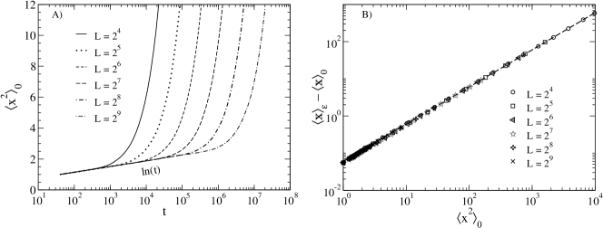
Figure 5: Panel A: linear-log plot of MSD, $\langle x_{t}^{2}\rangle_{0}$ vs. time for plaquette-comb lattice at different $L$, (Fig. 4A). Data show an initial collapse onto the common baseline $\ln(t)$, in perfect agreement with the scaling result (18). Panel B: plot of the response $\langle\delta x_{t}\rangle_{\epsilon}$ vs. the fluctuations $\langle(x_{t}-x_{0})^{2}\rangle_{0}$ showing the generalized Einstein’s relation (19). The slope of the dashed line is $3\epsilon$, with $\epsilon=2\delta p$ and $\delta p=0.01$ (unbalance in the left-right jump probability along the backbone).

To show the effect of $d_{S}$ on the homogenization time and on the diffusion process, we consider a structure composed by two-nested comb lattices that we dub “antenna” (Fig. 4B), i.e. a comb lattice, where the teeth are comb lattices themselves on the $y,z$ plane. This structure is then characterized by two length-scales, the vertical, $L_{y}$, and transversal, $L_{z}$, teeth length; only for sake of simplicity we assume $L_{y}\sim L_{z}\sim L$.

Also in this case there exists a crossover time $t_{*}(L)\sim L^{2}$ depending on the length of the teeth along-$z$, such that: for $t\gtrsim t_{*}(L)$, the diffusion becomes standard, whereas for $t\lesssim t_{*}(L)$, an anomalous diffusive regime takes place. Since for a simple comb lattice, $d_{S}=3/2$, see Weiss_Comb , we obtain from Eq. (4)

$$\langle(x_{t}-x_{0})^{2}\rangle_{0}\sim t^{1/4}\;.$$

For finite $L$, the MSD in Fig. 6A exhibits an initial regime $t^{1/4}$ followed by a $t^{1/2}$-behaviour with a final crossover to the standard one. Such a particular scaling, $t^{1/4}$, is certainly due to the ”double structure” of the sidebranches.

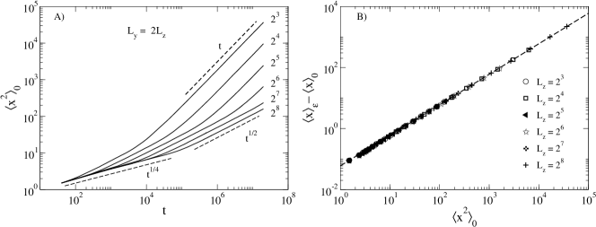
Figure 6: A-panel: time behaviour of MSD, $\langle x_{t}^{2}\rangle_{0}$ for the “antenna” (Fig. 4B) with $L_{y}=2L_{z}=L$ at different values of $L$. B-panel: generalized fluctuation-dissipation relation (19): response $\langle\delta x_{t}\rangle_{\epsilon}$ vs. $\langle x_{t}^{2}\rangle_{0}$. The slope of the dashed straight-line is the proportionality factor $3\epsilon$.

Also in this case, the generalized Einstein’s relation is verified (Fig. 6A) which coincides with Eq. (19) for the “kebab”. Indeed, the walkers on both antenna and kebab lattices have the same probability $1/6$ to make a jump to a nearest neighbour site along the backbone.

The case of $d_{S}>2$ must be carefully considered. For simplicity we present our analysis for the particular condition $d_{S}=d=3$, so we consider a comb-like structure where the lateral teeth are compenetrating but non-communicating cubes. For computational simplicity the cubes are arranged with centers at a unitary distance from one another along the backbone. Actually, the minimal distance among the centers of non-compenetrating cubes with edge $L$, is $L/2+L/2=L$ which is of course larger than $1$ as soon as $L>1$, but in our model the cubes, despite their large overlap, are still considered as distinct sidebranches connected only through the backbone. The homogenization time will be $t_{*}(L)\sim L^{d}$ and $D(L)\sim L^{-d}$. Therefore, for $t\gg t_{*}(L)$, we expect the standard diffusive growth $\langle(x-x_{0})^{2}\rangle_{0}\sim t/L^{d}$, while below $t_{*}(L)$, $\langle(x-x_{0})^{2}\rangle_{0}\sim t^{2\nu}$ and the matching condition at $t_{*}(L)$ predicts the existence of a plateau $\langle(x_{t}-x_{0})^{2}\rangle_{0}\sim\mbox{const}$, as derived by exact relations based on return probabilities Burioni05 . The simulation data are in agreement with the above results, see Fig. 7, and also the proportionality between fluctuation and response is again perfectly verified.

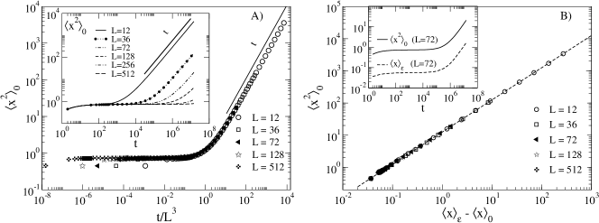
Figure 7: Comb lattice of compenetrating cubes. A) collapse of the MSD $\langle x_{t}^{2}\rangle_{0}$ at different cube sides $L$ vs. the rescaled time $t/L^{3}$. The data show the plateau which is a precursor of the standard diffusion. Inset: same data not rescaled. B) Plot showing the generalized fluctuation-dissipation relation: response $\langle\delta x_{t}\rangle_{\epsilon}$ vs. $\langle x_{t}^{2}\rangle_{0}$. Inset: plots of $\langle\delta x_{t}\rangle_{\epsilon}$ and $\langle x_{t}^{2}\rangle_{0}$ showing the parallel behaviour of response and MSD independently of the regime.

IV Conclusion

In this paper we have analyzed the random walk (RW) and the Einstein’s response-fluctuation relation on a class of branched lattices generalizing the standard comb-lattice. For any sidebranch of finite-size, a transient regime of anomalous diffusion is observed whose exponents can be derived by an heuristic argument based on the notion of homogenitazion time and on the geometrical properties of the lateral structures.

Our analysis has been here restricted to branched lattices where the distance between two consecutive sidebranches is unitary, but it can be straightforwardly extended to cases with arbitrary spacing.

We can conclude by noting that a random walk on generic branched lattice satisfies a generalized Einstein’s relation for different shapes and sizes $L$ of the sidebranches. This is clearly apparent in figures: 5B, 6B and 7B, where data perfectly collapse onto a straight line when plotting the free mean square displacements against the response.

Since this is a straightforward consequence of Eqs. (8) and (13), including their analogues in more complex comb-structures, the result that

$$R(t)=\frac{\langle(x_{t}-x_{0})^{2}\rangle_{0}}{\langle\delta x_{t}\rangle_{\epsilon}}=\mbox{const}$$

is exact and valid for any comb-like structure both in the transient and asymptotic regimes. It stems from the perfect compensation, at any time, between the response of the biased RW and the mean square displacement of the unbiased RW.

Our results may add other elements to the general issue Debate_Bio ; Klages_Book ; Ciliberto_FDR about the validity of the fluctuation-dissipation relations (FDR) in far from equilibrium systems and non Gaussian transport regimes.

There are by now sufficient theoretical Barkai98 ; Villamaina011 ; Chinappi and experimental GranuFDR ; NGauss_FDR evidences to claim that FDR can be often generalized well beyond its realm of applicability. This traditional issue of Statistical Mechanics received a renewed interest also thanks to the amazing progresses in single-molecule manipulation techniques. Experiments whereby a colloidal particle is dragged by optical tweezers well approximate the ideal system of a single Brownian particle driven out of equilibrium. This offers the opportunity to test in a laboratory the FDR on a minimal non equilibrium system. To some extent, invoking the similarity between RW and Brownian motion, the issues addressed in this work involve that class of behaviours encountered in mesoscopic systems MolMot , where either particles or generic degrees of freedom move diffusively on a complex support.

References

- (1) A. Einstein, On the movement of small particles suspended in a stationary liquid demanded by the molecular-kinetic theory of heat, Ann. d. Phys. 17 (1905) 549.
- (2) R. Kubo, The fluctuation-dissipation theorem, Rep. Prog. Phys. 29 (1966) 255.
- (3) U. M. B. Marconi, A. Puglisi, L. Rondoni, A. Vulpiani, Fluctuation–dissipation: Response theory in statistical physics, Phys. Rep. 461 (2008) 111.
- (4) J. Bouchaud, A. Georges, Anomalous diffusion in disordered media: statistical mechanisms, models and physical applications, Phys. Rep. 195 (1990) 127.
- (5) P. Castiglione, A. Mazzino, P. Muratore-Ginanneschi, A. Vulpiani, On strong anomalous diffusion, Physica D 134 (1999) 75.
- (6) J. Klafter, I. Sokolov, First Steps in Random Walks, Oxford: Oxford University Press, 2011.
- (7) T. Geisel, S. Thomae, Anomalous diffusion in intermittent chaotic systems, Phys. Rev. Lett. 52 (1984) 1936.
- (8) R. Klages, G. Radons, I. M. Sokolov, Anomalous transport, Wiley-VCH, 2008.
- (9) W. Schirmacher, M. Prem, J.-B. Suck, A. Heidemann, Anomalous diffusion of hydrogen in amorphous metals, Europhys. Lett. 13 (1990) 523.
- (10) B. Berkowitz, H. Scher, S. E. Silliman, Anomalous transport in laboratory-scale, heterogeneous porous media, Water Resources Research 36 (2000) 149–158.
- (11) D. L. Koch, J. F. Brady, Anomalous diffusion in heterogeneous porous media, Physics of Fluids 31 (1988) 965.
- (12) M. Köpf, C. Corinth, O. Haferkamp, T. Nonnenmacher, Anomalous diffusion of water in biological tissues, Biophys. J. 70 (1996) 2950.
- (13) J. Hrabe, S. Hrabĕtová, K. Segeth, A model of effective diffusion and tortuosity in the extracellular space of the brain, Biophys. J. 87 (2004) 1606–1617.
- (14) M. Weiss, E. Markus, K. Fredrik, N. Tommy, Anomalous subdiffusion is a measure for cytoplasmic crowding in living cells, Biophys. J. 87 (2004) 3518.
- (15) A. Caspi, R. Granek, M. Elbaum, Diffusion and directed motion in cellular transport, Phys. Rev. E 66 (2002) 011916–(12).
- (16) D. ben Avraham, S. Havlin, Diffusion and Reactions in Fractals and Disordered Systems, Cambridge University Press, Cambridge, 2000.
- (17) G. H. Weiss, S. Havlin, Some properties of a random walk on a comb structure, Physica A 134 (1986) 474.
- (18) G. H. Weiss, S. Havlin, Use of comb-like models to mimic anomalous diffusion on fractal structures, Philos. Mag. B 56 (1987) 941–947.
- (19) R. Burioni, D. Cassi, Random walks on graphs: ideas, techniques and results, J. Phys. A: Math. Gen. 38 (2005) R45.
- (20) A. Coniglio, Thermal phrase transition of the dilute s-state potts and n-vector models at the percolation threshold, Phys. Rev. Lett. 46 (1981) 250.
- (21) A. Coniglio, Cluster structure near the percolation threshold, J. Phys. A: Math. Gen. 15 (1982) 3829.
- (22) E. F. Casassa, G. C. Berry, Angular distribution of intensity of rayleigh scattering from comblike branched molecules, J. Polym. Sci. A-2 Polym. Phys. 4 (1966) 881–897.
- (23) J. F. Douglas, J. Roovers, K. F. Freed, Characterization of branching architecture through” universal” ratios of polymer solution properties, Macromolecules 23 (1990) 4168–4180.
- (24) H. Stanley, A. Coniglio, Flow in porous media: The backbone fractal at the percolation threshold, Phys. Rev. Lett. 29 (1984) 522.
- (25) S. Tarafdar, A. Franz, C. Schulzky, K. H. Hoffmann, Modelling porous structures by repeated sierpinski carpets, Phys. A: Statistical Mechanics and its Applications 292 (2001) 1–8.
- (26) D. Villamaina, A. Sarracino, G. Gradenigo, A. Puglisi, A. Vulpiani, On anomalous diffusion and the out of equilibrium response function in one-dimensional models, J. Stat. Mech. Theor. Exp. 2011 (2011) L01002.
- (27) E. Barkai, V. Fleurov, Generalized einstein relation: A stochastic modeling approach, Phys. Rev. E 58 (1998) 1296.
- (28) R. Metzler, J. Klafter, The random walk’s guide to anomalous diffusion: a fractional dynamics approach, Phys. Rep. 339 (2000) 1.
- (29) A. V. Chechkin, F. Lenz, R. Klages, Normal and anomalous fluctuation relations for gaussian stochastic dynamics, J. Stat. Mech. Theor. Exp. 2012 (2012) L11001.
- (30) I. Goldhirsch, Y. Gefen, Analytic method for calculating properties of random walks on networks, Phys. Rev. A 33 (1986) 2583.
- (31) G. H. Weiss, Aspects and Applications of the Random Walk, North-Holland, Amsterdam, 1994.
- (32) A. Koponen, M. Kataja, J. Timonen, Tortuous flow in porous media, Phys. Rev. E 54 (1996) 406–410.
- (33) S. Redner, A guide to first-passage processes, Cambridge University Press, 2001.
- (34) E. W. Montroll, G. H. Weiss, Random walks on lattices. ii, J. Math. Phys. 6 (1965) 167.
- (35) M. F. Shlesinger, Asymptotic solutions of continuous-time random walks, J. Stat. Phys. 10 (1974) 421–434.
- (36) R. Burioni, D. Cassi, G. Giusiano, S. Regina, Anomalous diffusion and hall effect on comb lattices, Phys. Rev. E 67 (2003) 016116.
- (37) S. Alexander, R. Orbach, Density of states on fractals: fractons, J. Phys. Lett-Paris 43 (1982) 625.
- (38) D. Cassi, S. Regina, Random walks on kebab lattices:. logarithmic diffusion on ordered structures, Mod. Phys. Lett. B 9 (1995) 601.
- (39) C. Haynes, A. Roberts, Continuum diffusion on networks: Trees with hyperbranched trunks and fractal branches, Phys. Rev. E 79 (2009) 031111.
- (40) R. Burioni, D. Cassi, Geometrical universality in vibrational dynamics, Mod. Phys. Lett. B 11 (1997) 1095.
- (41) A. W. C. Lau, B. D. Hoffman, A. Davies, J. C. Crocker, T. C. Lubensky, Microrheology, stress fluctuations, and active behavior of living cells, Phys. Rev. Lett. 91 (2003) 198101.
- (42) H. G. Schuster, R. Klages, W. Just, C. Jarzynski, Nonequilibrium Statistical Physics of Small Systems: Fluctuation Relations and Beyond, Wiley-VCH, 2013.
- (43) S. Ciliberto, R. Gomez-Solano, A. Petrosyan, Fluctuations, linear response, and currents in out-of-equilibrium systems, Annu. Rev. of Cond. Matt. Phys. 4 (2013) 235–261.
- (44) M. Chinappi, E. De Angelis, S. Melchionna, C. Casciola, S. Succi, R. Piva, Molecular dynamics simulation of ratchet motion in an asymmetric nanochannel, Phys. Rev. Lett. 97 (2006) 144509.
- (45) G. D’Anna, P. Mayor, A. Barrat, V. Loreto, F. Nori, Observing brownian motion in vibration-fluidized granular matter, Nature 424 (2003) 909–912.
- (46) Q. Gu, E. Schiff, S. Grebner, F. Wang, R. Schwarz, Non-gaussian transport measurements and the einstein relation in amorphous silicon, Phys. Rev. Lett. 76 (1996) 3196–3199.
- (47) L. Le Goff, F. Amblard, E. M. Furst, Motor-driven dynamics in actin-myosin networks, Phys. Rev. Lett. 88 (2001) 018101.