Model-independent constraints on the cosmological anisotropic stress

Abstract

The effective anisotropic stress or gravitational slip $\eta=-\Phi/\Psi$ is a key variable in the characterisation of the physical origin of the dark energy, as it allows to test for a non-minimal coupling of the dark sector to gravity in the Jordan frame. It is however important to use a fully model-independent approach when measuring $\eta$ to avoid introducing a theoretical bias into the results. In this paper we forecast the precision with which future large surveys can determine $\eta$ in a way that only relies on directly observable quantities. In particular, we do not assume anything concerning the initial spectrum of perturbations, nor on its evolution outside the observed redshift range, nor on the galaxy bias. We first leave $\eta$ free to vary in space and time and then we model it as suggested in Horndeski models of dark energy. Among our results, we find that a future large scale lensing and clustering survey can constrain $\eta$ to within 10% if $k$-independent, and to within 60% or better at $k=0.1h/$Mpc if it is restricted to follow the Horndeski model.

I Introduction

With the recent first results of the Planck satellite Ade:2013ktc we have definitely reached the era of precision cosmology: The Planck observations of the cosmic microwave background (CMB) are well described by the six-parameter flat $\Lambda$CDM model, and most of those six parameters are determined to percent-level accuracy Ade:2013zuv . The most impressive achievement is the measurement of the acoustic scale of the CMB with a precision of 0.06% by Planck, but also the physical baryon and the matter densities have been determined to within an uncertainty of only 1 to 2%.

But the conclusion from these measurements is that we live in an Universe where only 5% of today’s energy density consists of the kind of matter described by the standard model of particle physics. Another 27% appears to be matter that is only interacting gravitationally with the visible world, and the remaining 68% is made up of a cosmological constant.

The physical nature of the dark sector is however completely unknown, and especially the cosmological constant suffers from severe theoretical problems. For this reason it is of crucial importance to look beyond the perfectly homogeneous cosmological constant and to investigate general dark energy models, including also modifications of Einstein’s theory of General Relativity (GR). When considering a general dark energy model however, high precision is much harder to achieve, and it is important to understand first what can actually be observed, to avoid introducing a theoretical bias into the observational results. Coming from this angle, we determined in a recent paper Amendola:2012ky that cosmological measurements at linear scales can determine, in addition to the expansion rate $H(z)$, only three additional variables $R$, $A$ and $L$, given by

$$A =Gb\delta_{\text{m,0}}\,,\qquad R=Gf\delta_{\text{m,0}}\,,$$ (1)

$$L =\Omega_{\text{m,0}}GY(1+\eta)\delta_{\text{m,0}}\,.$$

Denoting with $k$ the norm of the wavenumber and with $a$ the cosmic scale factor, we refer with $G(k,a)$ to the linear growth function (normalized to unity today) with $f=G^{\prime}/G$ to the growth rate, with $b(k,a)$ to the galaxy bias with respect to the dark matter density contrast and with $\delta_{\text{m,0}}(k)$ to the dark matter density contrast today. The functions $\eta(k,a)$ and $Y(k,a)$ describe the impact of the dark energy on the cosmological perturbations. Later on, we will also need the quantities $\bar{A}\equiv A/\delta_{\text{t,0}}$, $\bar{R}\equiv R/\delta_{\text{t,0}}$, $\bar{L}\equiv L/\delta_{\text{t,0}}$ with $\delta_{\text{t,0}}=\delta_{\text{m,0}}/\sigma_{8}$. If we write the line element describing the perturbed Friedmann-Lemaître-Robertson-Walker metric as

$$ds^{2}=-(1+2\Psi){\mathrm{d}t}^{2}+a(t)^{2}\left(1+2\Phi\right){\mathrm{d}{\mathbf{x}}}^{2},$$ (2)

then $\eta$ and $Y$ are defined through Amendola:2007rr ; DeFelice:2011hq

$$\eta(k,a)\equiv-\frac{\Phi}{\Psi}\,,\qquad Y(k,a)\equiv-\frac{2k^{2}\Psi}{3\Omega_{\text{m}}\delta_{\text{m}}}\,.$$ (3)

We see that $\eta$ corresponds to the gravitational slip, which is linked to the effective anisotropic stress of the dark energy, and $Y$ describes the clustering of the dark energy. The function $\eta$ is particularly important, as it is a key-variable to distinguish scalar-field type dark energy models from modifications of GR Saltas:2010tt ; Sawicki:2012re .

So far these are rather abstract considerations. An obviously important question is whether we can actually measure these quantities with realistic surveys, and to what precision. In Amendola:2012ky ; Motta:2013cwa we showed that we can use the motion of light and of non-relativistic test-particles like galaxies to map out the metric functions $\Phi$ and $\Psi$ in principle, and that therefore $\eta$ is an observable quantity. But $Y$ depends on the dark matter distribution, which is not directly observable, and so also $Y$ itself is in general not directly observable due to the dark degeneracy Kunz:2007rk .

In order to reconstruct $\eta$ from $A$, $R$ and $L$ it is necessary to remove the dependence on $\delta_{\text{t},0}$ (notice that $\bar{A}$, $\bar{R}$ and $\bar{L}$ are not observables), since it is an unknown quantity that does not depend on dark energy physics but rather on inflation or other primordial effects. This can be done by considering ratios like $P_{1}=R/A$, $P_{2}=L/R$ and $P_{3}=R^{\prime}/R$. In terms of these model-independent ratios, the gravitational slip becomes Amendola:2012ky ; Motta:2013cwa

$$1+\eta=\frac{3P_{2}(1+z)^{3}}{2E^{2}\left(P_{3}+2+\frac{E^{\prime}}{E}\right)}$$ (4)

where we also set $E(z)\equiv H(z)/H_{0}$.

When constraining $\eta$ later on, we will use an equivalent quantity which we call $\bar{\eta}$, defined as

$$\bar{\eta}\equiv\frac{2}{1+\eta}=\frac{2\Psi}{\Psi-\Phi}\,.$$ (5)

The reason is that even for large future surveys the expected error on $P_{3}$ is substantial, especially when we want to allow for an unknown redshift and scale dependence. The large error makes the division by $(P_{3}+2+E^{\prime}/E)$ in Eq. (4) badly behaved. $\bar{\eta}$ on the other hand is more stable, as we discuss in more detail in appendix A.

Based on these results, we will use the Fisher matrix formalism in this paper to forecast the expected precision on $\bar{A}$, $\bar{R}$ and $\bar{L}$, which are then projected onto the accuracy with which we can obtain $P_{1}$, $P_{2}$ and $P_{3}$, and finally on $\bar{\eta}$, based on the expected performance of future large-scale galaxy and weak lensing surveys. We will also include a supernova survey to improve the constraints on the background expansion rate $E(z)$, although we find that its impact on the final constraints on $\eta$ is rather modest. In the final step we will assume four models for $\eta$:

1. First, we assume that $\eta$ is constant at all scales and at all redshifts (let us call this case the constant-$\eta$ case). This occurs for instance in $\Lambda$CDM and in all models in which dark energy does not cluster and is decoupled from gravity.

2. Second, we assume that $\eta$ is constant in space but varies in redshift ($z$-varying case). In other words, we assume that $\eta$ has a different arbitrary value for each redshift bin.

3. Third, we assume $\eta$ varies in both redshift and space ($z,k$-varying case).

4. Fourth, we take for $\eta$ the quasi-static Horndeski result Amendola:2012ky

   $$\eta=h_{2}\left(\frac{1+k^{2}h_{4}}{1+k^{2}h_{5}}\right).$$ (6)

   (Here we assume $k$ to be measured in units of 0.1 $h/$Mpc, so the $h_{i}$ functions are dimensionless). We denote this model as the Horndeski case. The Horndeski Lagrangian is the most general Lagrangian for a single scalar field leading to second-order equations of motion. The expression (6) arises in the quasi-static limit DeFelice:2011hq where the time-derivative terms are sub-dominant, which implies that the scales of interest are inside the (sound-) horizon.

In all cases the fiducial model will be chosen to be $\Lambda$CDM, for which $\eta=\bar{\eta}=1$. For the first two cases we need only a binning in redshift, while for the third and fourth case we will bin both in redshift and in $k$-space. The fiducial values in the first Horndeski case are $h_{2}=1$, $h_{4}=h_{5}=0$.

The outline of the paper is as follows: In sections III, IV and V we set up the Fisher matrix formalism for the galaxy clustering, weak lensing, and SN-Ia observations. As already mentioned above, we will see that we need to combine the different probes to obtain constraints on $\eta$, and we discuss the combination of the Fisher matrices in Sec. VI before concluding in the final section.

II Notation and general definitions

In this section we complete the definition of our notation and provide definitions for quantities that are useful in several of the following sections. Our metric signature and the gravitational potentials are already defined in Eq. (2). In Eq. (3) we define the functions $\eta$ and $Y$ that parameterize the ‘dark energy perturbations’ (as the dark matter does not contribute to the anisotropic stress). The function $\eta$ assumes a central stage in this paper as it is observable without requiring further assumptions, see Eq. (4).

Although the observables $E$, $A$, $R$ and $L$ can be measured in a fully model-independent way, the precision with which we can determine them depends also on the true nature of the Universe. When evaluating our forecasts, we will use a flat $\Lambda$CDM fiducial model, characterized by the WMAP 7-year values, $\Omega_{\text{m},0}h^{2}=0.134$, $\Omega_{b,0}h^{2}=0.022$, $n_{s}=0.96$, $\tau=0.085$, $h=0.694$ and $\Omega_{k}=0$. The new WMAP 9-year and Planck results are not very different so the results are not significantly affected by our choice. The dimensionless background expansion rate in the fiducial model and at low redshifts is given by

$$E(z)^{2}=\Omega_{\text{m},0}(1+z)^{3}+(1-\Omega_{\text{m},0})\,,$$ (7)

and we will often use the dimensionless angular diameter distance $\hat{d}_{A}(z)=\hat{r}(z)/(1+z)$ and the dimensionless luminosity distance $\hat{d}_{L}(z)=\hat{r}(z)(1+z)$, where in a flat FLRW Universe

$$\hat{r}(z)=\int_{0}^{z}\frac{{\mathrm{d}\tilde{z}}}{E(\tilde{z})}\,.$$ (8)

The usual distances are related to the dimensionless distances through $\hat{r}=H_{0}r$ and $\hat{d}=H_{0}d$. In $\Lambda$CDM we have that $\eta=1$ and $Y=1$. In the fiducial model, both $G$ and $f$ only depend on the scale factor, not on $k$.

We will combine in the following the Fisher matrices for future galaxy clustering, weak lensing and supernovae surveys. More specifically, we will take for galaxy clustering (GC) and weak lensing (WL) a stage IV kind of survey Albrecht:2006um like Euclid 2011arXiv1110.3193L . Notice that the survey specifications we use in this paper are meant only to be representative of a future dark energy survey and do not necessarily reflect the actual Euclid configuration. For supernovae (SN) we assume a survey of $10^{5}$ sources with magnitude errors similar to the currently achievable uncertainties, as expected in the LSST survey Tyson:2003kb .

III Galaxy clustering

The galaxy power spectrum can be written as Seo:2003

$$P(k,\mu)=(A+R\mu^{2})^{2}e^{-k^{2}\mu^{2}\sigma_{r}^{2}}=(\bar{A}+\bar{R}\mu^{2})^{2}\delta_{\text{t,0}}^{2}(k)e^{-k^{2}\mu^{2}\sigma_{r}^{2}},$$ (9)

where $\sigma_{r}=\delta z/H(z)$, $\delta z$ being the absolute error on redshift measurement, and we explicitly use $\delta_{\text{m,0}}=\sigma_{8}\delta_{\text{t,0}}$, and where $\mu$ is the cosine of the angle between the line of sight and the wavevector. Notice that $\bar{R}$ is often denoted in the literature as $f\sigma_{8}(z)$.

As already emphasized, we will ignore in the following the information contained in $\delta_{\text{t,0}}^{2}(k)$ since this depends on initial conditions that are in general not known, and we cannot disentangle the initial conditions from the information on the dark energy (we refer to Amendola:2012ky for a discussion about this point). Removing the information from the shape of the power spectrum of course reduces the amount of information available and so increases the error bars. This is the price to pay if we want to stay fully model independent.

The dependence on $E$ is implicitly contained in $\mu$ and $k$ through the Alcock-Paczyński effect Alcock:1979 . However, we can only take into account the $\mu$ dependence, since the $k$ dependence occurs through the unknown function $\delta_{\text{m,0}}$. The Fisher matrix for the parameter vector $p_{\alpha}$ is in general Seo:2003

$$F_{\alpha\beta}^{\text{GC}}=\frac{1}{8\pi^{2}}\int_{-1}^{1}{\mathrm{d}\mu}\int_{k_{\text{min}}}^{k_{\text{max}}}k^{2}V_{\text{eff}}D_{\alpha}D_{\beta}\,{\mathrm{d}k}\,,$$ (10)

where

$$D_{\alpha}\equiv\frac{d\log P}{dp_{\alpha}}\biggl{|}_{r}$$ (11)

is the parameter derivative evaluated on the fiducial values (designated by the subscript ‘$r$’) and where

$$V_{\text{eff}}=\left(\frac{\bar{n}P(k,\mu)}{\bar{n}P(k,\mu)+1}\right)^{2}V_{\text{survey}}$$ (12)

is the effective volume of the survey, with $\bar{n}$ the galaxy number density in each bin (discussed later). The Fisher matrix is evaluated at the fiducial model. For this evaluation we will assume that the bias in $\Lambda$CDM is scale independent and equal to unity, which implies that the barred variables $\bar{A}$ and $\bar{R}$ also do not depend on $k$ in the fiducial model (although of course in general they will be scale dependent).

Our parameters are therefore $p_{\alpha}^{\text{\tiny{GC}}}=\{\bar{A}(\bar{z}_{1}),\bar{R}(\bar{z}_{1}),E(\bar{z}_{1}),\bar{A}(\bar{z}_{2}),\bar{R}(\bar{z}_{2}),E(\bar{z}_{2}),\dots\}$, where the subscripts run over the $z$ bins. We could have used $A,R$ directly as parameters as in Eq. (9), but we prefer to clearly distinguish between the dark energy dependent parameters $\bar{A},\bar{R}$ and those that depend on different physics. Indices $\alpha$ or $\beta$ always label the parameters in the Fisher matrix framework. From the definition of the galaxy clustering power spectrum, Eq. (9), (and without taking into account the correction from the error on redshift, as we will assume a spectroscopic survey with negligible redshift errors) we find that

$$D_{\bar{A}}=\frac{2}{\bar{A}+\bar{R}\mu^{2}}\,,\quad D_{\bar{R}}=\frac{2\mu^{2}}{\bar{A}+\bar{R}\mu^{2}}\,,$$ (13)

and using (Amendola2010, , p. 393)

$$\mu=\frac{H\mu_{r}}{H_{r}Q},$$ (14)

where

$$Q=\frac{\sqrt{E^{2}\hat{d}_{A}^{2}\mu_{r}^{2}-E_{r}^{2}\hat{d}_{Ar}^{2}(\mu_{r}^{2}-1)}}{E_{r}\hat{d}_{A}},$$ (15)

we get for the derivative with respect to the parameter $E$

$$D_{E}=\frac{4\bar{R}\mu^{2}(1-\mu^{2})}{(\bar{A}+\bar{R}\mu^{2})}\left(\frac{1}{E_{r}}+\frac{1}{\hat{d}_{Ar}}\frac{\partial\,\hat{d}_{A}}{\partial E}\right).$$ (16)

Here we explicitly consider the dependence of the dimensionless angular diameter distance $\hat{d}_{A}$ on $E$ via Eq. (8).

III.1 $z$ binning

We consider an Euclid-like survey 2011arXiv1110.3193L from $z=0.5-1.5$ divided in equally spaced bins of width $\Delta z=0.2$, and, in order to prevent accidental degeneracies due to low statistics, a single larger redshift bin between $z=1.5-2.1$ (thus the number of bins is $n_{B}=6$). The lower boundaries of the $z$-bins are labeled as $z_{a}$ while the center of the bins are labeled as $\bar{z}_{a}$ (latin indices $a,b,\ldots$ label the $z$-bins). The galaxy number densities in each bin are shown in Table 2; for the bin between $1.5$ and $2.1$ we use an average number of $0.33\times 10^{-3}$ ($h/$Mpc)³ Amendola:2012ys . The error on the measured redshift is assumed to be spectroscopic: $\delta z=0.001(1+z)$. The transfer function in the present matter power spectrum ($\delta_{\text{t,0}}^{2}$) is calculated using CAMB Lewis:2000 for the $\Lambda$CDM cosmology defined in Sec. II. The limits on the integration over $k$ are taken as $k_{\text{min}}=0.007$ $h/$Mpc (but the results are very weakly dependent on this value) and the values of $k_{\text{max}}$ are chosen to be well below the scale of non-linearity at the redshift of the bin, see Table 1.

$\bar{z}$	$k_{\text{min}}$	$k_{1}$	$k_{2}$	$k_{\text{max}}$
0.6	0.007	0.022	0.063	0.180
0.8	0.007	0.023	0.071	0.215
1.0	0.007	0.024	0.078	0.249
1.2	0.007	0.026	0.086	0.287
1.4	0.007	0.027	0.094	0.329
1.8	0.007	0.029	0.112	0.426

Table 1: Values of $k_{1}$, $k_{2}$ and $k_{\text{max}}$ for every redshift bin, in units of ($h/$Mpc).

Since the angular diameter distance can be approximated by the expression

$$\hat{d}_{A}(\bar{z}_{a})=\frac{1}{(1+\bar{z}_{a})}\sum_{b=0}^{b=a}\frac{\Delta z_{b}}{E(\bar{z}_{b})},$$ (17)

we have for the term $\frac{\partial\,\hat{d}_{A}}{\partial E}$ in equation (16)

$$\frac{\partial\hat{d}_{A}(\bar{z}_{a})}{\partial E(\bar{z}_{b})}=-\frac{\Delta z_{b}}{(1+\bar{z}_{a})E_{b}^{2}}\delta_{ab},$$ (18)

where $\delta_{ab}$ is a Kronecker delta symbol. Then we calculate the Fisher matrix block-wise with independent submatrices $F_{\alpha\beta}^{\text{GC}}$ for each bin.

The errors in the set of parameters $p_{\alpha}^{\text{\tiny{GC}}}$ are taken from the square root of the diagonal elements of the inverted Fisher matrix, i.e. the errors are marginalized over all other parameters. In Table 2 we present the fiducial values for $\bar{A}$, $\bar{R}$ and $E$ evaluated at the center of the bins ($\bar{z}_{a}$), and the respective errors, and in Fig. 1 we plot their fiducial values and errors.

$\bar{z}$	$\bar{n}(\bar{z})\times 10^{-3}$	$\bar{A}$	$\Delta\bar{A}$	$\Delta\bar{A}(\%)$	$\bar{R}$	$\Delta\bar{R}$	$\Delta\bar{R}(\%)$	$E$	$\Delta E$	$\Delta E(\%)$
0.6	3.56	0.612	0.0022	0.37	0.469	0.0092	2.0	1.37	0.12	8.5
0.8	2.42	0.558	0.0017	0.3	0.457	0.0068	1.5	1.53	0.073	4.8
1.0	1.81	0.511	0.0015	0.29	0.438	0.0056	1.3	1.72	0.058	3.4
1.2	1.44	0.47	0.0014	0.29	0.417	0.0049	1.2	1.92	0.05	2.6
1.4	0.99	0.434	0.0015	0.35	0.396	0.0047	1.2	2.14	0.051	2.4
1.8	0.33	0.377	0.0018	0.47	0.354	0.0039	1.1	2.62	0.061	2.3

Table 2: Fiducial values and errors for $\bar{A}$, $\bar{R}$ and $E$ using six redshift bins. Units of galaxy number densities are ($h/$Mpc)³.

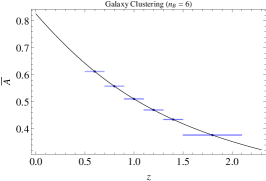
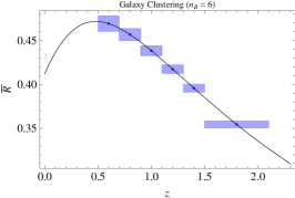
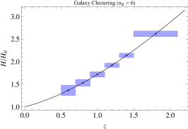
Figure 1: Errors on $\bar{A}$, $\bar{R}$ and $E$ from Galaxy Clustering in the $z$-binning case.

If we use a redshift dependent bias $b(z)$ (for instance taking the values from the Euclid specifications, see 2011arXiv1110.3193L ; Orsi:2009mj ), we get only slight deviations from the errors found for the previous case, as we can see in Table 3. Thus, our choice of a bias equal to unity does not impact the Fisher errors significantly.

$\bar{z}$	$\bar{A}$	$\Delta\bar{A}$	$\Delta\bar{A}(\%)$	$\bar{R}$	$\Delta\bar{R}$	$\Delta\bar{R}(\%)$	$E$	$\Delta E$	$\Delta E(\%)$
0.6	0.645	0.0023	0.36	0.469	0.0094	2.	1.37	0.12	8.8
0.8	0.628	0.0018	0.28	0.457	0.0072	1.6	1.53	0.078	5.1
1.0	0.575	0.0015	0.26	0.438	0.0059	1.3	1.72	0.06	3.5
1.2	0.584	0.0014	0.24	0.417	0.0052	1.2	1.92	0.053	2.7
1.4	0.561	0.0015	0.27	0.396	0.005	1.3	2.14	0.053	2.5
1.8	0.561	0.0015	0.26	0.354	0.0038	1.1	2.62	0.056	2.1

Table 3: Fiducial values and errors for $\bar{A}$, $\bar{R}$ and $E$ using six bins, considering a redshift dependent bias.

III.2 $k$ binning

For the third and fourth model we also need a binning in $k$-space. Since ultimately we would like to obtain error estimates on three functions, $h_{2},h_{4},h_{5}$, we will need a minimum of three $k$-bins, which is the choice we make here. We denote with latin indexes $a,b,c...$ the $z$ bins and with indexes $i,j,k...$ the $k$ bins. So for the first $z$-bin we have as parameters $s_{1}=\{\bar{A}_{11},\bar{R}_{12},E_{1}\}$, for the second $s_{2}=\{\bar{A}_{21},\bar{R}_{22},E_{2}\}$, and so forth, with $\bar{A}_{ai}=\bar{A}(\bar{z}_{a},\bar{k}_{i})$, $\bar{R}_{ai}=\bar{R}(\bar{z}_{a},\bar{k}_{i})$, and $E_{a}=E(\bar{z}_{a})$, where $\bar{k}_{i}$ denote the centers of the $k$-bins. The set of parameters is therefore $p_{\alpha}^{\text{\tiny{GC}}}=\{s_{1},s_{2},...\}$. The Fisher matrix integration over $k$ is split into three $k$-ranges between $k_{\text{max}}$ and $k_{\text{min}}$ which we choose so that $\Delta\log k=\rm const$. The Fisher matrix becomes then

$$F_{\alpha\beta}^{\text{GC}}=\frac{1}{8\pi^{2}}\int_{-1}^{1}d\mu\int_{\Delta k}k^{2}V_{\text{eff}}D_{\alpha}D_{\beta}\,{\mathrm{d}k}\,,$$ (19)

with $\Delta k$ denoting the respective range of the integration. Denoting the entry $F_{\bar{A}\bar{R}}$ as $\bar{A}\bar{R}$ , and so on, we can represent the structure of the matrix for every redshift bin as follows:

$$\left(\begin{array}[]{ccccccc}\bar{A}_{1}\bar{A}_{1}&\bar{A}_{1}\bar{R}_{1}&0&0&0&0&\bar{A}_{1}E\\ \bar{R}_{1}\bar{A}_{1}&\bar{R}_{1}\bar{R}_{1}&0&0&0&0&\bar{R}_{1}E\\ 0&0&\bar{A}_{2}\bar{A}_{2}&\bar{A}_{2}\bar{R}_{2}&0&0&\bar{A}_{2}E\\ 0&0&\bar{R}_{2}\bar{A}_{2}&\bar{R}_{2}\bar{R}_{2}&0&0&\bar{R}_{2}E\\ 0&0&0&0&\bar{A}_{3}\bar{A}_{3}&\bar{A}_{3}\bar{R}_{3}&\bar{A}_{3}E\\ 0&0&0&0&\bar{R}_{3}\bar{A}_{3}&\bar{R}_{3}\bar{R}_{3}&\bar{R}_{3}E\\ E\bar{A}_{1}&E\bar{R}_{1}&E\bar{A}_{2}&E\bar{R}_{2}&E\bar{A}_{3}&E\bar{R}_{3}&EE\end{array}\right),$$ (20)

In Table 1 we display the values for the integration limits at every redshift (the $k$-bins borders), and in Table 4 we present the errors for all $(z,k)$-bins. Notice that the errors on $E$ are not affected by the $k$-binning, as $E$ does not depend on $k$.

$\bar{z}$	$i$	$\bar{A}$	$\Delta\bar{A}$	$\Delta\bar{A}(\%)$	$\bar{R}$	$\Delta\bar{R}$	$\Delta\bar{R}(\%)$	$E$	$\Delta E$	$\Delta E(\%)$
0.6	1	0.612	0.025	4.	0.469	0.07	15.	1.37	0.11	8.4
	2		0.0058	0.94		0.017	3.6
	3		0.0023	0.38		0.0097	2.1
0.8	1	0.558	0.018	3.2	0.457	0.05	11	1.53	0.074	4.8
	2		0.0039	0.71		0.012	2.6
	3		0.0018	0.32		0.0074	1.6
1.0	1	0.511	0.014	2.7	0.438	0.039	8.9	1.72	0.058	3.4
	2		0.003	0.59		0.0089	2.
	3		0.0016	0.31		0.0062	1.4
1.2	1	0.47	0.011	2.4	0.417	0.032	7.7	1.92	0.051	2.6
	2		0.0025	0.54		0.0072	1.7
	3		0.0015	0.32		0.0055	1.3
1.4	1	0.434	0.01	2.3	0.396	0.028	7.	2.14	0.052	2.4
	1		0.0024	0.55		0.0065	1.6
	3		0.0018	0.41		0.0057	1.4
1.8	1	0.377	0.0063	1.7	0.354	0.015	4.3	2.62	0.059	2.3
	2		0.0022	0.58		0.0047	1.3
	3		0.0024	0.64		0.0061	1.7

Table 4: Relative errors for $\bar{A}$, $\bar{R}$ and $E$ at every redshift and every $k$-bin (labeled with the index $i$). Since fiducial values for $\bar{A}$, $\bar{R}$ and $E$ are independent of $k$, these are the same for the three $k$-bins.

IV Weak lensing

We move now to estimating the Fisher matrix for a future weak lensing survey. The lensing convergence power spectrum from a survey divided into several redshift bins (same binning as in Sec. III) can be written as Hu:1999ek

$$P_{ij}(\ell)=H_{0}\int_{0}^{\infty}p_{ij}(z,\ell){\mathrm{d}z}\approx H_{0}\sum_{a}\frac{\Delta z_{a}}{E_{a}}K_{i}K_{j}\bar{L}^{2}\delta_{\text{t},0}^{2}\left(\bar{z}_{a},k(\ell,\bar{z}_{a})\right)\,,$$ (21)

with the integrand

$$p_{ij}(z,\ell)=\frac{K_{i}(z)K_{j}(z)}{E(z)}\ \bar{L}(z)^{2}\delta_{\text{t},0}^{2}\left(z,k(\ell,z)\right),$$ (22)

where

$$k(\ell,z)=\frac{\ell}{\pi r(z)}\quad\mathrm{and}\quad K_{i}(z)=\frac{3}{2}(1+z)W_{i}(z)\,,$$ (23)

and $W_{i}(z)$ is the weak lensing window function for the $i$-th bin

$$W_{i}(z)=H_{0}\int_{z}^{\infty}\left(1-\frac{\hat{r}(z)}{\hat{r}(\tilde{z})}\right)n_{i}(\tilde{z})\,{\mathrm{d}\tilde{z}}\,.$$ (24)

Here, $n_{i}(z)$ equals the galaxy density $n(z)$ if $z$ lies inside the $i$-th redshift bin and zero otherwise. Note that

$$n_{i}(z){{\rm d}z=\frac{n_{i}(r(z))}{H(z)}{{\rm d}r}}\,.$$ (25)

The overall galaxy density is modeled as

$$n(z)\propto z^{a}\exp(-(z/z_{p})^{b}).$$ (26)

We take $a=2$, $b=3/2$ and choose $z_{p}$ such that the median of the distribution is at $z=0.9$, i.e. $z_{p}=0.9/1.412=0.6374$ Ma2006 ; 2011arXiv1110.3193L . The $n_{i}(z)$ (which are not to be confused with the $\bar{n}(z)$ from Galaxy Clustering) are then smoothed with a Gaussian to account for the photometric redshift error (see Ma2006 ) and normalized such that $\int n_{i}(z){{\rm d}z=1}$. Following the Euclid specifications, we set the survey sky fraction $f_{{\rm sky}}=0.375$ and the photometric redshift error to $\delta z=0.05(1+z)$.

Including the noise due to intrinsic galaxy ellipticities we have

$$C_{ij}=P_{ij}+\gamma_{{\rm int}}^{2}\hat{n}_{i}^{-1}\delta_{ij},$$ (27)

with the intrinsic ellipticity $\gamma_{{\rm int}}=0.22$ and the number of all galaxies per steradian in the $i$-th bin, $\hat{n}_{i}$, which can be written as

$$\hat{n}_{i}=n_{\theta}\frac{\int_{z_{i}}^{z_{i+1}}n(z)\mathrm{d}z}{\int_{0}^{\infty}n(z)\mathrm{d}z},$$ (28)

where $n_{\theta}$ is the areal galaxy density, an important parameter that defines the quality of a weak lensing experiment. We set it to $n_{\theta}=35$ galaxies per square arc minute 2011arXiv1110.3193L .

For a weak lensing survey that covers a fraction of the sky $f_{{\rm sky}}$, the Fisher matrix is a sum over $\ell$ bins of size $\Delta\ell$ (Eisenstein1999a, )

$$F_{\alpha\beta}^{\text{WL}}=f_{{\rm sky}}\sum_{\ell}\Delta\ell\frac{(2\ell+1)}{2}\frac{\partial P_{ij}}{\partial p_{\alpha}}C_{jm}^{-1}\frac{\partial P_{mn}}{\partial p_{\beta}}C_{ni}^{-1},$$ (29)

and now the parameters are $p_{\alpha}=\{\bar{L}(\bar{z}_{1}),E(\bar{z}_{1}),\dots\}$. Here, $\ell$ is being summed from 5 to $\ell_{\rm max}$ with $\Delta\log\ell=0.1$, where $\ell_{\rm max}$ corresponds to the value listed in Table IV for the redshift bin $a$ or $b$ — whichever is smaller.

The value $\ell_{\rm max}$ is derived as follows. We start with the relationship

$$\frac{\ell}{\pi r(z_{{\rm med}}(\ell,a))}=k,$$ (30)

where $z_{{\rm med}}(\ell,a)$ is the median with respect to $z$ of $p_{aa}(z,\ell)$, which is defined in Eq. (22). For a given wave number $k$ and a redshift bin $a$, we can solve for $\ell$. To find $\ell_{\rm max}$ we use the following method:

We begin with $z_{\rm med}=1$, compute the $k_{\rm max}$ for this redshift as before by imposing $\sigma^{2}(R)=0.35$, solve Eq. (30) for $\ell$, and compute $z_{{\rm med}}(\ell,a)$. We repeat this step until the value for $z_{\rm med}$ converges with an accuracy of approximately 1%. A list of the values for $\ell_{{\rm max}}$ as well as $z_{{\rm med}}$ used in each redshift bin can be found in Table IV. The integrands along with their median value are depicted in Fig. 2.

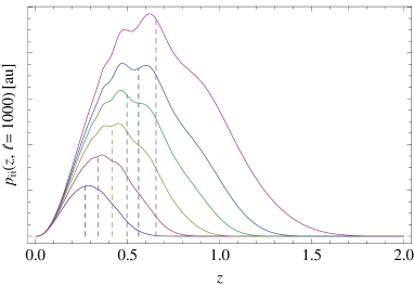
Figure 2: The integrand of Eq. (21). The curves from left to right correspond to $p_{ii}(z,\ell=1000)$, where $i=1,\dots,6$. The contribution to the lensing signal is very broad in redshift and peaks at relatively low $z$ even for the high-redshift bins. The median redshift for each curve is indicated by dashed lines. We give the median redshift for the lensing contribution in Table IV.

$\bar{z}$	$\ell_{{\rm max}}$	$z_{{\rm med}}$	$\bar{L}$	$\Delta\bar{L}$	$\Delta\bar{L}(\%)$	$E$	$\Delta E$	$\Delta E(\%)$
0.6	311	0.26	0.342	0.0044	1.3	1.37	0.0062	0.46
0.8	385	0.31	0.311	0.0044	1.4	1.53	0.0069	0.45
1.0	515	0.40	0.285	0.0059	2.1	1.72	0.017	0.96
1.2	609	0.45	0.262	0.0059	2.3	1.92	0.029	1.5
1.4	760	0.54	0.242	0.014	5.7	2.14	0.029	1.4
1.8	959	0.64	0.210	0.035	16	2.62	0.077	3.0

Table 5: Errors on $E$ and $\bar{L}$ from weak lensing only (with six redshift bins) and a list of the value $\ell_{{\rm max}}$ used at each redshift together with the corresponding $z_{{\rm med}}$ value.

To find the derivatives needed in Eq. (29), we divide the integral in Eq. (21) into $n_{B}$ integrals that each cover one redshift bin. We could assume that $\bar{L}(z)$ is constant across any redshift bin to get an approximate expression for the integral that depends on $\bar{L}$ in an analytical way, but the discrepancy between the actual integral and the approximate integral (and consequently the discrepancy of the derivative) can be up to a factor of 2, which may not be sufficient. Assuming that the integrand is linear in $z$ gives the same result (when using only the center of the bin as the sampling point), so the issue arises when the curvature of the integrand becomes large.

As a solution, we take the actual value of the integral and simply assume that it depends quadratically on $\bar{L}(\bar{z}_{a})$, such that the derivative can be written as

$$\frac{\partial P_{ij}(\ell)}{\partial\bar{L}(\bar{z}_{a})}=\frac{2}{\bar{L}(\bar{z}_{a})}\int_{z_{a}}^{z_{a+1}}p_{ij}(z,\ell)\mathrm{d}z.$$ (31)

Since $E$ appears in the comoving distance, it is more complicated for the derivatives of $P_{ij}$ with respect to $E(\bar{z}_{a})$. We substitute the regular definition of $E$ by an interpolating function that goes smoothly through all points $(\bar{z}_{a},E(\bar{z}_{a}))$ and $(0,1)$. Instead of depending on $\Omega_{m}$ it now depends on the values of all $E(\bar{z}_{a})$, and so do all functions that depend on $E$, in particular the comoving distance and consequently the window functions $K_{i}(z)$. The derivatives are then obtained by varying the fiducial values of $E(\bar{z}_{a})$ while keeping $L=\bar{L}\delta_{\text{t,0}}$ fixed so that we again do not include the derivative of $\delta_{\text{t,0}}^{2}$ with respect to $k$.

It is instructive to consider the error on the spectrum itself for a particular pair $ij$. If we take as parameters $p_{\alpha}=P_{ij}$ we have a variance

$$\sigma^{-2}=f_{{\rm sky}}\sum_{\ell}\Delta\ell\frac{(2\ell+1)}{2}C_{ij}^{-1}C_{ij}^{-1},$$ (32)

(no sum over $ij$) and neglecting the noise (appropriate for $\ell<500$) i.e. putting $C_{ij}=P_{ij}$, this becomes, in a small range of $\ell$ from $\ell_{\text{min}}$ to $\ell_{\text{max}}$ so that we can approximate $P_{ij}$ with a constant,

$$\sigma^{-2}P_{ij}P_{ij}=f_{{\rm sky}}\sum_{\ell}\Delta\ell\frac{(2\ell+1)}{2}=f_{{\rm sky}}\frac{\ell_{\text{max}}^{2}-\ell_{\text{min}}^{2}}{2},$$ (33)

(for $\ell_{\text{max,min}}\gg 1$). If $\ell_{\text{min}}$ is much smaller than $\ell_{\text{max}}$ this gives a relative error for every $ij$

$$\frac{\sigma}{P_{ij}}=\ell_{\text{max}}^{-1}\left(\frac{f_{{\rm sky}}}{2}\right)^{-1/2}\approx 2.3\,\ell_{\text{max}}^{-1},$$ (34)

so that for $\ell_{\text{max}}=300$ we should get a minimum relative error of $0.6\%$, which is indeed of the same order as our result. The error increases if we include the noise and a non-negligible $\ell_{\text{min}}$.

The resulting uncertainties on $E(\bar{z}_{a})$ and $\bar{L}(\bar{z}_{a})$ can be found in Table IV; they are visualized in Fig. 3.

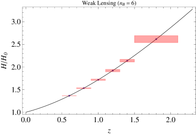
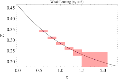
Figure 3: Errors on $E(\bar{z}_{a})$ (left) and $\bar{L}(\bar{z}_{a})$ (right) from weak lensing.

IV.1 $k$ binning

$\bar{z}$	$\ell_{0}$	$\ell_{1}$	$\ell_{2}$	$\ell_{3}$
0.6	6.3	39	120	410
0.8	7.9	45	190	610
1.0	9.4	66	240	880
1.2	11	83	320	1200
1.4	12	97	390	1500
1.8	14	120	550	2200

Table 6: Borders of the $\ell$-bins for each redshift bin converted from the $k$-bins according to Eq. (30).

To test the cases three and four of our models for $\eta$, we need to consider $\bar{L}$ as a function of $k$ (although with the same fiducial value for all $k$, as the fiducial model is $\Lambda$CDM), and we divide the full $k$-range again into the same three bins. The observables are then $\bar{L}_{an}\equiv\bar{L}(\bar{z}_{a},\bar{k}_{n})$, where $\bar{k}_{n}$ denote the center of the $k$-bins, with $n=1,2,3$. They are defined as in Sec. III, and are given explicitly in Table 1. The $k$-bins fix the ranges for $\ell$ via the relation used in Eq. (30). We label the center of the $\ell$-bins accordingly as $\ell_{n}$. See Table 6 for a list of the $\ell$-bins. The derivatives needed for the Fisher matrix will be evaluated at the center of these $\ell$-bins.

They can be computed similarly as in Eq. (31). We find (using Kronecker deltas, no summation):

$$\frac{\partial P_{ij}(\ell)}{\partial\bar{L}(\bar{z}_{a},k_{n})}=\frac{2\delta_{an}}{\bar{L}(z_{a})}\int_{z_{a}}^{z_{a+1}}p_{ij}(z,\ell)\mathrm{d}z\times\begin{cases}1&{\rm if}\quad\ell_{n-1}<\ell<\ell_{n}\\ 0&{\rm else}.\end{cases}$$ (35)

The derivatives with respect to $E(\bar{z}_{a})$ are computed the same way as before. We can then define the parameter vector $p_{\alpha}=\{\bar{L}_{11},E_{1},\bar{L}_{12},E_{1},\bar{L}_{13},E_{3},\bar{L}_{21},E_{2},...\}$ and evaluate the Fisher matrix formally as before. The structure of the Fisher matrix can be schematically represented as follows:

$$\left(\begin{array}[]{cccc}\bar{L}_{1}\bar{L}_{1}&0&0&\bar{L}_{1}E\\ 0&\bar{L}_{2}\bar{L}_{2}&0&\bar{L}_{2}E\\ 0&0&\bar{L}_{3}\bar{L}_{3}&\bar{L}_{3}E\\ \bar{L}_{1}E&\bar{L}_{2}E&\bar{L}_{3}E&EE\end{array}\right)$$ (36)

The uncertainties placed on the observables by weak lensing only can be found in Table IV.

Table 7: Errors of $\bar{L}_{ai}$ and $E$ using weak lensing only with their fiducial values.

V Supernovae

$\bar{z}$	$\sigma_{{\rm data},a}$	$n_{a}$	$E(\bar{z})$	$\Delta E$	$\Delta E(\%)$
0.6	0.287	46429	1.37	0.0026	0.19
0.8	0.285	25000	1.53	0.0041	0.27
1.0	0.329	16071	1.72	0.0086	0.50
1.2	0.327	7143	1.92	0.016	0.83
1.4	0.258	5357	2.14	0.028	1.3

Table 8: Redshift uncertainties, number of supernovae, fiducial value of $E$ and errors for each bin.

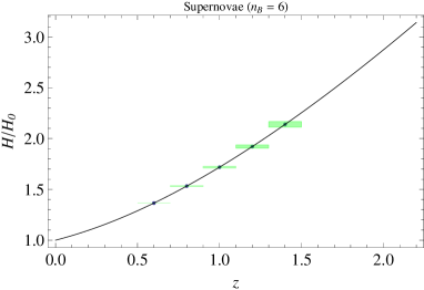
Figure 4: Errors on $E$ from Supernovae.

We consider now the forecasts for a supernovae survey. The likelihood function for the supernovae after marginalization of the offset is Amendola2010

$$\mathcal{L}=-\log L=\frac{1}{2}\left(S_{2}-\frac{S_{1}^{2}}{S_{0}}\right),$$ (37)

where

$$S_{n}=\sum_{i}\frac{(m_{i}-\mu_{i})^{n}}{\sigma_{i}^{2}},$$ (38)

and $\mu_{i}=5\log\hat{d}_{L}$, where $\hat{d}_{L}$ is the dimensionless luminosity distance, see Eq. (8). This can be written as

$$\mathcal{L}=\frac{1}{2}X_{i}M_{ij}X_{j},$$ (39)

where $X_{i}=m_{i}-\mu_{i}$ and

$$M_{ij}=s_{i}s_{j}\delta_{ij}-\frac{s_{i}^{2}s_{j}^{2}}{S_{0}},$$ (40)

(no sum) where $s_{i}=1/\sigma_{i}$. The Fisher matrix can be written as

$$F_{\alpha\beta}^{\text{SN}}=\left\langle\frac{\partial\mathcal{L}}{\partial p_{\alpha}}\frac{\partial\mathcal{L}}{\partial p_{\beta}}\right\rangle,$$ (41)

where now the parameters are $p_{\alpha_{a}}^{\text{\tiny{SN}}}=E(\bar{z}_{a})$. Similarly to section III we can write

$$\hat{d}_{L}(\bar{z}_{a})=(1+\bar{z}_{a})\sum_{b=0}^{b=a}\frac{\Delta z_{b}}{E(\bar{z}_{b})},$$ (42)

so that

$$\frac{\partial\hat{d}_{L}(z_{a})}{\partial E(\bar{z}_{b})}=-\frac{\Delta z_{b}}{E_{b}^{2}}(1+z_{a})\delta_{ab}$$ (43)

where $\delta_{ab}$ is a Kronecker symbol. The Fisher matrix for the parameter vector $p_{\alpha}=\{E(z_{a})\}$ with $a$ running over the $z$-bins is then

$$F_{\alpha\beta}^{\text{SN}}=\left\langle\left(\frac{\partial\mu_{i}}{\partial p_{\alpha_{a}}}M_{ij}X_{j}\right)\left(\frac{\partial\mu_{i}}{\partial p_{\beta_{b}}}M_{ij}X_{j}\right)\right\rangle=25Y_{i\alpha}M_{ij}Y_{j\beta}.$$ (44)

where

$$Y_{i\alpha}\equiv\frac{\partial\log\hat{d}_{L}(\bar{z}_{i})}{\partial p_{\alpha}}=\frac{1}{\hat{d}_{L}(\bar{z}_{i})}\frac{\partial\hat{d}_{L}(\bar{z}_{i})}{\partial E(\bar{z}_{\alpha})}=-\frac{1}{\hat{d}_{L}(z_{i})}\frac{\Delta\bar{z}_{\alpha}}{E_{\alpha}^{2}}(1+\bar{z}_{i})\delta_{i\alpha}.$$ (45)

We have to make a choice to define the redshifts $z_{i}$ and the uncertainties $\sigma_{i}$ for the supernovae of the simulated future experiment. We take the Union 2.1 catalog as a reference (580 SNIa in the range $0<z\lesssim 1.5$). We assume that the survey will observe supernovae in the redshift range $0.5<z<1.5$, and divide that interval in bins of fixed width $\Delta z=0.2$ just like in Sec. III, in order to combine the SN Fisher matrix with the galaxy clustering and the weak lensing ones. We assume the total number of observed SN to be about $n_{\text{SN}}=100000$ in that range, as expected for the LSST survey Tyson:2003kb . We further assume that the supernovae of the future survey will be distributed uniformly in each bin, respecting the proportions of the data of the catalog Union 2.1 and with the same average magnitude error. The values of $\sigma_{\text{data},a}$ and $n_{a}$ for the bins centered in $\bar{z}_{a}$ are summarized in Table 8.

Finally, the corresponding errors on $E$ from supernovae are shown in Fig. 4 and in Table 8. In Table IV we compare the errors on $E$ from the three different probes with each other. We notice that the supernova constraints are the most stringent ones among the three probes and improve the WL+GC constraints by almost a factor of two. All this of course assumes that systematic errors can be kept below statistical errors.

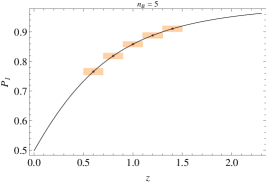
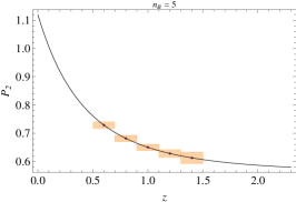
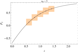
Figure 5: Errors on $P_{1}$, $P_{2}$ and $P_{3}$ in the $z$-varying case.

Table 9: Fiducial values and errors for the parameters $P_{1}$, $P_{2}$, $P_{3}$, $E^{\prime}/E$ and $\bar{\eta}$ for every bin. The last bin has been omitted since $R^{\prime}$ is not defined there.

Table 10: Same as Table IV, but with four redshift bins. The last bin has again been omitted.

VI Combining the matrices

Once we have the three Fisher matrices for galaxy clustering, weak lensing and supernovae, we insert them block-wise into a $(4n_{B})\times(4n_{B})$ matrix for the full parameter vector

$$p_{\alpha}=\{\bar{A},\bar{R},\bar{L},E\}\times n_{B},$$ (46)

Notice that we need also $\bar{R}^{\prime}=-(1+z)[\bar{R}(z+\Delta z)-\bar{R}(z)]/\Delta z$ and $E^{\prime}=-(1+z)[E(z+\Delta z)-E(z)]/\Delta z$. The full schematic structure for every bin will be:

$$\left(\begin{array}[]{cccc}\bar{A}\bar{A}&\bar{A}\bar{R}&0&\bar{A}E\\ \bar{A}\bar{R}&\bar{R}\bar{R}&0&\bar{R}E\\ 0&0&\bar{L}\bar{L}&\bar{L}E\\ \bar{A}E&\bar{R}E&\bar{L}E&(EE)^{\Sigma}\end{array}\right),$$ (51)

with $(EE)^{\Sigma}=(EE)^{\text{GC}}+(EE)^{\text{WL}}+(EE)^{\text{SN}}$. This matrix must then be projected onto $\bar{\eta}$. It is however interesting to produce two intermediate steps, namely the matrix for $q_{\alpha}=\{P_{1},P_{2},P_{3},E\}$ where $P_{1}=R/A$, $P_{2}=L/R$ and $P_{3}=R^{\prime}/R$, as well as the matrix for $q_{\alpha}=\{P_{1},P_{2},P_{3},E^{\prime}/E\}$. They are given by

$$F_{\alpha\beta}^{(q)}=F_{\gamma\delta}^{(p)}\frac{\partial p_{\gamma}}{\partial q_{\alpha}}\frac{\partial p_{\delta}}{\partial q_{\beta}}.$$ (52)

We then project onto $\{P_{1},P_{2},\bar{\eta},E\}$. In Table IV we present the fiducial values for the parameters $P_{1}$, $P_{2}$, $P_{3}$, defined in Sec. I; In Fig. 5 we plot their fiducial values and errors. Let us call this the basic Fisher matrix.

As we mentioned in the introduction, we decided to consider four models for $\bar{\eta}$: constant, variable only in redshift, variable both in space and redshift, and the Horndeski model. For the constant $\bar{\eta}$ case we project the basic Fisher Matrix for $P_{1},P_{2},\bar{\eta},E$ onto a single constant value for $\bar{\eta}$. The resulting uncertainty for $\bar{\eta}$ is 0.010 .

For the $z$-variable case we project on five $\bar{\eta}$ parameters, one for each bin. The results are in Table IV. We see that the error on $\bar{\eta}$ rises to around 10%. Without the SN data, the final constraints on $\eta$ would weaken only by roughly 1%. If we collect the data into only three wider $z$ bins, the error reduces to about 3%.

For the $z,k$ varying case, we consider the $k$-binning of Sec. III.2. Now the information is distributed over many more bins, so the errors obviously degrade (see Table IV). We find errors from 10% to more than 100%.

Finally, for the Horndeski case, Table IV gives the absolute errors on $h_{2},h_{4}$ (measuring $k$ in units of 0.1 $h/$Mpc). Here we are forced to fix $h_{5}$ to its fiducial value (i.e. to zero) due to the degeneracy between $h_{4}$ and $h_{4}$ when the fiducial model is such that $h_{4}=h_{5}$, as in the $\Lambda$CDM case. This means we are only able to measure the difference $h_{4}-h_{5}$ rather than the two functions separately. The absolute errors on $h_{2},h_{4}$ are in the range 0.2-0.6. This result implies for instance that, at a scale of 0.1 $h/$Mpc and in a redshift bin 0.5-0.7, a Euclid-like mission can detect the presence of a $k^{2}$ behavior in $\eta$ if it is larger than 60% than the $k$-independent trend (see Fig. 6 for a visualization of the constraints on $\eta$).

Table 11: Errors on $E$ from the three probes.

$\bar{z}$	$i$	$P_{1}$	$\Delta P_{1}$	$\Delta P_{1}(\%)$	$P_{2}$	$\Delta P_{2}$	$\Delta P_{2}(\%)$	$P_{3}$	$\Delta P_{3}$	$\Delta P_{3}(\%)$	$\bar{\eta}$	$\Delta\bar{\eta}$	$\Delta\bar{\eta}(\%)$
0.6	1	0.766	0.14	18	0.729	0.12	17	0.134	1.4	1100	1	1.1	120
	2		0.032	4.1		0.030	4.1		0.33	240		0.26	26
	3		0.013	1.7		0.015	2.0		0.15	110		0.12	12
0.8	1	0.819	0.11	13	0.682	0.092	13	0.317	1.2	380	1	0.93	93
	2		0.024	2.9		0.021	3.1		0.26	83		0.2	20
	3		0.011	1.4		0.013	1.9		0.14	43		0.1	10
1.0	1	0.859	0.093	11	0.65	0.076	12	0.46	1.1	240	1	0.82	82
	2		0.020	2.3		0.019	2.9		0.23	51		0.17	17
	3		0.011	1.2		0.012	1.8		0.14	31		0.1	11
1.2	1	0.888	0.084	9.4	0.628	0.074	12	0.569	1.1	190	1	0.78	78
	2		0.017	2.0		0.021	3.3		0.23	40		0.16	16
	3		0.011	1.2		0.017	2.7		0.17	29		0.12	12
1.4	1	0.911	0.079	8.7	0.613	0.084	14	0.654	0.79	120	1	0.55	55
	2		0.017	1.9		0.027	4.4		0.17	26		0.12	12
	3		0.013	1.4		0.023	3.8		0.14	21		0.094	9.4

Table 12: Here, the errors on $P_{1}$, $P_{2}$, $P_{3}$ and $\eta$ are listed for the $z,k$-varying case with a similar structure as Table 4.

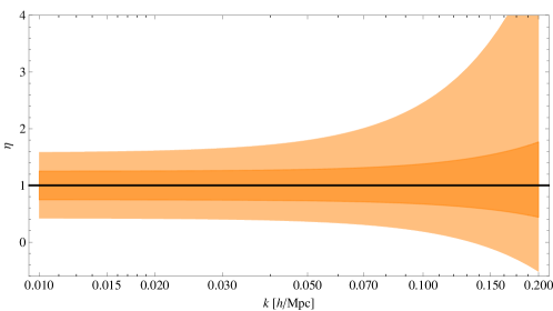
Figure 6: Constraints on $\eta(k)$ in the Horndeski case for $z=0.6$ (light) and $z=1.4$ (dark).

Table 13: Absolute errors on $h_{2}$ and $h_{4}$. Because of the degeneracy between $h_{5}$ and $h_{4}$, $h_{5}$ has been fixed. The fiducial values are $h_{2}=1$ and $h_{4}=0$.

VII Conclusions

In this paper we study the precision with which a future large survey of galaxy clustering and weak lensing like Euclid can determine the anisotropic stress of the dark sector with the help of the model-independent cosmological observables introduced in Amendola:2012ky , when augmented with a supernova survey.

We find that galaxy clustering and weak lensing will achieve precise measurements of the expansion rate $E(z)=H(z)/H_{0}$, with errors of less than a percent in redshift bins of $\Delta z=0.2$ out to $z=1.5$, and with less than 4% out to $z=2$, see Table IV.

They will also be able to measure $P_{1}=f/b$ to about a percent precision over the full redshift range (in the same bins), and achieve a comparable precision on $P_{2}=\Omega_{{\rm m,0}}\Sigma/f$, except at $z>1.5$ where the errors increase rapidly. The final quantity, $P_{3}=f+f^{\prime}/f$, is constrained much less precisely, only to about 30%, because it involves an explicit derivative. The detailed results are given in Tables IV and IV.

We then considered four different models for $\eta=-\Phi/\Psi$:

1. A constant $\eta$: In this case we find that we can determine the derived quantity $\bar{\eta}$ with a precision of about 1%.

2. $\eta$ varying with redshift, but not with scale: For bins with a size of $\Delta z=0.2$, we find a precision on $\bar{\eta}$ of about 10% out to $z=1.5$.

3. $\bar{\eta}$ varying both in $z$ and in $k$: the errors vary considerably across the $z,k$ range, from 10% to more than 100%.

4. The Horndeski case: now the absolute errors on $h_{2},h_{4}$ are in the range 0.2-0.6

We stress again that in this paper we used only directly observable quantities without any further assumptions about the initial power spectrum, the dark matter, the dark energy model (beyond the behaviour of $\eta$ in the last step) or the bias, as such assumptions may be unwarranted in a general dark energy or modified gravity context. On the other hand, we do assume that a window between non-linear scales and sub-sound-horizon scales exists and is wide enough to cover all the wavelengths we have been employing in our forecasts.

Appendix A Sampling vs Fisher matrix analysis

In order to check whether the Fisher matrix analysis is appropriate for the non-linear parameter combinations that make up the $P_{i}$ and $\eta$ we also use an alternative approach. We assume that the Fisher matrix forecast for the errors on $\bar{A}$, $\bar{R}$, $\bar{L}$ and $E$ is sufficiently accurate (i.e. that the joint posterior of these variables can be described by a Gaussian probability distribution function with the covariance matrix given by the inverse of the Fisher matrix), which should be a reasonable assumption given how precise the surveys that we consider here are. We then draw random samples from the multivariate Gaussian distribution defined by those Fisher matrices.

For each sample we compute $P_{1}$, $P_{2}$ and $P_{3}$ at the corresponding values of $z$ and $k$. We compute the derivatives of $E$ and $\bar{R}$ by fitting a cubic spline through each realisation of $E(z)$ and $\bar{R}(z)$ and calculating the derivative of the spline. This procedure allows us to obtain estimates of the derivatives in all bins, but at the price of having to choose boundary conditions for the splines (we use the “natural spline” convention that the second derivative vanishes at the boundary).

Overall we find good agreement, and even excellent agreement when using the derivative at the points in between the bins (which agrees better with the finite difference method used for the Fisher forecasts). The agreement becomes much worse for $\eta$, as already mentioned in the introduction. This is however no surprise, as the posterior distribution of $\eta$ becomes very non-Gaussian for the survey specifications considered here (while the posterior distributions of the $P_{i}$ remain close to Gaussian). We observe however that $\bar{\eta}$ retains a normal posterior, which makes it much better suited for the Fisher forecast approach, see Fig. 7. The same holds true for Markov-Chain Monte Carlo approaches which tend to have difficulties with sampling from curved, “banana-shaped” posteriors, and so we recommend quite generally to use $\bar{\eta}$ rather than $\eta$ in data analysis. We finally note that when $\eta$ is well-constrained and has a pdf close to Gaussian, then its standard deviation should be about twice that of $\bar{\eta}$.

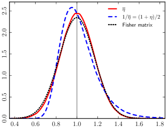
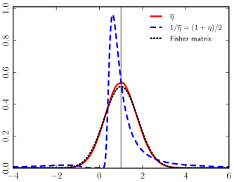
Figure 7: The probability density function (pdf) for $(1+\eta)/2$ (blue dashed line) and $\bar{\eta}$ (red solid line) based on sampling from the Fisher matrix for $\{\bar{A},\bar{R},\bar{L},E\}$, compared to the Gaussian pdf from the Fisher matrix projection on $\bar{\eta}$ (black dotted line) in the $z$- and $k$-binning case. The left panel shows the second $k$-bin for $\bar{z}=1$, and the right panel the first $k$-bin for $\bar{z}=1.2$. We use $(1+\eta)/2$ instead of $\eta$ because it has the same pdf shape as $\eta$ and (to lowest order) the same variance as $\bar{\eta}$. We see that even when the standard deviation of $\bar{\eta}$ is well below $1$ as in the left panel, the pdf of $\eta$ is significantly less Gaussian than the pdf of $\bar{\eta}$. For large standard deviation (right panel) the pdf of $\bar{\eta}$ is still well behaved and close to Gaussian, while the one of $\eta$ is strongly distorted and exhibits large tails (not shown in the figure) due to a division by zero problem in the expression (4).

References

- (1) Planck Collaboration Collaboration, P. Ade et al., “Planck 2013 results. I. Overview of products and scientific results,” arXiv:1303.5062 [astro-ph.CO].
- (2) Planck Collaboration Collaboration, P. Ade et al., “Planck 2013 results. XVI. Cosmological parameters,” arXiv:1303.5076 [astro-ph.CO].
- (3) L. Amendola, M. Kunz, M. Motta, I. D. Saltas, and I. Sawicki, “Observables and unobservables in dark energy cosmologies,” Phys.Rev. D87 (2013) 023501, arXiv:1210.0439 [astro-ph.CO].
- (4) L. Amendola, M. Kunz, and D. Sapone, “Measuring the dark side (with weak lensing),” JCAP 0804 (2008) 013, arXiv:0704.2421 [astro-ph].
- (5) A. De Felice, T. Kobayashi, and S. Tsujikawa, “Effective gravitational couplings for cosmological perturbations in the most general scalar-tensor theories with second-order field equations,” Phys.Lett. B706 (2011) 123–133, arXiv:1108.4242 [gr-qc].
- (6) I. D. Saltas and M. Kunz, “Anisotropic stress and stability in modified gravity models,” Phys.Rev. D83 (2011) 064042, arXiv:1012.3171 [gr-qc].
- (7) I. Sawicki, I. D. Saltas, L. Amendola, and M. Kunz, “Consistent perturbations in an imperfect fluid,” JCAP 1301 (2013) 004, arXiv:1208.4855 [astro-ph.CO].
- (8) M. Motta, I. Sawicki, I. D. Saltas, L. Amendola, and M. Kunz, “Probing Dark Energy through Scale Dependence,” arXiv:1305.0008 [astro-ph.CO].
- (9) M. Kunz, “The dark degeneracy: On the number and nature of dark components,” Phys.Rev. D80 (2009) 123001, arXiv:astro-ph/0702615 [astro-ph].
- (10) G. Ballesteros, L. Hollenstein, R. K. Jain, and M. Kunz, “Nonlinear cosmological consistency relations and effective matter stresses,” JCAP 1205 (2012) 038, arXiv:1112.4837 [astro-ph.CO].
- (11) A. Albrecht, G. Bernstein, R. Cahn, W. L. Freedman, J. Hewitt, et al., “Report of the Dark Energy Task Force,” arXiv:astro-ph/0609591 [astro-ph].
- (12) R. Laureijs, J. Amiaux, S. Arduini, J. . Auguères, J. Brinchmann, R. Cole, M. Cropper, C. Dabin, L. Duvet, A. Ealet, and et al., “Euclid Definition Study Report,” ArXiv e-prints (Oct., 2011) , arXiv:1110.3193 [astro-ph.CO].
- (13) LSST Collaboration Collaboration, J. A. Tyson, “Large synoptic survey telescope: Overview,” Proc.SPIE Int.Soc.Opt.Eng. 4836 (2002) 10–20, arXiv:astro-ph/0302102 [astro-ph].
- (14) H.-J. J. Seo and D. J. Eisenstein, “Probing dark energy with baryonic acoustic oscillations from future large galaxy redshift surveys,” Astrophys.J 598 (2003) 720–740, arXiv:0307460 [astro-ph].
- (15) C. Alcock and B. Paczynski, “An evolution free test for non-zero cosmological constant,” Nature (London) 281 (Oct., 1979) 358.
- (16) L. Amendola and S. Tsujikawa, Dark Energy: Theory and Observations. Cambridge University Press, 2010.
- (17) Euclid Theory Working Group Collaboration, L. Amendola et al., “Cosmology and fundamental physics with the Euclid satellite,” arXiv:1206.1225 [astro-ph.CO].
- (18) A. Lewis, A. Challinor, and A. A. Lasenby, “Efficient Computation of CMB anisotropies in closed FRW models,” Astrophys.J. 538 (2000) 473–476, arXiv:9911177 [astro-ph]. Code available in http://camb.info/.
- (19) A. Orsi, C. Baugh, C. Lacey, A. Cimatti, Y. Wang, et al., “Probing dark energy with future redshift surveys: A comparison of emission line and broad band selection in the near infrared,” arXiv:0911.0669 [astro-ph.CO].
- (20) W. Hu, “Power spectrum tomography with weak lensing,” Astrophys.J. 522 (1999) L21–L24, arXiv:astro-ph/9904153 [astro-ph].
- (21) Z. Ma, W. Hu, and D. Huterer, “Effects of Photometric Redshift Uncertainties on Weak-Lensing Tomography,” Astrophys. J. 636 (Jan., 2006) 21–29, arXiv:0506614 [astro-ph].
- (22) D. J. Eisenstein, W. Hu, and M. Tegmark, “Cosmic Complementarity: Joint Parameter Estimation from Cosmic Microwave Background Experiments and Redshift Surveys,” Astrophys. J. 518 (June, 1999) 2–23, astro-ph/9807130.