Approximation Algorithms for Hard Capacitated $k$-facility Location Problems

Abstract

We study the capacitated $k$-facility location problem, in which we are given a set of clients with demands, a set of facilities with capacities and a constant number $k$. It costs $f_{i}$ to open facility $i$, and $c_{ij}$ for facility $i$ to serve one unit of demand from client $j$. The objective is to open at most $k$ facilities serving all the demands and satisfying the capacity constraints while minimizing the sum of service and opening costs.

In this paper, we give the first fully polynomial time approximation scheme (FPTAS) for the single-sink (single-client) capacitated $k$-facility location problem. Then, we show that the capacitated $k$-facility location problem with uniform capacities is solvable in polynomial time if the number of clients is fixed by reducing it to a collection of transportation problems. Third, we analyze the structure of extreme point solutions, and examine the efficiency of this structure in designing approximation algorithms for capacitated $k$-facility location problems. Finally, we extend our results to obtain an improved approximation algorithm for the capacitated facility location problem with uniform opening cost.

1 Introduction

In the capacitated $k$-facility location problem (CKFL), we are given a set $D$ of clients and a set $F$ of potential facilities (locations where we can potentially open a facility) in a metric space. Each facility $i\in F$ has a capacity $s_{i}$. Each client $j$ has a demand $d_{j}$ that must be served. Establishing facility $i$ incurs an opening cost $f_{i}$. Shipping $x_{ij}$ units from facility $i$ to client $j$ incurs service costs $c_{ij}x_{ij}$, where $c_{ij}$ is proportional to the distance between $i$ and $j$. The goal is to serve all the clients by using at most $k$ facilities and satisfying the capacity constraints such that the total cost is minimized. In this paper, we consider the hard capacities, that is, we allow at most one facility to be opened at any location. (Note that in the soft capacities case multiple facilities can be opened in a single location [33].)

CKFL can be formulated as the following mixed integer program (MIP), where variable $x_{ij}$ indicates the amount of the demand of client $j$ that is served by facility $i$, and $y_{i}$ indicates whether facility $i$ is open.

$$\min\quad \sum_{i\in F}\sum_{j\in D}c_{ij}x_{ij}+\sum_{i\in F}f_{i}y_{i}$$ (1)

subject to: $$\sum_{i\in F}{x_{ij}}=d_{j}, \forall j\in D,$$ (2)

$$\sum_{j\in D}{x_{ij}}\leq s_{i}y_{i}, \forall i\in F,$$ (3)

$$\sum_{i\in F}{y_{i}}\leq k,$$ (4)

$$x_{ij}\geq 0, \forall i\in F,\forall j\in D,$$ (5)

$$y_{i}\in\{0,1\}, \forall i\in F.$$ (6)

If we replace constraints (6) by

$$0\leq y_{i}\leq 1,i\in F,$$ (7)

we obtain the LP-relaxation of CKFL. Without loss of generality we suppose that $s_{i}$, $d_{j}$ for each $i\in F,j\in D$ are all integral.

CKFL is related to the capacitated $k$-median problem (CKM), in which inputs and goal are the same as CKFL except that there is no opening cost for facilities. A constant factor approximation algorithm is still unknown for CKM, let alone CKFL. All the previous attempts with constant approximation ratios for these problems violate the capacity constraint, or cardinality constraint that at most $k$ facilities are allowed to be used. We call these approximation algorithms pesudo-approximation algorithms. Recently, Byrka et al. [7] gave a constant factor approximation algorithm for CKM with uniform capacities while violating the capacities with a factor $2+\epsilon$, where $\epsilon>0$ can be arbitrarily small. Although most researchers believe that relaxing the cardinality constraint makes the problem simpler than relaxing the capacity constraint with respect to designing pesudo-approximation algorithms, the best known violation ratio for cardinality constraint is still $5+\epsilon$ to get a constant factor approximation algorithm [27] for CKM with uniform capacities. It seems that to obtain a better constant factor approximation algorithm with violating the cardinality constraint has not received much attention yet.

In this paper, we give an improved approximation algorithm for CKFL (with arbitrary capacities) with uniform opening cost by using at most $2k$ facilities. To show the potential power of this algorithm, we improve the approximation ratio for the capacitated facility location problem with uniform opening cost [30], by combining this algorithm with a pesudo-approximation algorithm for the $k$-median problem derived from a bifactor approximation algorithm for the uncapacitated facility location problem [10]. That is, pesudo-approximation algorithms for capacitated $k$-facility location problems may be extended to get approximation algorithms for well-studied capacitated facility location problems. We believe that this technique has the potential to further improve approximation ratios for capacitated facility location problems.

Additionally, in Section 2 we give the first fully polynomial time approximation scheme (FPTAS) for the single-sink (hard) capacitated $k$-facility location problem. In Section 3, we give a polynomial time algorithm for the uniform capacitated $k$-facility location problem with a fixed number of clients.

1.1 Related Work

The $k$-facility location problem has already been studied since the early 90s [14, 21]. It is a common generalization of the $k$-median problem (in which at most $k$ facilities are allowed to be opened, and there is no opening costs) and the uncapacitated facility location problem, which are classical problems in computer science and operations research and have a wide variety of applications in clustering, data mining, logistics [6, 22, 28], even for the single-sink (single client) case [19].

For the uncapacitated $k$-facility location problem (UKFL), Charikar et al. [11] gave the first constant factor approximation algorithm with performance guarantee 9.8, by modifying their $6\tfrac{2}{3}$-approximation algorithm for the uncapacitated $k$-median problem. Later, the approximation ratio was improved by Jain and Vazirani [25], who made use of a primal-dual scheme and Lagrangian relaxation techniques to obtain a $6$-approximation algorithm. Jain et al. [23, 24] further improved the ratio to $4$ by using a greedy approach and the so-called Lagrangian Multiplier Preserving property of the algorithms. The best known approximation algorithm for this problem, due to Zhang [38], achieves a factor of $2+\sqrt{3}+\epsilon$ using a local search technique. The $k$-median problem, as a special case of UKFL, was studied extensively [2, 3, 8, 10, 11, 24, 25, 31] and the best known approximation algorithm was recently given by Byrka et al. [8] with approximation ratio $2.611+\epsilon$ by improving the algorithm of Li and Svensson [31]. In addition, Edwards [15] gave a $7.814$-approximation algorithm for the multi-level uncapacitated $k$-facility location problem by extending the $6\frac{2}{3}$-approximation algorithm by Charikar et al. [11] for the uncapacitated $k$-median problem.

Unfortunately, the capacitated $k$-facility location problem is much less understood although the presence of capacity constraints is natural in practice. The difficulty of the problem lies in the fact that two kinds of hard constraints appear together: the cardinality constraint, and the capacity constraints. This seems to result in hardness of the methods such as LP-rounding, primal-dual method used to solve the $k$-median problem, and even local search algorithms used to solve the capacitated facility location problem and the $k$-median problem.

The capacitated $k$-facility location problem is related to the capacitated facility location problem (CFL), whose inputs and goal are the same as for CKFL but without the cardinality constraint. Most known approximation algorithms for CFL are based on local search technique since the natural linear programming relaxation has an unbounded integrality gap for the general case [34]. For nonuniform capacities, Pál, Tardos, and Wexler [34] proposed the first constant factor approximation algorithm with a factor of $8.53$. Later, Mahdian and Pál [32] improved this factor to $7.88$. Zhang, Chen, and Ye [37] reduced this factor to $(3+2\sqrt{2}+\varepsilon)$ by introducing a multi-exchange operation. The currently best known approximation algorithm, due to Bansal, Garg, and Gupta [4], achieves the approximation ratio $5$. As it was expected that the problem is easier for uniform capacities, Korupolu, Plaxton, and Rajaraman (KPR) [27] gave the first constant factor approximation algorithm with a factor of $8$. Later, this factor was improved to $5.83$ by Chudak and Williamson [12]. The currently best approximation algorithm due to Aggarwal et al. [1] has performance guarantee of 3.

Additionally, Levi, Shmoys, and Swamy [30] showed that the linear programming relaxation has a bounded integrality gap for CFL with uniform opening costs, and gave a $5$-approximation algorithm for this case by an LP-rounding technique.

The capacitated $k$-median problem (CKM), which is a special case of CKFL, is already difficult to handle. The natural linear programming relaxation has an unbounded integrality gap (see Remark 1). We have to blow up the capacity or increase the number of opening facilities by a factor of at least 2 if we use the cost of the LP solution as a lower bound to obtain an integral solution [11].

For the hard uniform capacity case, Charikar et al. [11] gave a constant factor approximation algorithm while violating the capacities within a constant factor $3$ by LP-rounding. Recently, Byrka et al. [7] improved this violation ratio to $2+\epsilon$ by designing a $(32l^{2}+28l+7)$-approximation algorithm increasing the capacity by a factor of $2+\frac{3}{l-1}$, $l\in\{2,3,4,\cdots\}$. Based on a local search technique, Korupolu et al. [27] proposed a $(1+{5}/{\epsilon})$-approximation algorithm by using at most $(5+\epsilon)k$ facilities, and a $(1+{\epsilon})$-approximation algorithm by using at most $(5+5/\epsilon)k$ facilities.

For soft non-uniform capacities, based on primal-dual and Lagrangian relaxation methods, Chuzhoy and Rabani [13] presented a $40$-approximation algorithm by violating the capacities within a constant factor of $50$. Bartal et al. [5] proposed a $19.3(1+\delta)/\delta^{2}$-approximation algorithm ($\delta>0$) by using at most $(1+\delta)k$ facilities.

To the best of our knowledge, for hard non-uniform capacities, a constant factor approximation algorithm is still unknown if we allow for a violation of the two kinds of hard constraints: the cardinality constraint and capacity constraints. Without violating any constraint, a constant factor approximation algorithm remains unknown even for the single-sink capacitated $k$-median problem in which $|D|=1$, let alone the capacitated $k$-facility location problem.

1.2 Our Contributions and Techniques

(i) The single-sink facility location problem has several applications in practice [19]. We show that the single-sink hard capacitated $k$-facility location problem, in which $D$ contains exactly one client, is NP-hard even when $f_{i}=0,i\in F$. We give the first FPTAS for SCKFL by extending the FPTAS for the knapsack problem. To the best of our knowledge, this is also the fist FPTAS for the single-sink capacitated facility location problem, which answers a question by Görtz and Klose [17].

(ii) For the hard capacitated $k$-facility location problem with uniform capacities, in which $s_{i}=s,i\in F$, we observe that for $|D|$=1, it is easy to find an optimal solution. A natural question is to extend this to any fixed number $m:=|D|$ of clients. We give a polynomial time algorithm for this setting that runs in time $O({\binom{n}{m}}\cdot n^{3})$, where $n=|F|$. Using the structure of the graph consisting of the fractional valued edges in any extreme solution, the problem is reduced to a number of transportation problems.

(iii) We observe that the number of fractionally open facilities can be bounded by analyzing the rank of the constraint matrix corresponding to the tight constraints at a fractional extreme point solution. Then, we give approximation algorithms for two variants of the hard capacitated $k$-facility location problem based on this upper bound.

Another example to show the potential power of the structure of extreme point solutions is that we can slightly improve the previous best approximation ratio 5 obtained by Levi, Shmoys, and Swamy [30], and Bansal, Garg, and Gupta [4] for the capacitated facility location problem with uniform opening costs, by combining our technique with a pesudo-approximation algorithm for the $k$-median problem.

2 The Single-sink Capacitated $k$-facility Location Problem

In this section, we consider the single-sink capacitated $k$-facility location problem (SCKF). Since we only have one client with demand $d$, the formulation for the CKF is reduced to the following mixed integer program.

$$Z_{\mathrm{MIP}}=\min \sum_{i\in F}{(c_{i}x_{i}+f_{i}y_{i})}$$ (8)

subject to: $$\sum_{i\in F}{x_{i}}=d,$$ (9)

$$\sum_{i\in F}{y_{i}}\leq k,$$ (10)

$$0\leq{x_{i}}\leq s_{i}y_{i}, \forall i\in F,$$ (11)

$$y_{i}\in\{0,1\}, \forall i\in F.$$ (12)

Again, the natural LP relaxation of SCKFL can be obtained by replacing constraints (12) by (7).

Lemma 1.

The single-sink capacitated $k$-facility location problem is NP-hard even when $f_{i}=0$ for all $i\in F$.

Proof.

Consider the case that $s_{i}>1$, $c_{i}:=1-\frac{1}{s_{i}}$ and $f_{i}=0$ for all $i\in F$. We claim that

$$Z_{\mathrm{MIP}}\leq d-k\iff\text{there exists $I\subseteq F$ with $|I|=k$ and $\sum_{i\in I}s_{i}=d.$}$$ (13)

Indeed, for the objective value we find

$$\sum_{i\in F}{c_{i}x_{i}}=d-\sum_{i\in F}{\frac{x_{i}}{s_{i}}}=d-\sum_{i\mid y_{i}=1}\frac{x_{i}}{s_{i}}\geq d-k,$$

where the last inequality holds because $x_{i}\leq s_{i}$ and $y_{i}=1$ for $k$ values of $i$. Equality holds if and only if $x_{i}=s_{i}$ for all $i\in F$ with $y_{i}=1$. That is, if and only if $\sum\{s_{i}\mid y_{i}=1\}=d$.

The claim above allows to reduce SUBSET-SUM to SCKFL as follows. Let positive integers $s_{1},\cdots,s_{n}>1$ and $d$ form an instance of SUBSET-SUM. Now there exists a subset $I\subseteq\{1,2,\cdots,n\}$ such that $\sum_{i\in I}{s_{i}}=d$ if and only if the objective value of SCKFL is at most $d-k$ for some $k\in\{1,\cdots,n\}$. ∎

Remark 1.

The integrality gap $Z_{\mathrm{MIP}}/Z_{\mathrm{LP}}$ is unbounded.

Take the instance shown in Figure 1 with four facilities $\{1,2,3,4\}$, $s_{1}=s_{2}=s,s_{3}=Ms,s_{4}=s+1$, $d=2s+1$, $f_{1}=f_{2}=f_{3}=f_{4}=0$, and $c_{1}=c_{2}=0,c_{3}=100,c_{4}=1,k=2$ and $M\gg s\gg 100$. For this instance, we have $Z_{\mathrm{MIP}}=s+1$ and $Z_{\mathrm{LP}}=\frac{100M}{M-1}$. Thus, $Z_{\mathrm{MIP}}/Z_{\mathrm{LP}}=\frac{s+1}{\frac{100M}{M-1}}>\frac{s+1}{200}$, which can be arbitrarily large. In addition, a simple LP-rounding technique does not work for SCKFL. For the above instance, an optimal solution for LP-relaxation is $y_{1}=1,y_{2}=\frac{Ms-s-1}{(M-1)s},y_{3}=\frac{1}{(M-1)s},x_{1}=s,x_{2}=\frac{Ms-s-1}{M-1},x_{3}=\frac{M}{M-1}$. A natural idea is to round $y_{3}$ to be $1$, $y_{2}$ to be $0$. It is clear that the objective value of the solution obtained by this simple rounding is still really large.

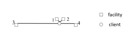
Figure 1: An instance for SCKFL. An optimal solution for the LP-relaxation of this instance is $y_{1}=1,y_{2}=\frac{Ms-s-1}{(M-1)s},y_{3}=\frac{1}{(M-1)s},x_{1}=s,x_{2}=\frac{Ms-s-1}{M-1},x_{3}=\frac{M}{M-1}$, with the total cost $\frac{100M}{M-1}$. An optimal solution for the MIP is $y_{1}=y_{4}=1,x_{1}=s,x_{4}=s+1$ with the total cost $s+1$.

We aim to design a fully polynomial time approximation scheme (FPTAS) for SCKFL. Before introducing our algorithm, we present a key observation (Pál, Tardos, and Wexler gave a similar observation in the proof of Lemma 3.3 in [34]).

Observation 1.

For the single-sink capacitated $k$-facility location problem, there is an optimal solution $(x^{*},y^{*})$ in which at most one open facility $t^{0}$ is not fully used, i.e., $x^{*}_{i}\in\{0,s_{i}\}$ for $i\neq t^{0}$.

Without loss of generality we suppose that $c_{ij}$ and $f_{i}$, for each $i\in F,j\in D$, are all integral. Given $t^{0}$, which is allowed not to be fully used in an optimal integral solution $(x^{*},y^{*})$, in order to solve SCKFL it is sufficient to solve the following problem for a given integer $p$:

$$\max\big{\{}\sum_{i\in F^{\prime}}s_{i}\mid F^{\prime}\subseteq F\setminus\{t^{0}\},|F^{\prime}|\leq k-1,\sum_{i\in F^{\prime}}(c_{i}s_{i}+f_{i})=p\big{\}}.$$ (14)

In words, we find for each total cost $p$ a set of at most $k-1$ facilities (not containing $t^{0}$) to open and use to full capacity, maximizing the total capacity.

We can recursively solve the above problem by dynamic programming. Without loss of generality, suppose $F\setminus\{t^{0}\}=\{1,2,\cdots,n-1\}$, where $n=|F|$. For nonnegative integers $p$ and $g\leq b\leq n-1$ define

$$S_{g}(b,p):=\max\big{\{}\sum_{i\in F^{\prime}}s_{i}\mid F^{\prime}\subseteq\{1,\ldots,b\},|F^{\prime}|\leq g,\sum_{i\in F^{\prime}}(c_{i}s_{i}+f_{i})=p\big{\}},$$

and let $F_{g}(b,p)$ be an optimal solution $F^{\prime}$. If $\sum_{i\in F^{\prime}}(c_{i}s_{i}+f_{i})=p$ does not hold for any $F^{\prime}\subseteq\{1,\ldots,b\}$ with $|F^{\prime}|\leq g$, we set $S_{g}(b,p):=-\infty$ and $F_{g}(b,p):=\emptyset$. Clearly, $S_{g}(0,0)=0$ and $S_{g}(0,p)=-\infty$ for $p>0$. The other values $S_{g}(b,p)$, and the corresponding optimum solutions $F_{g}(b,p)$, can be computed recursively since

$$S_{g}(b+1,p)=\max\big{(}S_{g}(b,p),\ s_{b+1}+S_{g-1}(b,p-(f_{b+1}+c_{b+1}s_{b+1})\big{)}$$

for $0<g\leq b$. In the maximum, the two values correspond to not opening and opening facility $b+1$, respectively.

For computing the maximum in (14), it suffices to restrict to values $0\leq p\leq(k-1)\mathcal{P}\leq n\mathcal{P}$, where $\mathcal{P}=\max\{c_{i}s_{i}+f_{i}\mid i\in\{1,\ldots,n-1\}\}$. Hence we can solve (14) in time $O(n^{3}\mathcal{P})$.

Since $\mathcal{P}$ may be exponential in the size of the input of SCKFL, the computing time could be non-polynomial. We overcome this difficulty by a scaling-and-rounding technique. The resulting Algorithm 1 may be seen as a generalization of the FPTAS for the knapsack problem (with cardinality constraints) [9, 29].

Assumption 1.

For each $i\in F,C_{i}>0$, where $C_{i}:=c_{i}s_{i}+f_{i}$.

Note that if $C_{i}=0$ and $s_{i}<d$ we directly open $i$ and serve demand $s_{i}$ of the single client by $i$ without increasing any cost. If $C_{i}=0$ and $s_{i}\geq d$, the optimal total cost is 0.

Algorithm 1 An FPTAS for the single sink capacitated $k$-facility location problem

Input

Finite set $F$ of facilities, costs $c\in\mathbb{Z}_{\geq 0}^{F}$, costs $f\in\mathbb{Z}_{\geq 0}^{F}$, demand $d\in\mathbb{Z}_{\geq 0}$, capacities $s\in\mathbb{Z}_{\geq 0}^{F}$, integer $1\leq k\leq n:=|F|$, $\epsilon>0$.

Output

A feasible solution $(x,y)$ that is within a factor $1+\epsilon$ of optimum, if a feasible solution exists.

Description

• Order facilities such that $C_{1}\leq C_{2}\leq\cdots\leq C_{n}$, where $C_{i}:=c_{i}s_{i}+f_{i}$.

• for $t=1$ to $n$ do

• for $r=1$ to $n$ do

• if $\{1,\cdots,r\}-\{t\}=\emptyset$,

• Let $C_{r}^{0}=0,$ $\bar{f}_{t}={f_{t}}$, $\bar{c}_{t}={c_{t}}$, $W=1$.

• end if

• if $\{1,\cdots,r\}-\{t\}\neq\emptyset$

• Let $W=\frac{\epsilon C_{r}^{0}}{k}$, where $C_{r}^{0}=\max\{C_{i}\mid i\in\{1,\cdots,r\}-\{t\}\}$.

• For each facility $i\in\{1,\cdots,r\}-\{t\}$, define $\bar{C}_{i}=\lfloor\frac{C_{i}}{W}\rfloor$.

• Let $\bar{f}_{t}=\frac{f_{t}}{W}$, $\bar{c}_{t}=\frac{c_{t}}{W}$.

• end if

• Consider the subproblem $P_{rt}$ involving items $\{1,\cdots,r\}\cup\{t\}$, in which

• only $t$ can be not fully used, that is, $x_{i}\in\{0,s_{i}\},i\in\{1,\cdots,r\}-\{t\}$;

• $0\leq x_{t}\leq s_{t}$. With the above scaled costs, compute $S_{g}(\bar{r},p)$ for each

• $0\leq g\leq k-1$, $0\leq p\leq(k-1)\lfloor\frac{C_{r}^{0}}{W}\rfloor$, where $\bar{r}=r$ if $r\neq t$, $\bar{r}=r-1$

• otherwise. Then, find a solution with total scaled cost:

• $\min\{p+(d-S_{g}(\bar{r},p))\bar{c}_{t}+\bar{f}_{t}\mid 0\leq d-S_{g}(\bar{r},p)\leq s_{t},0\leq g\leq k-1,$

• $0\leq p\leq(k-1)\lfloor\frac{C_{r}^{0}}{W}\rfloor\},$ if a feasible solution exists.

• end for

• end for

• for $r=1$ to $n$ do

• if $s_{r}\geq d$,

• find a solution with total cost $dc_{r}+f_{r}$.

• end if

• end for

• Output the solution with the minimum total original cost.

Remark 2.

Note that in Algorithm 1 for nonnegative integers $p$ and $g\leq b\leq\bar{r}$,

$$S_{g}(b,p):=\max\big{\{}\sum_{i\in F^{\prime}}s_{i}\mid F^{\prime}\subseteq\{1,\ldots,b\}-\{t\},|F^{\prime}|\leq g,\sum_{i\in F^{\prime}}(c_{i}s_{i}+f_{i})=p\big{\}}.$$

Theorem 1.

Let $OPT$ be the cost of an optimal solution, $SOL$ be the cost of the solution returned by Algorithm 1. Then, $SOL\leq(1+\epsilon)OPT$. The running time of Algorithm 1 is $O(\frac{n^{6}}{\epsilon})$, for any $\epsilon>0$.

Proof.

Suppose $(x^{*},y^{*})$ is an optimal solution in which at most one open facility is not fully used. Let $t^{0}$ be the open facility in $(x^{*},y^{*})$ that is not fully used if it exists. Otherwise, let $t^{0}$ be some open facility in $(x^{*},y^{*})$. Then, we define $F^{*}_{1}=\{i\in F\mid y^{*}_{i}=1\}-\{t^{0}\}$ as the set of opened facilities in $(x^{*},y^{*})$ excluding $t^{0}.$

If $F^{*}_{1}=\emptyset$, clearly our algorithm can find an optimal solution in Step 3. If $F^{*}_{1}\neq\emptyset$, let $C_{i}^{0}=\max\{C_{i}\mid i\neq t^{0},y^{*}_{i}=1\}$. Note that $C_{i}^{0}\leq OPT$. Moreover, let $i^{0}=\max\{i\in F^{*}_{1}\mid C_{i}=C_{i}^{0}\}$. Thus, $C_{i^{0}}=C_{i}^{0}.$

Suppose in iteration $t=t^{0},r=i^{0}$ of Step 2 we get an optimal solution $(x,y)$. Let $F_{1}=\{i\in F\mid y_{i}=1\}-\{t^{0}\}.$ Let $Cost(x,y)$ and $Scaled\_cost(x,y)$ be the original and scaled total cost of solution $(x,y)$ respectively. So, $Cost(x,y)=(\sum_{i\in F_{1}}{C_{i}})+x_{t^{0}}c_{t^{0}}+f_{t^{0}}$, and $Scaled\_cost(x,y)=(\sum_{i\in F_{1}}{\bar{C}_{i}})+x_{t^{0}}\bar{c}_{t^{0}}+\bar{f}_{t^{0}},$ where the definition of $\bar{C}_{i}$ is given in Algorithm 1. We will show that $Cost(x,y)\leq(1+\epsilon)OPT$, which then implies $SOL\leq(1+\epsilon)OPT$.

Recall that $W=\frac{\epsilon C_{r}^{0}}{k}$. We have

$$Cost(x,y) =(\sum_{i\in F_{1}}{C_{i}})+x_{t^{0}}c_{t^{0}}+f_{t^{0}}$$

$$\leq(\sum_{i\in F_{1}}{(W\bar{C}_{i}+W)})+Wx_{t^{0}}\bar{c}_{t^{0}}+W\bar{f}_{t^{0}}$$

$$\leq W((\sum_{i\in F_{1}}{\bar{C}_{i}})+x_{t^{0}}\bar{c}_{t^{0}}+\bar{f}_{t^{0}})+kW$$

$$\leq{W}\cdot Scaled\_cost(x,y)+kW,$$

where the second inequality holds as $|F_{1}|\leq k-1$.

The scaled total cost of solution $(x^{*},y^{*})$ in this iteration is $(\sum_{i\in F^{*}_{1}}{\bar{C}_{i}})+x^{*}_{t^{0}}\bar{c}_{t^{0}}+\bar{f}_{t^{0}}$. Clearly,

$$Scaled\_cost(x,y)\leq(\sum_{i\in F^{*}_{1}}{\bar{C}_{i}})+x^{*}_{t^{0}}\bar{c}_{t^{0}}+\bar{f}_{t^{0}},$$

since $(x,y)$ is optimal in this iteration. That is,

$$Scaled\_cost(x,y)\leq(\sum_{i\in F^{*}_{1}}{\lfloor\frac{C_{i}}{W}\rfloor})+x^{*}_{t^{0}}\frac{c_{t^{0}}}{W}+\frac{f_{t^{0}}}{W}.$$

Then, we have

$${W}\cdot Scaled\_cost(x,y)\leq{W}(\sum_{i\in F^{*}_{1}}{\lfloor\frac{C_{i}}{W}\rfloor})+{W}x^{*}_{t^{0}}\frac{c_{t^{0}}}{W}+{W}\frac{f_{t^{0}}}{W}$$

$$\Rightarrow{W}\cdot Scaled\_cost(x,y)+kW\leq(\sum_{i\in F^{*}_{1}}{C_{i}})+x^{*}_{t^{0}}{c_{t^{0}}}+{f_{t^{0}}}+kW.$$

Therefore, we get

$$Cost(x,y)\leq(\sum_{i\in F^{*}_{1}}{C_{i}})+x^{*}_{t^{0}}{c_{t^{0}}}+{f_{t^{0}}}+kW=OPT+\epsilon C_{i}^{0}\leq(1+\epsilon)OPT,$$

where the equality holds by the definition of $W$ and the last inequality holds as $C_{i}^{0}\leq OPT$.

For fixed $t$, the running time of the subproblem $P_{rt},r=1,\cdots,n$ is $O(n^{3}\lfloor\frac{C_{r}^{0}}{W}\rfloor)$. That is, $O(n^{3}\frac{k}{\epsilon})$. Thus, the total running time of our algorithm is $O(\frac{n^{6}}{\epsilon})$ as we have $O(n^{2})$ subproblems. ∎

3 The Capacitated $k$-facility Location Problem with Uniform Capacities

In this section, we aim to show the following result for the capacitated $k$-facility location problem with uniform capacities (CKFU). Let $m=|D|$, $n=|F|$ and $s_{i}=s,i\in F$.

Theorem 2.

For fixed $m$, the capacitated $k$-facility location problem with uniform capacities can be solved in polynomial time $O({\binom{n}{m}}\cdot n^{3})$.

We need new notation to describe our idea. We consider an optimal solution $(x,y)$ for CKFLU as a weighted bipartite graph $G=(V,E)$, where $V=\{i\in F\mid y_{i}=1\}\cup D$ and $E=\{\{i,j\}\mid x_{ij}>0,i\in F,j\in D\}$. To be more precise, if $x_{ij}>0$, we add an edge $\{i,j\}$ between facility $i$ and client $j$ with weight $x_{ij}$. Moreover, let $\bar{E}=\{\{i,j\}\in E\mid 0<x_{ij}<s\}$ and $\bar{V}=\bigcup_{e\in\bar{E}}{e}$. We call $(\bar{V},\bar{E})$ the untight weighted subgraph of $G$.

Define $r_{j}:=d_{j}/s$ for all $j\in D$. If all $r_{j}$ are integral, we say that the CKFLU is divisible.

Lemma 2.

The divisible capacitated $k$-facility location problem with uniform capacities can be solved in $O(n^{3})$ time.

Proof.

We transform the divisible CKFLU to a balanced transportation problem, in which the total capacity is equal to total demand. Then, to get an integer solution to this transportation problem, we can consider this problem as a minimum weight perfect matching problem that can be solved in $O(n^{3})$ time [16], by splitting the demands. Since the problem is infeasible if $k<\sum_{j\in D}{r_{j}}$, we only consider the case: $|F|\geq k\geq\sum_{j\in D}{r_{j}}$.

By dividing the capacity and demand constraints by $s$, we can get an equivalent formulation for the divisible CKFLU, in which the new capacity of each facility is $1$ and the new demand of each client $j$ is $r_{j}$.

First, we show that there exists an optimal integral solution for this equivalent formulation. We add a dummy client $j^{\prime}$ to $D$ with demand $r_{j^{\prime}}=n-\sum_{j\in D}{r_{j}}$. Take the cost of shipping one unit from $i\in F$ to $j\in D\setminus\{j^{\prime}\}$ to be $sc_{ij}+f_{i}$, from $i\in F$ to $j^{\prime}$ to be $0$. Now the divisible CKFLU can be considered as a balanced transportation problem with total demand $n$. Since $r_{j},j\in D$ are integers, there is an integer optimal solution for this transportation problem (see for instance [20], or Theorem 21.14 in [35]). Note that based on the optimal integer solution for this transportation problem, we can easily construct an optimal solution for our original problem.

Then, to get an optimal integer solution for the constructed transportation problem, we can split each $j\in D$ to $r_{j}$ copies each with demand $1$. Now we can consider the balanced transportation problem as a minimum weight perfect matching problem that can be solved in $O(n^{3})$ time[16]. ∎

Note that if we know the exact structure of $(\bar{V},\bar{E})$, then according to the definition of $G$ the remaining part $(V,E\setminus\bar{E})$ can be generated by an optimal integer solution to an instance of the divisible CKFLU problem. Thus, the high-level idea is that we reduce our original problem to a collection of divisible CKFLU problems by checking all the possible structures of $(\bar{V},\bar{E})$. To prove that we can examine all the structures in polynomial time, we show some useful properties of the untight weighted subgraph of $G$ first.

Lemma 3.

Let $G=(V,E)$ be the graph corresponding to a vertex $(x,y)$ of the convex hull of feasible solutions of the MIP to CKFLU, and $H=(\bar{V},\bar{E})$ be its corresponding untight subgraph. Then,

• $G$ is acyclic;

• in each connected component of $H$, there is at most one $i\in F\cap\bar{V}$ with $0<\sum_{j\in D}{x_{ij}}<s$;

• $H$ contains at most $m$ facilities and $2m-1$ edges.

Proof.

(a). Suppose that there is a cycle $O=(e_{1},e_{2},\ldots,e_{2p-1},e_{2p})$ in $G$. Note that $O$ must have even number of edges as $G$ is bipartite. Let $\chi^{O}\in\mathbb{R}^{E}$ be the signed incidence vector of this path:

$$\chi^{O}(e_{i})=(-1)^{i}\text{ for $i=1,3\ldots,2p-1$};\chi^{O}(e_{i})=(1)^{i}\text{ for $i=2,4\ldots,2p$};$$

$$\chi^{O}(e)=0\text{ for }e\in E\setminus\{e_{1},\ldots,e_{2p}\}.$$

For sufficiently small $\epsilon>0$ both $(x+\epsilon\chi^{O},y)$ and $(x-\epsilon\chi^{O},y)$ are feasible solutions, contradicting the fact that $(x,y)$ is a vertex.

(b). The idea is similar to (a). Consider any connected component $B$ of $H$. Suppose for contradiction that we have two facilities $i_{1},i_{2}$ in $B$ with $0<\sum_{j\in D}{x_{i_{1}j}}<s,0<\sum_{j\in D}{x_{i_{2}j}}<s$. Since $B$ is connected, there is a path $P=(e_{1},e_{2},\ldots,e_{2p-1},e_{2p})$ from $i_{1}$ to $i_{2}$. Again, we can construct two feasible solutions $(x+\epsilon\chi^{P},y)$ and $(x-\epsilon\chi^{P},y)$, contradicting the fact that $(x,y)$ is a vertex.

(c). Consider any connected component of $H$ with at least one edge. Note that each component is a tree with $0<x_{ij}<s$ for each edge $\{i,j\}$. If there is a facility $i^{*}$ in this component with $0<\sum_{j\in D}{x_{i^{*}j}}<s$, then take $i^{*}$ as the root. Otherwise, take an arbitrary facility as the root. Since $0<x_{ij}<s$ for each edge $\{i,j\}$ and $\sum_{j\in D}{x_{ij}}=s$ for each facility $i\neq i^{*}$, each facility except $i^{*}$ has at least two neighbors. Then, each facility in this connected component has at least one child (client) as each facility has at most one parent. Moreover, no two facilities have a common child (by the definition of a rooted tree). Therefore, the number of facilities in each connected component is at most the number of clients. Thus, we have at most $m$ facilities in $H$ as there are at most $m$ clients. Clearly, the number of edges is at most $2m-1$ since $H$ is a forest. ∎

Lemma 4.

For any untight and acyclic subgraph $H=(\bar{V},\bar{E})$, given the set $I=\{i\in F\cap\bar{V}\mid 0<\sum_{j\in D}{x_{ij}}<s\}$, we can get the unique weight $x_{ij}$ for each edge $\{i,j\}\in\bar{E}$ in $O(m)$ time.

Proof.

Consider any connected component of $H$. Note that each connected component must be in the form of a tree. If there is a facility $i^{*}\in I$ in this component, then take $i^{*}$ as the root. Otherwise, take an arbitrary facility $i^{*}$ in this component as the root. Then, all leaves are clients since $\sum_{j\in D}{x_{ij}}=s$ for each facility $i\neq i^{*}$ in the considered connected component (Lemma 3(b)) and $0<x_{ij}<s$ for each edge $\{i,j\}$.

We will show that in each connected component, if node (client) $j$ is a leaf, we can obtain the exact value of $x_{ij}$, where $i$ is the father of $j$; and for each other node in this tree, we can compute the value of the edge between this node and its father based on the values of edges between this node and its children. Then, we can obtain the values of all edges in the tree by induction.

Consider a client $j$. Let $f(j)$ be the father node (facility) of $j$ in the tree and $c(j)$ be the set of children (facilities) of $j$. If $j$ is a leaf, that is $c(j)=\emptyset$, then we know $|\{i\in F\mid 0<x_{ij}<s\}|=1$. Otherwise, $j$ cannot be a leaf. Thus, we can get the exact value for $x_{f(j),j}=d_{j}-\lfloor\frac{d_{j}}{s}\rfloor\cdot s$ since $j$ has exactly one father. If $j$ is not a leaf, the value $x_{f(j),j}=(d_{j}-\sum_{i\in c(j)}{x_{ij}})-\lfloor\frac{d_{j}-\sum_{i\in c(j)}{x_{ij}}}{s}\rfloor\cdot s$ as $x_{tj}\in\{0,s\},\forall t\in V\setminus\bar{V}$.

Consider a facility $i\neq i^{*}$. Let $f(i)$ be the father node (client) of $i$ in the tree and $c(i)$ be the set of children (clients) of $i$. We can obtain the value of $x_{i,f(i)}$ as long as all values of $x_{ij},j\in c(i)$ are known, since $i$ must be fully used by Lemma 3. That is, $x_{i,f(i)}=s-\sum_{j\in c(i)}{x_{ij}}$. Note that if $i=i^{*}$, we can stop since $f(i^{*})=\emptyset$.

Moreover, the computing time is $O(m)$ since each edge is only examined once. ∎

Consider an optimal integer vertex $(x,y)$ of the convex hull of feasible solutions for CKFLU whose corresponding graph $G=(V,E)$ is a forest. The graph $H=(\bar{V},\bar{E})$ (the untight subgraph of $G$) can be viewed as a subgraph of some spanning tree of the complete bipartite graph $K_{\bar{F},D}$, where $\bar{F}=F\cap\bar{V}$. Consequently, checking all the possible structures of $H$ means checking all the subgraphs of these spanning trees. Note that $H$ and $K_{\bar{F},D}$ have the same vertices. Then, it now suffices to answer the following questions:

• how many different complete bipartite graphs do we have for $K_{\bar{F},D}$?

• how to list all the spanning trees for a complete bipartite graph?

• how many subgraphs, that have the same vertices as the considered spanning tree, does a spanning tree have?

• for a fixed structure of $H$, how to compute the corresponding total cost?

If all the above questions can be solved in polynomial time, we can get all the possibilities of $H$ in polynomial time. Consequently, Theorem 2 can be proved by Lemma 2 and 4.

Proof of Theorem 2.

Because $H=(\bar{V},\bar{E})$ contains at most $m$ facilities by Lemma 3, the number of all the possible cases for $K_{\bar{F},{D}}$ can be bounded by $\sum_{t=1}^{m}{\binom{n}{t}}\leq m\cdot{\binom{n}{m}}$. So, we can answer question 1.

Lemma 5 and 6 answer question 2. The time to list all the spanning trees for the complete bipartite graph is $O(m^{2m-2}+2m+m^{2})$ since we have at most $m$ facilities and $m$ clients in $K_{\bar{F},{D}}$ by Lemma 3. Note that at this stage, we do not need to consider the weight $x_{ij}$ of edge $\{i,j\}$.

By Lemma 3, we know that the number of edges is at most $2m-1$ in a spanning tree. Thus, each spanning tree has at most $2^{2m-1}$ subgraphs that have the same vertices as the spanning tree. This answers question 3.

Then, the total time to list all the possible untight subgraphs is $O(m\cdot{\binom{n}{m}}\cdot(m^{2m-2}+2m+m^{2})\cdot 2^{2m-1})$.

By Lemma 4, we can get the cost for any untight subgraph in polynomial time $O(m)$ as long as $I=\{i\in F\cap\bar{V}\mid 0<\sum_{j\in D}{x_{ij}}<s\}$ is fixed. Note that the opening costs for facilities are easy to get if we know the structure of $H$. Indeed, it is $\sum_{i\in F\cap\bar{V}}{f_{i}}$. The remaining part $(V,E\setminus\bar{E})$ can be considered as an optimal integer solution to a divisible CKFLU, which means we can get the total cost in polynomial time $O(n^{3})+O(m)$ by Lemma 2. This answers question 4. Moreover, the number of all the choices for $I$ is bounded by $2^{m}$ since there are at most $m$ facilities in each spanning tree by Lemma 3.

Combining all the pieces together, we can get all the possibilities of solutions in computing time $O(m\cdot{\binom{n}{m}}\cdot(m^{2m-2}+2m+m^{2})\cdot 2^{2m-1}\cdot 2^{m}\cdot(m+n^{3}))=O({\binom{n}{m}}\cdot(m^{2m-1}+2m^{2}+m^{3})\cdot 2^{3m-1}\cdot(m+n^{3}))$, that is, $O({\binom{n}{m}}\cdot n^{3})$. Finally, we output the solution with at most $k$ open facilities and the smallest total cost.∎

Lemma 5.

[26] For an undirected graph without weight $G=({V},{E})$, all spanning trees can be correctly generated in $O(N+|{V}|+|{E}|)$ time, where $N$ is the number of spanning trees.

Lemma 6.

[36] The number of spanning trees of a complete bipartite graph is $m^{n-1}n^{m-1}$, where $m$ and $n$ are respectively the cardinalities of two disjoint sets in this bipartite graph.

4 The Hard Capacitated $k$-facility Location Problem with Non-uniform Capacities

In this section, we show how to bound the number of fractionally open facilities by a simple rank-counting argument on an extreme point solution. Then, together with an algorithm to group clients, we give a simple constant factor approximation algorithm for the hard capacitated $k$-facility location problem with non-uniform capacities (CKFL) (with uniform opening cost) with approximation ratio $7+\epsilon$ by using at most $2k$ facilities. As a simple illustration of the techniques used, we first give a 2-approximation algorithm for the single-sink hard capacitated $k$-facility location problem (SCKFL). Note that this ratio is worse than that of the FPTAS in Section 2. Here we aim to show that this upper bound is helpful to design approximation algorithms. And the approach is totally different from the FPTAS.

4.1 A Simple Illustration of Using the Structure of Extreme Point Solutions

The Structure of Extreme Point Solutions to SCKFL

Definition 1.

Let $Ax\leq a,Bx\geq b,Cx=c$ be a system of linear (in)equalities. For a feasible solution $z$ we define the rank at $z$ of the system to be the (row)rank of $\begin{bmatrix}A_{z}^{\mathsf{T}}&B_{z}^{\mathsf{T}}&C^{\mathsf{T}}\end{bmatrix}^{\mathsf{T}}$, where $A_{z}x\leq a_{z},B_{z}x\geq b_{z},Cx=c$ is the subsystem consisting of the (in)equalities that are satisfied with equality by $z$.

Note that for two subsystems, the sum of the ranks at $z$ of those two subsystems is at least the rank at $z$ of their union.

Let $P$ be the set of feasible solutions to the system SCKFL-LP consisting of (7), (9),(11) and $\sum_{i\in F}{y_{i}}=k$ (Note that in this section we consider constraint $\sum_{i\in F}{y_{i}}=k$ instead of the corresponding inequality (10)). That is,

$$P:=\{(x,y):\text{SCKFL-LP}\},$$

where SCKFL-LP is a system of constraints given below:

$$\sum_{i\in F}{x_{i}}=d,\quad\sum_{i\in F}{y_{i}} =k,$$ (15)

$$0\leq{x_{i}}\leq s_{i}y_{i}, \forall i\in F,$$

$$0\leq y_{i}\leq 1, \forall i\in F.$$

Lemma 7.

Let $(x,y)$ be a vertex of $P$. Then either $y$ is integer, or $y$ has exactly two noninteger components and for every $i\in F$ we have $x_{i}=0$ or $x_{i}=s_{i}y_{i}$.

Proof.

Let $F^{\prime}:=\{i\in F\mid 0<y_{i}<1\}$. If $|F^{\prime}|=0$ we are done. As $|F^{\prime}|=1$ is ruled out because the sum of the $y_{i}$ is $k,k\in\mathbb{Z}$, we may assume that $|F^{\prime}|\geq 2$.

The rank of system SCKFL-LP at $(x,y)$ is equal to $2n,n=|F|$(Theorem 5.7 in [35]). We partition the (in)equalities in this system and bound the rank at $(x,y)$ for each subsystem:

• The rank at $(x,y)$ of the subsystem $\sum_{i\in F}x_{i}=d,\sum_{i\in F}y_{i}=k$ is at most $2$.

• For every $i\in F^{\prime}$, the rank at $(x,y)$ of the subsystem $0\leq x_{i},x_{i}\leq s_{i}y_{i},0\leq y_{i},y_{i}\leq 1$ is at most $1$ and equality holds if and only if $x_{i}=0$ or $x_{i}=s_{i}y_{i}$.

• For every $i\in F\setminus F^{\prime}$, the rank at $(x,y)$ of the subsystem $0\leq x_{i},x_{i}\leq s_{i}y_{i},0\leq y_{i},y_{i}\leq 1$ is at most $2$ and equality holds if and only if $x_{i}=0$ or $x_{i}=s_{i}y_{i}$.

Since the rank is subadditive, we find that the rank at $(x,y)$ of SCKFL-LP is at most

$$2+|F^{\prime}|+2|F\setminus F^{\prime}|=2n+2-|F^{\prime}|\leq 2n,$$

where the inequality holds as $|F^{\prime}|\geq 2,$ with equality only if $|F^{\prime}|=2$ and for each $i$ we have $x_{i}=0$ or $x_{i}=s_{i}y_{i}$. ∎

We give a 2-approximation algorithms for SCKFL to show the potential power of this nice structure.

2-Approximation Algorithm for SCKFL

We give an alternative approach to get an approximate solution for SCKFL, compared to the FPTAS in Section 2. This approach can be viewed as incomplete implement of a branch and bound technique, branching on the 0-1 variables $y_{i}$. To obtain a $2$-approximation algorithm that runs in polynomial time, we use two key ideas. First, by Lemma 7, we know in any vertex of the feasible region of the LP-relaxation that either 0 or 2 components of $y$ are fractional. We exploit this to guide the branching. Secondly, we show that for a branch $y_{i}=1$ either there is no 2-approximation solution, or we can find a 2-approximation solution in polynomial time by again exploiting the structure of the vertices of the feasible region to the LP-relaxation. A precise description of this algorithm is given in Algorithm 2.

Algorithm 2 A $2$-approximation algorithm for the single-sink hard capacitated $k$-facility location problem

Input

Finite set $F$ of facilities, costs $c\in\mathbb{Z}_{\geq 0}^{F}$, costs $f\in\mathbb{Z}_{\geq 0}^{F}$, capacities $s\in\mathbb{Z}_{\geq 1}^{F}$, demand $d\in\mathbb{Z}_{\geq 1}$, integer $k\in\mathbb{Z}_{\geq 1}$.

Output

A feasible solution $(x,y)$ to MIP: (8),(11),(12), and (15), that is within a factor $2$ of optimum, if a feasible solution exists.

Description

• Find an optimal vertex $(x,y)$ of the feasible region of the LP-relaxation.
  If no solution exists then stop. If $y$ is integer then return $(x,y)$ and stop.

• Let $i_{1}\neq i_{2}$ in $F$ with $y_{i_{1}},y_{i_{2}}\in(0,1)$ and $s_{i_{1}}\geq s_{i_{2}}$.

• Define $x^{1}$ by $x^{1}_{i_{1}}:=x_{i_{1}}+x_{i_{2}}$, $x^{1}_{i_{2}}:=0$ and $x^{1}_{i}:=x_{i}$ for $i\neq i_{1},i_{2}$.
  Define $y^{1}$ by $y^{1}_{i_{1}}:=1$, $y^{1}_{i_{2}}:=0$, $y^{1}_{i}:=y_{i}$ for $i\neq i_{1},i_{2}$.

• Recursively compute a 2-approximation solution $(x^{0},y^{0})$ for the restriction to $F\setminus\{i_{1}\}$ and extend it by setting $x^{0}_{i_{1}}:=0$ and $y^{0}_{i_{1}}:=0$.
  

• Set $F_{0}:=\emptyset$. While $|F_{0}|\leq|F|-k$ do:

  • Find an optimal vertex $(x^{\prime},y^{\prime})$ of the feasible region of the LP-relaxation intersected with $\{(x,y)\mid y_{i_{1}}=1,y_{i}=0\ \forall i\in F_{0}\}$.

  • If $y^{\prime}$ is integer, return the best solution among $(x^{\prime},y^{\prime})$, $(x^{0},y^{0})$ and $(x^{1},y^{1})$ and stop.

  • If $x^{\prime}_{i_{1}}=s_{i_{1}}$, return the best solution among $(x^{0},y^{0})$ and $(x^{1},y^{1})$ and stop.

  • Let $i_{3}\neq i_{4}$ in $F$ with $y^{\prime}_{i_{3}},y^{\prime}_{i_{4}}\in(0,1)$ and $f_{i_{3}}\leq f_{i_{4}}$.

  • Define $y^{\prime\prime}$ by $y^{\prime\prime}_{i_{1}}:=0$, $y^{\prime\prime}_{i_{3}}:=y^{\prime\prime}_{i_{4}}:=1$ and $y^{\prime\prime}_{i}:=y^{\prime}_{i}$ for $i\neq i_{1},i_{3},i_{4}$.
    If $(x^{\prime},y^{\prime\prime})$ has smaller value than $(x^{0},y^{0})$, set $(x^{0},y^{0})\leftarrow(x^{\prime},y^{\prime\prime})$.

  • Set $F_{0}\leftarrow F_{0}\cup\{i_{4}\}$.

Theorem 3.

For the single-sink hard capacitated $k$-facility location problem, Algorithm 2 finds a solution that is within a factor $2$ of optimum, or it concludes correctly that there is no feasible solution. The running time is polynomially bounded in the number $|F|$ of facilities.

Proof.

Notice that an optimal vertex of the feasible region of the LP-relaxation can be found in polynomial time (see for instance [18]). Furthermore, since the number of recursive calls is no more than $|F|-1$, the polynomial running time is evident. It now suffices to show that when the MIP: (8),(11),(12), and (15) is feasible, the solution given by Algorithm 2 is within a factor two of optimum.

Clearly, if $y$ is integer in Step 1 of Algorithm 2, then the output $(x,y)$ is an optimal feasible solution. Hence, by Lemma 7, we may assume that $y$ has exactly two fractional components $y_{i_{1}}$ and $y_{i_{2}}$. Then, we know $y_{i_{1}}+y_{i_{2}}=1$ since $\sum_{i\in F}y_{i}=k$, and all $y_{i},i\in F$ are integer except $y_{i_{1}}$ and $y_{i_{2}}$. Without loss of generality we can assume that $s_{i_{1}}\geq s_{i_{2}}$.

To see that $(x^{1},y^{1})$ defined in Step 3 of Algorithm 2 is indeed a feasible solution, it suffices to show that $x^{1}_{i_{1}}\leq s_{i_{1}}$. This follows directly from the fact that $s_{i_{1}}\geq s_{i_{2}}$, since

$$x^{1}_{i_{1}}=x_{i_{1}}+x_{i_{2}} \leq y_{i_{1}}s_{i_{1}}+y_{i_{2}}s_{i_{2}}\leq y_{i_{1}}s_{i_{1}}+y_{i_{2}}s_{i_{1}}=s_{i_{1}}.$$

Further, we find an upper bound for the value of $(x^{1},y^{1})$,

$$c^{\mathsf{T}}x^{1}+f^{\mathsf{T}}y^{1}\leq(c^{\mathsf{T}}x+f^{\mathsf{T}}y)+(c_{i_{1}}s_{i_{1}}+f_{i_{1}}),$$ (16)

which is at most the optimum plus $c_{i_{1}}s_{i_{1}}+f_{i_{1}}$.

To conclude the proof, we analyse Step 5 of Algorithm 2. Observe that the initial solution $(x^{0},y^{0})$ may be replaced, but only by a better solution. Also observe, that the solution that is returned is always at least as good as $(x^{0},y^{0})$ and $(x^{1},y^{1})$. Hence, we may assume that $(x^{0},y^{0})$ (at the end of the algorithm) and $(x^{1},y^{1})$ are not $2$-approximations. Let $(x^{*},y^{*})$ be an optimal solution. We have $y^{*}_{i_{1}}=1$, since otherwise $(x^{0},y^{0})$ would be a 2-approximation already at Step 4. It suffices to show that $(x^{*},y^{*})$ remains feasible throughout the iterations of Step 5, until a solution of the same value is returned in Step 5b. For this, we observe that while $(x^{*},y^{*})$ is feasible, the situation $x^{\prime}_{i_{1}}=s_{i_{1}}$ as in Step 5c cannot occur, because otherwise, by (16), we would have

$$c^{\mathsf{T}}x^{1}+f^{\mathsf{T}}y^{1}\leq c^{\mathsf{T}}x+f^{\mathsf{T}}y+(c_{i_{1}}s_{i_{1}}+f_{i_{1}})\leq c^{\mathsf{T}}x+f^{\mathsf{T}}y+c^{\mathsf{T}}x^{\prime}+f^{\mathsf{T}}y^{\prime}\leq 2(c^{\mathsf{T}}x^{*}+f^{\mathsf{T}}y^{*}),$$

contradicting the fact that $(x^{1},y^{1})$ is not a $2$-approximation.

In Step 5d, the fact that $y^{\prime}$ has exactly two fractional components follows from Lemma 7 as $y^{\prime}$ is a vertex of a face of the feasible region of SCKFL-LP, and hence of that region itself. Observe that this implies that $y^{\prime}_{i_{3}}+y^{\prime}_{i_{4}}=1$, hence $(x^{\prime},y^{\prime\prime})$ defined in Step 5e is a feasible solution.

In Step 5f, we have $y^{*}_{i_{4}}=0$. Indeed, for the cost of $(x^{\prime},y^{\prime\prime})$ we find:

$$c^{\mathsf{T}}x^{\prime}+f^{\mathsf{T}}y^{\prime\prime} = (c^{\mathsf{T}}x^{\prime}+f^{\mathsf{T}}y^{\prime})-f_{i_{1}}+(1-y^{\prime}_{i_{3}})f_{i_{3}}+(1-y^{\prime}_{i_{4}})f_{i_{4}}$$

$$\leq (c^{\mathsf{T}}x^{\prime}+f^{\mathsf{T}}y^{\prime})+f_{i_{4}}\leq(c^{\mathsf{T}}x^{*}+f^{\mathsf{T}}y^{*})+f_{i_{4}}.$$

Since $(x^{0},y^{0})$ and hence $(x^{\prime},y^{\prime\prime})$ is not a $2$-approximation, we find that $f_{i_{4}}>c^{\mathsf{T}}x^{*}+f^{\mathsf{T}}y^{*}$ and hence $y^{*}_{i_{4}}=0$. This shows that $(x^{*},y^{*})$ remains feasible after adding $i_{4}$ to $F_{0}$. ∎

4.2 An Approximation Algorithm for CKFL with Uniform Opening Costs

In this section, we consider the capacitated $k$-facility location problem with uniform opening costs, i.e., $f_{i}=f,i\in F$. Since we have an upper bound on the number of fractionally open facilities based on Lemma 8 below, a natural idea is to design a constant factor approximation algorithm for CKFL by relaxing the cardinality constraint with a constant factor. We give a simple algorithmic framework that can extend any $\alpha$-approximation algorithm for the (uncapacitated) $k$-median problem (UKM) to a $(1+2\alpha)$-approximation algorithm for CKFL using at most $2k$ facilities ($2k-1$ for uniform capacities).

The (uncapacitated) $k$-median problem (UKM) can be formulated as follows, where variable $x_{ij}$ indicates the fraction of the demand of client $j$ that is served by facility $i$, and $y_{i}$ indicates whether facility $i$ is open.

$$\min\ \sum_{i\in F}{\sum_{j\in D}{d_{j}c_{ij}x_{ij}}}$$

subject to: $$\sum_{i\in F}{x_{ij}}=1, \forall j\in D,$$

$$x_{ij}\leq y_{i}, \forall i\in F,\forall j\in D,$$

$$\sum_{i\in F}y_{i}\leq k,$$

$$x_{ij},y_{i}\in\{0,1\}, \forall i\in F,\forall j\in D.$$

The Structure of Extreme Point Solutions to CKFL

Let $Q$ be the set of feasible solutions $(x,y)$ to the system CKFL-LP consisting of (2), (3), (4), (5) and (7). That is,

$$Q:=\{(x,y):\text{CKFL-LP}\},$$

where CKFL-LP is a system of constraints given below:

$$\sum_{i\in F}{x_{ij}}=d_{j},\quad\forall j\in D;\quad\sum_{i\in F}y_{i}\leq k,$$

$$\sum_{j\in D}{x_{ij}}\leq s_{i}y_{i},\quad\forall i\in F,$$

$$x_{ij}\geq 0,\quad\forall i\in F,\forall j\in D,$$

$$0\leq y_{i}\leq 1,\quad\forall i\in F.$$

Lemma 8.

Let $(x,y)$ be a vertex of $Q$. Then $y$ has at most $m+1$ noninteger components, where $m=|D|$.

Proof.

The proof is similar to the proof of Lemma 7. Let $F^{\prime}=\{i\in F\mid 0<y_{i}<1\}$. The rank of system CKFL-LP at $(x,y)$ is equal to $(m+1)n,n=|F|,m=|D|$. We partition the (in)equalities in this system and bound the rank at $(x,y)$ for each subsystem:

• The rank at $(x,y)$ of the subsystem $\sum_{i\in F}{x_{ij}}=d_{j},\forall j\in D;\sum_{i\in F}y_{i}\leq k$ is at most $m+1$.

• For every $i\in F^{\prime}$, the rank at $(x,y)$ of the subsystem $\sum_{j\in D}{x_{ij}}\leq s_{i}y_{i};0\leq x_{ij},j\in D;0\leq y_{i};y_{i}\leq 1$ is at most $m$ and equality holds if and only if $x_{ij}=0$ or $x_{ij}=s_{i}y_{i}$ for each $x_{ij}$.

• For every $i\in F\setminus F^{\prime}$, the rank at $(x,y)$ of the subsystem $\sum_{j\in D}{x_{ij}}\leq s_{i}y_{i};0\leq x_{ij},j\in D;0\leq y_{i};y_{i}\leq 1$ is at most $m+1$ and equality holds if and only if $x_{ij}=0$ or $x_{ij}=s_{i}y_{i}$ for each $x_{ij}$.

Since the rank is subadditive, we find that the rank of CKFL-LP is at most

$$m+1+m|F^{\prime}|+(m+1)|F\setminus F^{\prime}|=m+1+(m+1)n-|F^{\prime}|.$$

So, we have $|F^{\prime}|\leq m+1$ as $m+1+(m+1)n-|F^{\prime}|\geq(m+1)n$. ∎

For the uniform capacities case ($s_{i}=s>0,\forall i\in F$), we will show a stronger property that there is an optimal solution $(x,y)$ to the LP-relaxation with at most $m$ noninteger components in $y$. Indeed, consider an optimal solution $(x,y)$ with $|\{i\mid 0<y_{i}<1\}|$ minimal. Suppose for contradiction that $y$ has more than $m$ fractional components. Then there exist a client $j$ and two facilities $i_{1},i_{2}$ such that $y_{i_{1}}$ and $y_{i_{2}}$ are fractional and $x_{i_{1}j},x_{i_{2}j}>0$, and $x_{i_{1}j}=sy_{i_{1}},x_{i_{2}j}=sy_{i_{2}}$ by Lemma 8. Without loss of generality assume that $c_{i_{1}j}\leq c_{i_{2}j}$. Let $\epsilon:=\min\{sy_{i_{2}},s(1-y_{i_{1}})\}$. Now modify $(x,y)$ by setting

$$x_{i_{1}j}:=x_{i_{1}j}+\epsilon y_{i_{1}}:=y_{i_{1}}+\epsilon/s$$

$$x_{i_{2}j}:=x_{i_{2}j}-\epsilon y_{i_{2}}:=y_{i_{2}}-\epsilon/s,$$

to obtain a new optimal solution, while $|\{i\mid 0<y_{i}<1\}|$ decreases, a contradiction. Thus, we can find an optimal solution $(x,y)$ to the LP-relaxation for which $y$ has at most $m$ noninteger components.

The Algorithm

We convert our original instance to a new instance with at most $k$ clients while incurring some bounded extra costs. Then, at most $2k$ facilities are (fractionally or fully) opened for the new instance according to Lemma 8.

Algorithm 3 A $(1+2\alpha)$-approximation algorithm for CKFL with uniform opening costs using at most $2k$ facilities.

Input

Finite set $F$ of facilities, $D$ of clients, costs $c\in\mathbb{Q}_{\geq 0}^{F\times D}$, opening cost $f\in\mathbb{Q}_{\geq 0}$, capacities $s\in\mathbb{Q}_{\geq 0}^{F}$, demands $d\in\mathbb{Q}_{\geq 0}^{D}$, integer $k\in\mathbb{Z}_{\geq 1}$.

Output

A solution $(x,y)$ to MIP (1)-(6) using at most $2k$ facilities that is within a factor $1+2\alpha$ of optimum, if a feasible solution exists.

Description

Suppose exactly $l$ facilities are opened in an optimal solution. That is, we can consider a stronger constraint $\sum_{i\in F}y_{i}\leq l.$

Step 1. Reduce the input instance $I_{0}$ of CKFL to an instance $I_{1}$ of UKM as follows.
Let $F$ and $D$ be the set of facilities and clients of our input instance $I_{0}$ respectively. Let $F^{\prime}=F$ (located at the same sites) be the set of facilities of UKM while with infinite capacities and without opening costs. Let $D^{\prime}=D$ be the set of clients of UKM. Solve this constructed instance (denoted by $I_{1}$) by the existing $\alpha$-approximation algorithm for UKM. Suppose we get an integer solution $(x^{\prime},y^{\prime})$. Note that for UKM, there is an optimal solution in a form of so-called stars. That is, each client is served by exactly one open facility. Without loss of generality, suppose $y^{\prime}_{1}=\cdots=y^{\prime}_{l}=1$. Then, we can consider $(x^{\prime},y^{\prime})$ as $l$ stars $\{T_{1},\cdots,T_{l}\}$, where $T_{r}=\{j\in D^{\prime}\mid x^{\prime}_{rj}=1\}$ and the center of $T_{r}$ is the facility $r$.

Step 2. Consolidate clients and construct a new instance $I_{2}$ of CKFL with at most $l$ clients as follows.
For each star $T_{r}$ in $(x^{\prime},y^{\prime})$, we set a client $t_{r}$ at the location of facility $r$ with the total demand of clients in $T_{r}$, i.e., $d_{t_{r}}=\sum_{j\in T_{r}}{d_{j}}$. Let $\bar{D}=\{t_{1},\cdots,t_{l}\}$ be the set of our new clients. Now we get a new instance of CKFL, denoted by $I_{2}$, with facilities $F$ and clients $\bar{D}$.

Step 3. Find an optimal vertex $({x},{y})$ of the feasible region of the LP-relaxation to the constructed instance $I_{2}$ in step 2 with $\sum_{i\in F}y_{i}=l$.

Step 4. We simply open all the facilities with $y_{i}>0$ in our original instance $I_{0}$ and then solve a transportation problem to get an integer solution $(x^{*},y^{*})$.

Since we do not know how many facilities are opened in an optimal solution in advance, we repeat the above 4 steps for $l:=1,\cdots,k$. Then, output the solution with smallest total cost.

Theorem 4.

By Algorithm 3, each $\alpha$-approximation algorithm for UKM can be extended to get a $(1+2\alpha)$-approximation algorithm for CKFL with uniform opening costs using at most $2k$ facilities.

Proof.

Without loss of generality, suppose exactly $k$ facilities are opened in an optimal solution to our original problem (as we check all the cases in our algorithm).

Let $OPT(\ast)$ denote the optimal cost of the instance $\ast$. We consider the following instances.

$I_{0}$	the original instance.
$I_{1}$	the constructed instance in Step 1, that is a (uncapacitated) $k$-median problem.
$I_{2}$	the constructed instance in Step 2 in which we have at most $k$ clients.

Let $COST(\cdot,\cdot)$ be the total cost of obtained solution $(\cdot,\cdot)$. We consider the following solutions

$(x^{\prime},y^{\prime})$	the obtained integral solution by $\alpha$-approx. alg. for instance $I_{1}$.
$(x,y)$	an optimal fractional solution of instance $I_{2}$.
$(x^{*},y^{*})$	an integral solution of instance $I_{0}$ while using at most $2k$ facilities.

Clearly, we have $COST(x,y)\leq OPT(I_{2}),$ and $COST(x^{\prime},y^{\prime})\leq\alpha OPT(I_{1}).$

By the process to construct instance $I_{2}$, we have $OPT(I_{0})+COST(x^{\prime},y^{\prime})\geq OPT(I_{2})$. Moreover, we know that $OPT(I_{0})\geq OPT(I_{1})+kf$.

We will prove

$$COST(x^{*},y^{*})\leq COST(x^{\prime},y^{\prime})+COST(x,y)+kf.$$

We first show that we can obtain an integer solution for $I_{2}$ with the total cost at most $COST(x,y)+kf$ in Step 4 of Algorithm 3. We have $|\{i\mid 0<y_{i}<1\}|\leq k+1$, since Lemma 8 still holds when $\sum_{i\in F}y_{i}=k$. Moreover, if $|\{i\mid 0<y_{i}<1\}|>0,$ then $|\{i\mid y_{i}=1\}|\leq k-1$. So, we open at most $2k$ facilities. Thus, the total cost of the obtained solution for $I_{2}$ is at most $COST(x,y)+kf$.

Then, based on the above solution for $I_{2}$ we can construct an integer solution for $I_{0}$ by moving the demand of $t_{r}$, which is located at the same position with facility $r$, back to all clients in $T_{r}=\{j\in D^{\prime}|x^{\prime}_{rj}=1\}$ with increasing at most $COST(x^{\prime},y^{\prime})$ cost as $COST(x^{\prime},y^{\prime})=\sum_{r=1}^{k}{\sum_{j\in D^{\prime}}{d_{j}c_{r,j}x^{\prime}_{r,j}}}$. Therefore, the solution obtained by Step 4 has $COST(x^{*},y^{*})\leq COST(x^{\prime},y^{\prime})+COST(x,y)+kf$.

Then, we have

$$COST(x^{*},y^{*}) \leq COST(x^{\prime},y^{\prime})+OPT(I_{2})+kf$$

$$= (OPT(I_{2})-COST(x^{\prime},y^{\prime}))+2COST(x^{\prime},y^{\prime})+kf$$

$$\leq OPT(I_{0})+2COST(x^{\prime},y^{\prime})+kf$$

$$\leq OPT(I_{0})+2\alpha OPT(I_{1})+kf$$

$$\leq OPT(I_{0})+2\alpha(OPT(I_{1})+kf)\leq(1+2\alpha)OPT(I_{0}).$$

That is, the approximation ratio is $1+2\alpha$. ∎

We can obtain the following result as there is a $(3+\epsilon)$-approximation algorithm for the (uncapacitated) $k$-median problem in [3], and we can make sure that at most $2k-1$ facilities are opened in step 4 if all capacities are equal.

Corollary 1.

Algorithm 3 can get an integer solution within $7+\epsilon$ times of the optimal cost by using at most $2k$ facilities ($2k-1$ facilities) for the hard capacitated $k$-facility location problem with uniform opening costs (with uniform opening costs and uniform capacities).

4.3 Extension

We show how to combine the algorithm in Section 4.2 with the algorithm of Charikar and Guha [10] to improve the approximation ratio for the capacitated facility location problem (CFL) with uniform opening cost. In this section, we only consider uniform opening cost. To simplify the description, sometimes we omit “with uniform opening cost” when we refer to the problems.

A $(\beta,\delta)$-approximation algorithm for the (uncapacitated) $k$-median problem (UKM) outputs an integer solution by using at most $\delta k$ facilities, with service cost at most $\beta$ times the optimal total cost.

Theorem 5.

Each $(\beta,\delta)$-approximation algorithm for the $k$-median problem gives rise to a $\max\{2\beta+1,\delta+1\}$-approximation algorithm for the CFL with uniform opening costs.

Proof.

A crucial observation is that if exactly $k$ facilities are opened in the optimal solution for an instance $I$ of CFL, then this solution is also an optimal solution to the corresponding instance of CKFL, where the input is the same as that in $I$ but with an extra constraint that at most $k$ facilities can be opened. Thus, if for each $k=1,\cdots,n,n=|F|$ we can obtain the optimal solution for CKFL, then the solution with smallest total cost is the optimal solution for CFL.

Our algorithm for CFL is as follows: Repeat the 4 steps in Algorithm 3 for $l:=1,\cdots,n$, $n=|F|$. In each iteration, we consider the constraint $\sum_{i\in F}y_{i}\leq l.$ Then, output the solution with smallest total cost.

To get a better approximation ratio for CFL, we replace the $\alpha$-approximation algorithm for the $k$-median problem in Step 1 of Algorithm 3 by a $(\beta,\delta)$-approximation algorithm. Then, for each iteration $l$, we obtain an integer solution for the instance $I_{1}$ with at most $\delta l$ open facilities. Thus, we have at most $\delta l$ clients in instance $I_{2}$.

Again, without loss of generality, suppose exactly $k$ facilities are opened in an optimal solution for the original instance $I_{0}$.

We maintain all the notations in the proof of Theorem 4. Notice that we have $COST(x,y)\leq OPT(I_{2}),$ $OPT(I_{0})+COST(x^{\prime},y^{\prime})\geq OPT(I_{2})$ and $OPT(I_{0})\geq OPT(I_{1})+kf$ still hold. Moreover, $COST(x^{\prime},y^{\prime})\leq\beta OPT(I_{1})$,

We will prove

$$COST(x^{*},y^{*})\leq COST(x^{\prime},y^{\prime})+COST(x,y)+\delta kf.$$

The proof is similar to that in proof of Theorem 4. We first show that we can obtain an integer solution for $I_{2}$ with the total cost at most $COST(x,y)+\delta kf$ in step 4. Note that $|\{i\mid 0<y_{i}<1\}|\leq\delta k+1$, since Lemma 8 still holds when $\sum_{i\in F}y_{i}=k$. So, at most $(\delta+1)k$ facilities are opened at the end, since if $|\{i\mid 0<y_{i}<1\}|>0,$ then $|\{i\mid y_{i}=1\}|\leq k-1$. Thus, the total cost of the obtained solution for $I_{2}$ is at most $COST(x,y)+\delta kf$.

Then, by moving the demand of $t_{r}$ back to all clients in $T_{r}=\{j\in D^{\prime}|x^{\prime}_{rj}=1\}$, we can construct an integer solution for $I_{0}$. This operation increases at most $COST(x^{\prime},y^{\prime})$ cost as $COST(x^{\prime},y^{\prime})=\sum_{r=1}^{k}{\sum_{j\in D^{\prime}}{d_{j}c_{r,j}x^{\prime}_{r,j}}}$. Therefore, the solution obtained by Step 4 has $COST(x^{*},y^{*})\leq COST(x^{\prime},y^{\prime})+COST(x,y)+\delta kf$.

Then, we have

$$COST(x^{*},y^{*}) \leq COST(x^{\prime},y^{\prime})+OPT(I_{2})+\delta kf$$

$$\leq COST(x^{\prime},y^{\prime})+OPT(I_{0})+COST(x^{\prime},y^{\prime})+\delta kf$$

$$= OPT(I_{0})+2COST(x^{\prime},y^{\prime})+\delta kf$$

$$\leq OPT(I_{0})+2\beta OPT(I_{1})+\delta kf$$

$$\leq OPT(I_{0})+2\beta(OPT(I_{0})-kf)+\delta kf$$

$$\leq (1+2\beta)(OPT(I_{0})-kf)+(\delta+1)kf.$$

Recall that we assume that exactly $k$ facilities are opened in the optimal solution to $I_{0}$. So, the total service cost of the optimal solution to $I_{0}$ is $OPT(I_{0})-kf$. Then, $COST(x^{*},y^{*})\leq\max\{2\beta+1,\delta+1\}OPT(I_{0}).$ ∎

Theorem 6.

([10]) Let $SOL$ be any solution to the uncapacitated facility location problem (possibly fractional), with facility cost $F_{SOL}$ and service cost $C_{SOL}$. For any $\gamma>0$, the local search heuristic proposed (together with scaling) gives a solution with facility cost at most $(1+\frac{2}{\gamma})F_{SOL}$ and service cost at most $(1+\gamma)C_{SOL}.$ The approximation is up to multiplicative factors of $(1+\epsilon)$ for arbitrarily small $\epsilon>0.$

Based on Theorem 6, we can obtain the following corollary.

Corollary 2.

For any $\gamma>0$, there exists a $((1+\epsilon)(1+\gamma),(1+\epsilon)(1+\frac{2}{\gamma}))$-approximation algorithm for the $k$-median problem, where $\epsilon>0$ can be arbitrarily small.

Proof.

Let $(x^{\prime},y^{\prime})$ be an optimal solution with total cost $T$ to the LP relaxation of UKM. A crucial observation is that $(x^{\prime},y^{\prime})$ is also a feasible fractional solution to UFL with uniform opening cost $f>0$. Let $SOL=(x^{\prime},y^{\prime})$ with total facility cost $F_{SOL}$ and total service cost $C_{SOL}$. Note that $C_{SOL}=T$ and $F_{SOL}\leq kf.$

Now, it is easy to see that, based on the Charikar and Guha algorithm [10], we could get an integer solution with at most $(1+\gamma)(1+\epsilon)$ times the optimal cost while using at most $(1+\frac{2}{\gamma})(1+\epsilon)k$ facilities for the $k$-median problem. That is, there exists a $((1+\epsilon)(1+\gamma),(1+\epsilon)(1+\frac{2}{\gamma}))$-approximation algorithm for the $k$-median problem, where $\epsilon>0$ can be arbitrarily small.

∎

The following theorem can be obtained by combining Corollary 2 with Theorem 5 and setting $\gamma=0.78078.$

Theorem 7.

There is a $4.562(1+\epsilon)$-approximation algorithm for the capacitated facility location problem with uniform opening costs, where $\epsilon>0$ can be arbitrarily small.

References

- [1] A. Aggarwal, A. Louis, M. Bansal, N. Garg, N. Gupta, S. Gupta, and S. Jain. A 3-approximation algorithm for the facility location problem with uniform capacities. Mathematical Programming, 141(1-2):527–547, 2013.
- [2] A. Archer, R. Rajagopalan, and D. B. Shmoys. Lagrangian relaxation for the -median problem: New insights and continuity properties. In G. D. Battista and U. Zwick, editors, Algorithms - ESA 2003, 11th Annual European Symposium, Budapest, Hungary, September, 2003, Proceedings, volume 2832 of LNCS, pages 31–42. Springer, 2003.
- [3] V. Arya, N. Garg, R. Khandekar, A. Meyerson, K. Munagala, and V. Pandit. Local search heuristic for -median and facility location problems. In Proceedings of 33th Annual ACM Symposium on Theory of Computing, pages 11–20, Heraklion, Crete, Greece, 2001. ACM, New York, NY, USA.
- [4] M. Bansal, N. Garg, and N. Gupta. A 5-approximation for capacitated facility location. In L. Epstein and P. Ferragina, editors, Algorithms - ESA 2012 - 20th Annual European Symposium, Ljubljana, Slovenia, September, 2012. Proceedings, volume 7501 of Lecture Notes in Computer Science, pages 133–144. Springer, 2012.
- [5] Y. Bartal, M. Charikar, and D. Raz. Approximating min-sum k-clustering in metric spaces. In Proceedings of 33th Annual ACM Symposium on Theory of Computing, pages 11–20, Heraklion, Crete, Greece, 2001. ACM, New York, NY, USA.
- [6] P. S. Bradley, U. M. Fayyad, and O. L. Mangasarian. Mathematical programming for data mining: Formulations and challenges. INFORMS Journal on Computing, 11(3):217–238, 1999.
- [7] J. Byrka, K. Fleszar, B. Rybicki, and J. Spoerhase. A constant-factor approximation algorithm for uniform hard capacitated -median. CoRR, abs/1312.6550, 2013.
- [8] J. Byrka, T. Pensyl, B. Rybicki, A. Srinivasan, and K. Trinh. An improved approximation for -median, and positive correlation in budgeted optimization. CoRR, abs/1406.2951, 2014.
- [9] A. Caprara, H. Kellerer, U. Pferschy, and D. Pisinger. Approximation algorithms for knapsack problems with cardinality constraints. European Journal of Operational Research, 123(2):333–345, 2000.
- [10] M. Charikar and S. Guha. Improved combinatorial algorithms for the facility location and -median problems. In Proceedings of 40th Annual Symposium on Foundations of Computer Science, pages 378–388, New York, NY, USA, 1999. IEEE Computer Society.
- [11] M. Charikar, S. Guha, É. Tardos, and D. B. Shmoys. A constant-factor approximation algorithm for the k-median problem (extended abstract). In Proceedings of the 31th Annual ACM Symposium on Theory of Computing, pages 1–10, Atlanta, Georgia, USA, 1999. ACM, New York, NY, USA.
- [12] F. A. Chudak and D. P. Williamson. Improved approximation algorithms for capacitated facility location problems. Mathematical Programming, 102(2):207–222, 2005.
- [13] J. Chuzhoy and Y. Rabani. Approximating -median with non-uniform capacities. In Proceedings of the Sixteenth Annual ACM-SIAM Symposium on Discrete Algorithms, pages 952–958, Vancouver, British Columbia, Canada, 2005. SIAM, Philadelphia, PA, USA.
- [14] G. Cornuéjols, G. L. Nemhauser, and L. A. Wolsey. Discrete Location Theory, chapter The uncapacitated facility location problem, pages 119–171. Wiley, New York, 1990.
- [15] N. J. Edwards. Approximation algorithms for the multi-level facility location problem. PhD thesis, Cornell University, 2001.
- [16] H. N. Gabow. An efficient implementation of edmonds’ algorithm for maximum matching on graphs. Journal of the ACM, 23(2):221–234, 1976.
- [17] S. Görtz and A. Klose. Analysis of some greedy algorithms for the single-sink fixed-charge transportation problem. Journal of Heuristics, 15(4):331–349, 2009.
- [18] M. Grötschel, L. Lovász, and A. Schrijver. Geometric Algorithms and Combinatorial Optimization. Springer, Berlin, 1988.
- [19] Y. T. Herer, M. J. Rosenblatt, and I. Hefter. Fast algorithms for single-sink fixed charge transportation problems with applications to manufacturing and transportation. Transportation Science, 30(4):276–290, 1996.
- [20] A. J. Hoffman and J. B. Kruskal. Linear Inequalities and Related Systems, chapter Integral boundary points of convex polyhedra, pages 233–246. Princeton Univ. Press, Princeton, NJ, 1956.
- [21] V. N. Hsu, T. J. Lowe, and A. Tamir. Structured p-facility location problems on the line solvable in polynomial time. Operations Research Letters, 21(4):159–164, 1997.
- [22] A. K. Jain and R. C. Dubes. Algorithms for clustering data. Prentice-Hall, Inc., Upper Saddle River, NJ, USA, 1988.
- [23] K. Jain, M. Mahdian, E. Markakis, A. Saberi, and V. V. Vazirani. Greedy facility location algorithms analyzed using dual fitting with factor-revealing LP. Journal of the ACM, 50(6):795–824, 2003.
- [24] K. Jain, M. Mahdian, and A. Saberi. A new greedy approach for facility location problems. In Proceedings of the 34th Annual ACM Symposium on Theory of Computing, pages 731–740, Montréal, Québec, Canada, 2002. ACM, New York, NY, USA.
- [25] K. Jain and V. V. Vazirani. Approximation algorithms for metric facility location and k-median problems using the primal-dual schema and lagrangian relaxation. Journal of the ACM, 48(2):274–296, 2001.
- [26] S. Kapoor and H. Ramesh. Algorithms for enumerating all spanning trees of undirected and weighted graphs. SIAM Journal on Computing, 24(2):247–265, 1995.
- [27] M. R. Korupolu, C. G. Plaxton, and R. Rajaraman. Analysis of a local search heuristic for facility location problems. Journal of Algorithms, 37(1):146–188, 2000.
- [28] A. A. Kuehn and M. J. Hamburger. A heuristic program for locating warehouses. Management Science, 9(4):643–666, 1963.
- [29] E. L. Lawler. Fast approximation algorithms for knapsack problems. Mathematical Methods of Operations Research, 4(4):339–356, 1979.
- [30] R. Levi, D. B. Shmoys, and C. Swamy. Lp-based approximation algorithms for capacitated facility location. Mathematical Programming, 131(1-2):365–379, 2012.
- [31] S. Li and O. Svensson. Approximating k-median via pseudo-approximation. In Proceedings of the 2013 ACM Symposium on Theory of Computing, pages 901–910, Palo Alto, California, USA, 2013. ACM, New York, NY, USA.
- [32] M. Mahdian and M. Pál. Universal facility location. In G. D. Battista and U. Zwick, editors, Algorithms - ESA 2003, 11th Annual European Symposium, Budapest, Hungary, September 2003, Proceedings, volume 2832 of Lecture Notes in Computer Science, pages 409–421. Springer, 2003.
- [33] M. Mahdian, Y. Ye, and J. Zhang. A 2-approximation algorithm for the soft-capacitated facility location problem. In S. Arora, K. Jansen, J. D. P. Rolim, and A. Sahai, editors, Approximation, Randomization, and Combinatorial Optimization: Algorithms and Techniques, 6th International Workshop on Approximation Algorithms for Combinatorial Optimization Problems, APPROX 2003 and 7th International Workshop on Randomization and Approximation Techniques in Computer Science, RANDOM 2003, Princeton, NJ, USA, August 24-26, 2003, Proceedings, volume 2764 of Lecture Notes in Computer Science, pages 129–140. Springer, 2003.
- [34] M. Pál, É. Tardos, and T. Wexler. Facility location with nonuniform hard capacities. In Proceedings of 42th Annual Symposium on Foundations of Computer Science, pages 329–338, Las Vegas, Nevada, USA, 2001. IEEE Computer Society.
- [35] A. Schrijver. Combinatorial Optimization: Polyhedra and Efficiency. Springer-Verlag, Berlin, 2003.
- [36] H. I. Scoins. The number of trees with nodes of alternate parity. Mathematical Proceedings of the Cambridge Philosophical Society, 58(1):12–16, 1962.
- [37] J. Zhang, B. Chen, and Y. Ye. A multiexchange local search algorithm for the capacitated facility location problem. Mathematical Methods of Operations Research, 30(2):389–403, 2005.
- [38] P. Zhang. A new approximation algorithm for the -facility location problem. Theoretical Computer Science, 384(1):126–135, 2007.