A fast and portable Re-Implementation of Piskunov and Valenti’s Optimal-Extraction Algorithm with improved Cosmic-Ray Removal and Optimal Sky Subtraction

We present a fast and portable re-implementation of Piskunov and Valenti’s optimal-extraction algorithm (Piskunov & Valenti, 2002) in C/C++ together with full uncertainty propagation, improved cosmic-ray removal, and an optimal background-subtraction algorithm. This re-implementation can be used with IRAF and most existing data-reduction packages and leads to signal-to-noise ratios close to the Poisson limit. The algorithm is very stable, operates on spectra from a wide range of instruments (slit spectra and fibre feeds), and has been extensively tested for VLT/UVES, ESO/CES, ESO/FEROS, NTT/EMMI, NOT/ALFOSC, STELLA/SES, SSO/WiFeS, and finally, P60/SEDM-IFU data.

instrumentation: spectrographs – methods: data analysis – techniques: image processing – techniques: spectroscopic.

1 Introduction

The concept of a variance-weighted (optimal) extraction for spectroscopic data has been developed over the last two and a half decades in a series of papers (Robertson, 1986; Horne, 1986; Marsh, 1989; Mukai, 1990; Vershueren & Hensberge, 1990; Kinney et al., 1991; Valdes, 1992; Hall et al., 1994; Piskunov & Valenti, 2002; Bolton & Schlegel, 2010; Sharp & Birchall, 2010). The most critical step in this procedure is the construction of an accurate profile model for the slit function (spatial profile perpendicular to the dispersion direction) for which several methods have been devised. While Horne (1986) and Marsh (1989) describe methods of fitting low-order polynomials to straight and curved orders, the spectrum-extraction algorithms by Valdes (1992) use averaging of nearby profiles. Kinney et al. (1991) fit binned, normalised profiles with high order polynomials to generate profile models. Piskunov and Valenti (Piskunov & Valenti, 2002, hereafter P&V) again use an iteration algorithm to find the most probable two-dimensional spatial profile. Bolton & Schlegel (Bolton & Schlegel, 2010) introduced a 2D Point-Spread Function (PSF) deconvolution model, but state themselves that no computer in the near future will be able to solve the equations using a brute-force approach. Sharp & Birchall (Sharp & Birchall, 2010) again present an optimal-extraction algorithm for multi-object fibre spectroscopy assuming Gaussian spatial profiles based on the 2dF+AAOmega multi-object fibre spectroscopy system (Smith et al., 2004) on the Anglo-Australian Telescope (AAT).
Traditional sky-subtraction algorithms for slit spectra only look at the ends of the slit to determine the underlying sky. For short slits, extended objects, or objects positioned at one end of the slit, this is obviously problematic as the sky background might only be measurable in very few pixels or only one wing of the spatial profile. More sophisticated methods (e.g. Sembach & Tonry, 1996, Glazebrook & Bland-Hawthorn, 2001) have been developed to handle these problems, but they come with huge costs in terms of observing time. Here we present a new optimal background-subtraction algorithm that avoids all these problems and delivers results close to the Poisson limit.
If the spatial profile or 2D PSF is not known a-priori, variance-weighted extraction only makes sense if the profile goes down to zero at the borders. The reason for this is the integral-normalisation of the (spatial) profile for each CCD row, hence a proper background subtraction is vital for the success of the determination of the spatial profile. If the scattered light has not been subtracted accurately or if the profile width is not set wide enough, the resulting profile image will show jumps where the aperture borders cross a new column.
P&V published their new and extremely powerful algorithms for reducing cross-dispersed echelle spectra in 2002. Their Data-Reduction Pipeline (DRP) REDUCE was written in IDL and its only purpose was to demonstrate the power of their new algorithms. They never intented to present a stable pipeline which could easily be adopted to other instruments. Unfortunately the IDL-based REDUCE package is slow and allows only experienced programmers to make use of it and adopt it to different instruments.
Here, we are presenting a re-implementation of the optimal-extraction algorithm from the REDUCE package (status 10/09/2012) in C/C++. The original intention was to use P&V’s algorithm within the Image Reduction and Analysis Facility (IRAF, Tody, 1986) as part of the automatic DRP (Ritter & Washüttl, 2004) for the fibre-fed STELLA Echelle Spectrograph (SES, Strassmeier et al., 2001). As additional features, we have introduced improved cosmic-ray and CCD-defect removal and new optimal background-subtraction algorithms. In the case of the background being nearly constant for each dispersion element, these new algorithms can determine the spatial profile AND the background (scattered light in case of fibre feeds, or scattered light + sky in case of slit spectra) in the same reduction step. If the aperture definitions are provided in the form of an IRAF database file, these new programs can be called from any data-reduction package or programming language that supports the execution of C/C++ code or external binaries. When run from within the STELLA-pipeline framework, all parameters are stored in a single parameter file, allowing for an easy overview and editing.
Our programs are freely available (including all used libraries), fast, portable, extremely stable, and have been extensively bug fixed and tested for a wide range of spectrographs, including the European Southern Observatory (ESO) Very Large Telescope (VLT) Ultraviolet and Visual Echelle (slit) Spectrograph (UVES, Dekker et al. 2000), ESO/Coude (fibre-fed) Echelle Spectrometer (CES, Enard 1982), ESO/Fiber-fed Extended Range Optical (Echelle) Spectrograph (FEROS, Kaufer et al. 1999), ESO New Technology Telescope (NTT)/ESO Multi-Mode Instrument (EMMI, Dekker et al. 1986), Northern Optical Telescope (NOT)/Andalucia Faint Object (slit) Spectrograph and Camera (ALFOSC), STELLA/SES, Siding Spring Observatory (SSO) Australian National University (ANU) Wide Field Spectrograph (WiFeS, Dopita et al. 2010) slitlet-based Integral Field Unit (IFU), and finally, Palomar Observatory 60inch Telescope (P60)/Spectral Energy Distribution (SED)-Machine (Ben-Ami et al. 2012) lenslet-based IFU data.
This paper is organised as follows: In Chapter 2 we will introduce our new algorithms; Chapter 3 is dedicated to the test results, and the conclusions and outlook to future work are presented in Chapter 4.

2 Method

2.1 Review of the original algorithm by P&V

P&V (please refere to the original paper for a full explanation of the algorithm) calculate the most probable spatial profile by solving the problem

$$\mathit{F}=\sum_{x,\lambda}\biggl{[}S_{\lambda}\sum_{j}{W_{x\lambda}^{j}P_{x\lambda}^{j}-D_{x\lambda}}\biggr{]}^{2}+\Lambda\sum_{j}{(P_{x\lambda}^{j+1}-P_{x\lambda}^{j})^{2}}=\mathrm{minimum},$$ (1)

where $x$ is the CCD column number of one spectral aperture row, $\lambda$ is the wavelength (or CCD row), $S_{\lambda}$ is the object spectrum, $P_{x\lambda}^{j}$ is the oversampled spatial profile, and $D_{x\lambda}$ is the flat-fielded and bias- and scattered-light subtracted CCD aperture. The last term smooths the spatial profile, restricting point-to-point variations, even if the order geometry does not constrain every point in $P$. Given an oversampling factor $O$, the subpixel weights $W_{x\lambda}^{j}$ at a given wavelength $\lambda$ (CCD row $y$) for the subpixel $j$ are:

$$W_{x\lambda}^{j}=\begin{cases}0&j<j_{0}\\ \mathbf{FRACT}(x_{0}(\lambda)O)&j=j_{0}\\ 1/O&j=j_{0}+1,\dotsc,j_{0}+O-1\\ 1-\mathbf{FRACT}(x_{0}(\lambda)O)&j=j_{0}+O\\ 0&j>j_{0}+O\\ \end{cases}$$ (2)

where $j_{0}$ is the index of the first subpixel that (partially) falls in detector pixel $[x,\lambda]$, and $\mathbf{FRACT}$ is the fraction of that first subpixel that is contained in the detector pixel. This structure is exactly the same for each pixel $x$ in a given CCD row.
Minimization of Eq. 1 produces two systems of linear equations:

$$\sum_{j}(\mathbf{A}_{jk}+\Lambda\cdot\mathbf{B}_{jk})P_{x\lambda}^{j}=\mathbf{R}_{k}$$ (3)

$$S_{\lambda}=\mathbf{C}_{\lambda}/\mathbf{E}_{\lambda}$$ (4)

with matrices given by:

$$\mathbf{A}_{jk}=\sum_{x,\lambda}S_{\lambda}^{2}W_{x\lambda}^{j}W_{x\lambda}^{k}$$ (5)

$$\mathbf{C}_{\lambda}=\sum_{x}D_{x\lambda}\sum_{j}P_{x\lambda}^{j}W_{x\lambda}^{j}$$ (6)

$$\mathbf{E}_{\lambda}=\sum_{x}\biggl{[}\sum_{j}P_{x\lambda}^{j}W_{x\lambda}^{j}\biggr{]}^{2}$$ (7)

$$\mathbf{R}_{k}=\sum_{x,\lambda}D_{x\lambda}S_{\lambda}W_{x\lambda}^{k}$$ (8)

$\mathbf{B}_{jk}$ is the tri-diagonal matrix with $-1$ on both subdiagonals and 2 on the main diagonal, except for the upper left and the bottom right corners, which contain 1. In the matrix equations above, the generic nomenclature $N=N_{x}\cdot O$ is used.
Cosmic-ray hits and CCD defects are automatically detected and marked as such in a mask $M_{x\lambda}$:

$$M_{x\lambda}=\begin{cases}0&\mathrm{if}(D_{x\lambda}-P_{x\lambda}\times S_{\lambda})^{2}>\sigma_{\mathrm{clip}}^{2}\\ 1&\mathrm{otherwise}\\ \end{cases}$$ (9)

where $\sigma_{\mathrm{clip}}$ is determined from the whole swath in the first iteration, and from the individual row in successive iteration steps.
The original programs by P&V assumed that the scattered light was properly removed and the trace functions of the spectra/apertures were precisely known. Sky subtraction was then done by subtracting the median value of the lowest pixel values of one aperture row before the start of the calculation of the aperture profile. This works quite well and can even take care of (residual) scattered light if the slit is long and the observed star is close to the center of the slit. However, this procedure can be based on very few pixel values and fails to deliver optimal results for short slits or if the star is close to a slit edge, or if the traced aperture position is off by even a small percentage of a pixel. To avoid these problems alternative methods for the background subtraction and the final extraction were developed and are presented in the following sections.

2.2 Introduction of our new algorithms

Optimal extraction is formally equivalent to scaling a known spatial profile across an object’s spectrum to fit the sky-subtracted data. Here the latter approach is used to disentangle and extract the background (scattered light and/or sky) and the object spectrum in the same iterative procedure. An initial normalised spatial profile is determined first using only the rows with the highest maxima close to the peak of the integral-normalised spatial profile. Since adding a constant background to a profile results in lower maxima for the normalised spatial profile, this procedure only takes into account rows that are not affected by sky emission lines. After the initial determination of the spatial profile, the wings of the profile function are set to zero, removing background that affects all rows. This is done by subtracting the minimum of the higher profile wing from the whole profile function, setting resulting negative values in the lower wing to zero, and subsequent re-normalisation of the whole profile. For each row, the most probable values for the background and the object spectrum are then calculated by a weighted least-squares linear fit of the constant background and a scaled spatial profile to the data (See Bevington & Robinson, 2003):

$$D_{x\lambda}=S_{\lambda}P_{x\lambda}+B_{\lambda},$$ (10)

where $B_{\lambda}$ is the (scattered light +) sky background. Using the error estimates $\sigma_{x\lambda}$ from

$$\sigma_{x\lambda}^{2}=\frac{D_{x\lambda}}{G}+\sigma_{RON}^{2},$$ (11)

where $D_{x\lambda}$ is the number of counts in pixel $[x,\lambda]$ after bias subtraction, $G$ is the detector gain, and $\sigma_{RON}$ is the read-out noise of the detector, the $\chi_{\lambda}^{2}$ to be minimised for each resolution element $\lambda$ can be written as

$$\chi_{\lambda}^{2}=\sum_{x}{W_{x\lambda}[D_{x\lambda}-(S_{\lambda}P_{x\lambda}+B_{\lambda})]^{2}}$$ (12)

with the pixel weight

$$W_{x\lambda}=\frac{1}{\sigma_{x\lambda}^{2}},$$ (13)

where $\sigma_{x\lambda}$ is the uncertainty of pixel $x$ in a detector row ($y$ or $\lambda$) of the aperture. When $\chi_{\lambda}^{2}$ is minimised, the estimated parameter values of the linear model can be computed as

$$S_{\lambda}=\frac{1}{\Delta_{\lambda}}\biggl{(}\sum_{x}{W_{x\lambda}}\sum_{x}{W_{x\lambda}P_{x\lambda}D_{x\lambda}}-\sum_{x}{W_{x\lambda}P_{x\lambda}}\sum_{x}{W_{x\lambda}D_{x\lambda}}\biggr{)},$$ (14)

$$B_{\lambda}=\frac{1}{\Delta_{\lambda}}\biggl{(}\sum_{x}{W_{x\lambda}P_{x\lambda}^{2}}\sum_{x}{W_{x\lambda}D_{x\lambda}}-\sum_{x}{W_{x\lambda}P_{x\lambda}}\sum_{x}{W_{x\lambda}P_{x\lambda}D_{x\lambda}}\biggr{)},$$ (15)

where

$$\Delta_{\lambda}=\sum_{x}{W_{x\lambda}}\sum_{x}{W_{x\lambda}P_{x\lambda}^{2}}-\biggl{(}\sum_{x}{W_{x\lambda}P_{x\lambda}}\biggr{)}^{2}$$ (16)

The background is then subtracted from the input image and the spatial profile is re-calculated using all rows. This procedure is repeated with the new profile until the spatial profiles $P_{x\lambda}$ converge. Convergence is assumed when

$$\sum_{x,\lambda}\biggl{(}P_{x\lambda}^{old}-P_{x\lambda}^{new}\biggr{)}^{2}<\frac{\overline{P_{x\lambda}^{new}}}{10^{6}},$$ (17)

and normally reached within 10 iterations. Tests have shown that this is a good convergence criterion. Negative values for the background are not allowed during the calculation as they are not physical.
Another flaw in the original algorithm by P&V was that problematic pixels were detected by either looking at the whole swath or individual rows. The signal (and therefore the uncertainty per pixel) is a lot higher close to the center of the spatial profile $P_{x\lambda}$ compared to the wings of the profile. Therefore not all pixels affected by a cosmic-ray hit were identified, only the ones in the central area of the hit. In our new programs cosmic rays and bad pixels are identified and marked as such in a two step procedure. First we calculate the variance per column instead of row. This ensures that each pixel is only compared to pixels with a similar signal strength and uncertainty. Setting the sigma-clipping factor high enough ($>6$) makes sure that sky lines are not misidentified as problematic pixels. Repeating this sigma-clipping procedure a number of times (which can be adjusted by the user) then also removes pixels which were affected by cosmic-ray hits but are not in the central region of the hit. The second step is done during the weighted linear fitting of the spatial profile to the CCD row containing the spectrum of the object and the background. In this step pixels with

$$(D_{x\lambda}-P_{x\lambda}S_{\lambda}-B_{\lambda})^{2}>\sigma_{\mathrm{clip}}^{2},$$ (18)

are added to the problematic pixel mask by setting the mask value to zero. Multiplying the CCD row and the spatial profile with the mask before the final fitting procedure then results in proper removal of the cosmic-ray hits/detector defects in the final extracted spectra (See Fig. 1). In the case one prefers to reject cosmic rays before the optimal-extraction procedure with LACosmics in IRAF (van Dokkum, 2001), this is also supported by our STELLA pipeline. However, as shown in the same figure, at least the IRAF task lacos_spec can still leave traces of the cosmic-ray hit on the CCD.

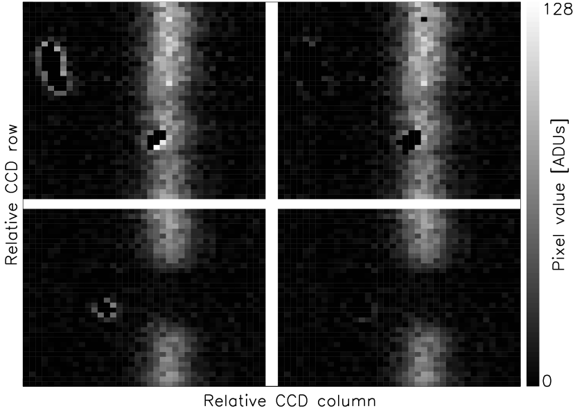
Figure 1: From left to right: Comparison of the original CCD image with cosmics-ray hits and sky line, the cosmic-ray removal of LACosmics (still with sky line), of the REDUCE pipeline (identified pixels affected by cosmic rays set to zero and sky removed), and our new algorithm implemented in the STELLA pipeline (same as for the REDUCE pipeline) for the two parts of the UVES spectrum shown in Fig. 5 which are affected by cosmic-ray hits. LACosmics does not completely remove the cosmic-ray hits and replaces the identified pixels with averages of the surrounding pixels. Both the REDUCE and the STELLA pipelines set the mask value of the identified pixels to zero and remove these pixels from the optimal extraction. While only the cores of the cosmic-ray hits are removed by the REDUCE pipeline, the STELLA pipeline leaves no traces of them.

The STELLA pipeline offers multiple possibilities for removing the scattered light. First of all, standard-IRAF’s apscatter task from the noao.twodspec.apextract package is implemented in the STELLA DRP. Additionally, we re-implemented P&V’s scattered-light subtraction algorithm, as well as the Kriging algorithm (Krige 1951, Matheron 1963). Kriging is very successfully used in Geostatistics for predicting sedimentary rock layers from a small number of bore holes, but is very expensive in terms of computing time. However, clustering the scattered light leads to good results in an acceptable time frame. For the clustering two versions are implemented. The first version assigns the minimum of each rectangular area (cluster) on the CCD (size defined by the user) as scattered-light value to the center of the cluster. This version is very useful if the scattered light needs to be subtracted before the spectral apertures are identified. The second version only looks at areas on the CCD which are not part of a spectral aperture, and assigns the mean value of each cluster (again the sizes of clusters are defined by the user) to the center of each cluster. The complete algorithm will be described in detail in a subsequent paper. Last but not least, setting the wings of the spatial profile (as described in the next paragraphs), can in principle also take care of scattered light, at least if the scattered light is nearly constant underneath a given CCD row.
In addition to the (bug-fixed) optimal-extraction algorithm described by P&V (with and without sky subtraction), the STELLA pipeline also offers two new algorithms for the sky subtraction and the optimal extraction of the object spectrum in the same iterative procedure. In the first version, the initial spatial profile is calculated only from rows which are not affected by sky lines. The second version also sets the wings of the spatial profile to zero, removing sky continuum and (residual) scattered light as well.
Our new algorithms do not involve any re-binning and therefore leave the resulting extracted spectra uncorrelated. Note however that they are still limited to sky lines which are aligned with the rows/columns of the CCD. For the final extraction step, the (oversampled) spatial profile can be cross-correlated to the CCD row in order to find and eliminate offsets between the trace function and the real position of the object spectrum on the CCD. After the cross-correlation for each row, the offsets are fit with a low-order polynomial before being added to the trace function.
All libraries we used for the re-implementation of P&V’s optimal-extraction algorithm are open source and freely available. For reading and writing fits files the cfitsio library has been included. Mathematical procedures use the BLITZ++ library (Veldhuizen & Jernigan, 1997), which provides performance on par with FORTRAN 77/90. The IDL code from P&V was ported as closely as possible to C++. Bugs like possible divisions by zero, which caused the program to crash, were identified and removed in our re-implementation.

2.3 Error estimation and propagation

In the REDUCE pipeline, the actual uncertainties of the individual pixel values are not taken into account at all during the extraction or for the final estimation of the uncertainties. As an error estimate of the final object spectrum P&V calculate

$$\sigma_{\lambda}=\frac{\sum_{x}{(D_{x\lambda}-S_{\lambda}P_{x\lambda})^{2}}}{\sum_{x}P_{x\lambda}-\overline{P_{x\lambda}}},$$ (19)

where $\overline{P_{x\lambda}}$ is the mean value of the spatial profile for the CCD row $\lambda$ ($y$). In our re-implementation of the original algorithm, we calculate the error estimate for the final extracted object spectrum from Eq. 4 and the uncertainties for each pixel in the CCD row:

$$\sigma_{\lambda}^{2}=\frac{\sum_{x}{\sigma_{x\lambda}^{2}F_{x\lambda}^{2}}}{(\sum_{x}{F_{x\lambda}^{2})^{2}}}$$ (20)

where

$$F_{x\lambda}=\sum_{j}P_{x}^{j}W_{x\lambda}^{j}$$ (21)

The new algorithms presented here use the estimated pixel errors, which are given to the program in an additional error image, to calculate the most probable spectrum and background, and propagate the errors through the entire extraction process. This procedure results in much more realistic error estimates for the final object spectra (See Sec. 3). Assuming that flat-fielding and scattered-light subtraction do not introduce additional errors, the uncertainties of the final spectrum and constant background can be calculated as

$$\sigma_{S,\lambda}^{2}=\frac{1}{\Delta_{\lambda}}\sum_{x}{W_{x\lambda}}\mathrm{~{}and}$$ (22)

$$\sigma_{B,\lambda}^{2}=\frac{1}{\Delta_{\lambda}}\sum_{x}{W_{x\lambda}P_{x\lambda}^{2}}$$ (23)

where $\sigma_{S,\lambda}$ and $\sigma_{B,\lambda}$ are the uncertainties for the object spectrum and the background, respectively.

2.4 Data flow chart

If the new programs are invoked by the STELLA pipeline, all parameters for the optimal extraction procedure are stored in one parameterfile. This provides for both an easy overview of the parameters and their values, as well as easy editing. The flow chart for this case is shown in Fig. 2.

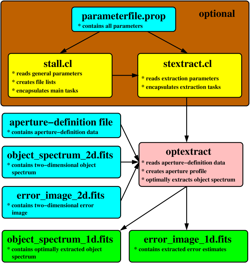
Figure 2: Flow chart of the parameters and data for our new optextract program, if invoked by the STELLA pipeline. The yellow boxes show STELLA tasks, the light blue boxes input files, and the green boxes the output files. Files within the brown box are optional for the execution of the task.

Our new C/C++ programs can be utilised to calculate the scattered light, the normalised Flat, and the instrument profile (quantum efficiency and Blaze function) in the case that a continuous light source over the whole spectral range is available (or the spectrum of the Flat field lamp is known), as well as to remove CCD defects and cosmic-ray hits, and to optimally extract the target data and sky to one-dimensional spectra. As an additional feature, they can create the profile image and the reconstructed object and sky images in 2D, where always possible failures can be easily spotted by comparing them to the original image.

3 Test results

Our new C/C++ modules/classes were tested using the ‘black box’ testing strategy. Testing modules were written to test the different constructors and procedures.
‘Black box’ means that the source code is not known. The tester only knows the interface and checks the results of the procedures due to the possible entry points and variable limits. The testing modules compare the results of the procedures to the expected ones. If a single test goes wrong, the testing module returns immediately.
The comparison with the original IDL pipeline (REDUCE) by P&V could not be done completely, because REDUCE crashed. After fixing a few bugs, the optimal-extraction algorithm was working properly for at least a few spectral orders of ESO/FEROS. As shown in Fig. 3, the resulting profiles are indistinguishable.

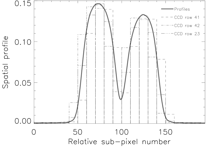
Figure 3: Comparison of the aperture profiles perpendicular to the dispersion axis for ESO/FEROS (with 2-slice image slicer). The thick black line shows the profile calculated with the IDL-REDUCE package from P&V with 10 times oversampling. The over-plotted thin gray line shows the same profile calculated with the STELLA pipeline. Also shown are the histograms of 3 CCD rows in the same aperture: row 41 is a row just before the aperture trace function crosses the border between two CCD columns, row 42 is the row just after that, and row 23 is a row where the trace function goes through the center of the CCD column. All curves/histograms are normalised to an integral of one.

The comparison of the original REDUCE pipeline without sky subtraction to the individual extraction methods performed by the STELLA pipeline (IRAF sum, fit1d, fit2d, and our re-implementation of P&V’s algorithm) is shown in Fig. 4. While the IRAF fit2d algorithm completely fails, the other extraction methods deliver comparable results. Note however that our re-implementation leads to the smoothest object spectrum.

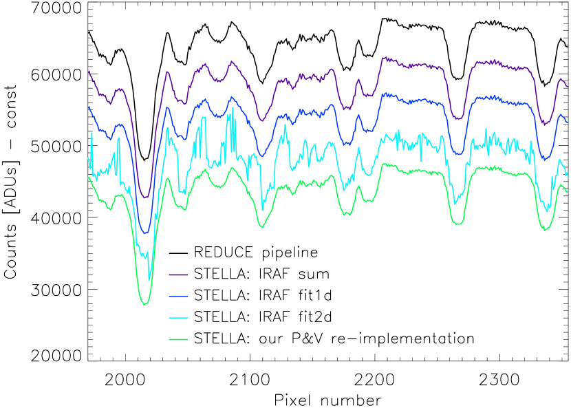
Figure 4: Comparison of the extraction algorithms from the REDUCE and STELLA pipelines for a part of one spectral order (5417–5622 Å) of the variable K0V-star LQ Hya (HD 82558), observed with ESO/FEROS. The lower spectra were shifted downwards for better visibility.

As a test spectrum for the comparison of our new algorithms to the REDUCE pipeline and the UVES pipeline (Ballester et al., 2000) we chose a low-SNR observation of LMC-X1 (a stellar-mass black-hole candidate as revealed by the properties of the surrounding material, Wilms et al. 1998) showing strong sky lines as well as cosmic-ray hits. The spectral region chosen for this test example is $5886.8~{}\mathrm{\AA}<\lambda<5896.5~{}\mathrm{\AA}$ (CCD rows 1363–914 respectively), because it shows 3 sky-emission lines at 5888.192, 5889.959, and 5895.932 Å (CCD rows 1300, 1220, and 940 respectively), 2 stellar absorption lines at $5890.30~{}\mathrm{\AA}$ and $5894.98~{}\mathrm{\AA}$ (CCD rows 288 and 72), and 3 cosmic-ray hits, one in the middle of the spatial profile, one in the wings of an absorption line, and one in a sky line. The mean value of the SNR in this region is approximately 20, making this a low-SNR spectrum where the optimal-extraction algorithm of the UVES pipeline should perform at its best. Fig. 5 shows the original CCD section after bias subtraction, flat-fielding, and scattered-light subtraction as well as a comparison of the spatial profiles calculated with our new optimal sky- and object-extraction algorithms to the algorithm by P&V.

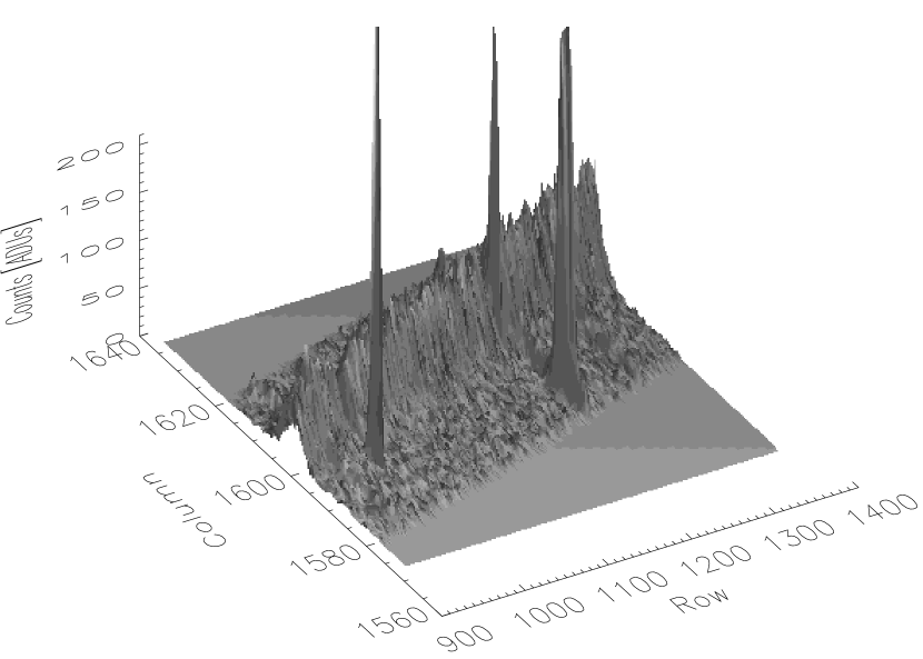
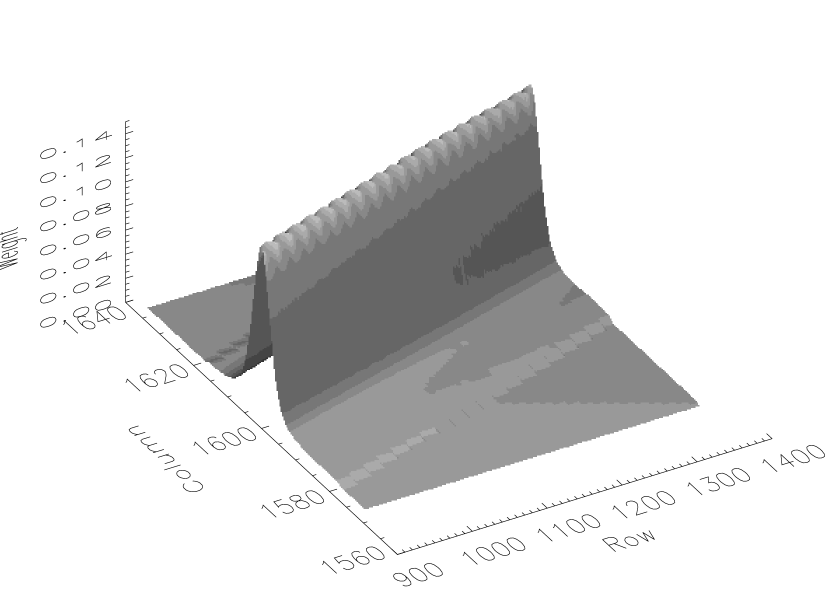
a) b) c)

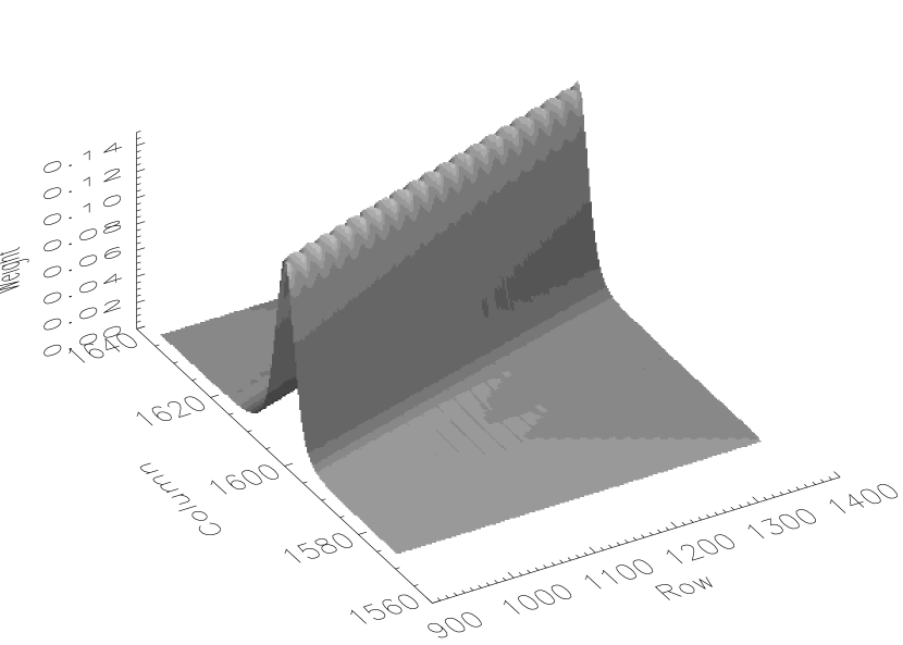
Figure 5: Part of a spectral order of LMC-X1 in the red, observed with UVES, showing strong sky lines as well as cosmic-ray hits. The spectral region chosen for this test example is $5886.8~{}\mathrm{\AA}<\lambda<5896.5~{}\mathrm{\AA}$ (CCD rows 1363–914 respectively), because it shows 3 sky-emission lines at 5888.192, 5889.959, and 5895.932 Å (CCD rows 1300, 1220, 940 respectively), 2 stellar absorption lines at $5890.30~{}\mathrm{\AA}$ and $5894.98~{}\mathrm{\AA}$ (CCD rows 288 and 72), and 3 cosmic-ray hits, one in the middle of the spatial profile, one in the wings of an absorption line, and one in a sky line: a) Original image after bias subtraction, flat-fielding, and scattered-light subtraction. b) Spatial profile calculated with our re-implementation of the original algorithm by P&V. c) Spatial profile calculated with our new algorithm. Note that the wings of the profile shown in b) show small steps at the limits of the extraction width, which disappeared in c). The ripples visible at the top of the profiles are caused by the trace function crossing columns of the CCD.

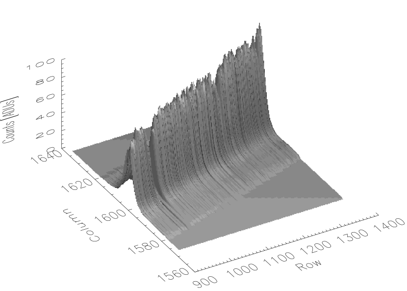
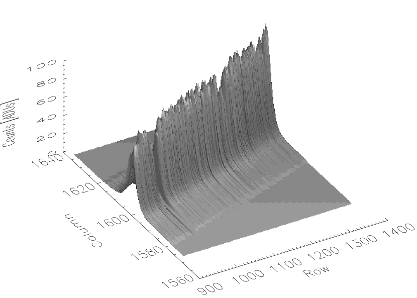
a) b) c)

Figure 6: Comparison of the reconstructed object spectra from Fig. 5. a) Original version by P&V without proper cosmic-ray removal at row 1206. While the spike at the wing of the spatial profile is properly removed, the cosmic ray close to the profile center causes a spike in an absorption line in the extracted object spectrum, which partially fills in the absorption feature. b) Our re-implementation, all cosmic-ray hits properly removed. c) Our new algorithm with all spikes removed and the wings of the spatial profile going down to zero as they should.

In Fig. 6 we compare the reconstructed object spectra from the original version by P&V (a), our re-implementation (b), and our new algorithm (c). While the cosmic-ray hit near the center of the spatial profile causes a spike at row 1206 in the extracted object spectrum shown in a), the cosmic rays are properly removed by our algorithms shown in (b) and (c). The main difference between b) and c) is that in c) the profile goes down to zero at the wings (as one would expect for a point source), while in b) too much weight is given to the background.

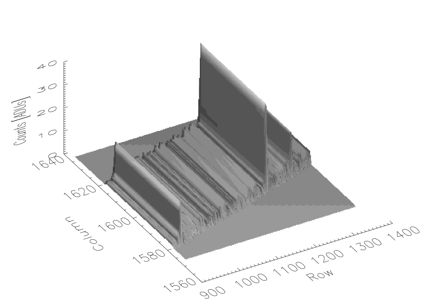
a) b) c)

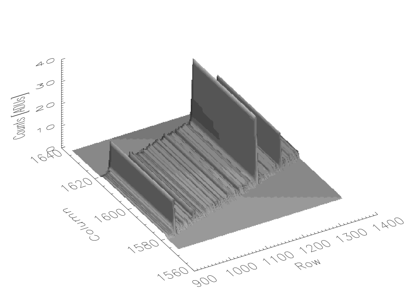
Figure 7: Comparison of the reconstructed sky spectra from Fig. 5. Visible are three sky lines at rows 940 (5895.932 Å), 1220 (5889.959 Å), and 1300 (5888.192 Å). The sky images are scaled the same and the surrounding pixels are set to zero for a better visiblity of the sky. a) Original version by P&V – as expected nearly identical to b) (our re-implementation). The sky line at row 1220 is slightly overestimated. c) Our new algorithm with the smoothest sky and all sky lines properly reproduced (as shown below). Even an additional sky line at row 982 (5894.472 Å) clearly shows up which completely vanishes in the noise of the other reconstructed sky spectra.

The comparison of the reconstructed sky spectra in the cases of (a), (b), and (c) is shown in Fig. 7. We have three sky lines visible at rows 940 (5895.932 Å), 1220 (5889.959 Å), and 1300 (5888.192 Å). In (a) the sky is relatively noisy and the strongest line is 13% higher than in our (c) method. As expected, our re-implementation of the original algorithm leads to nearly identical results (b). Our new optimal extraction and sky-subtraction algorithm (c) leads to the smoothest sky results. All sky lines are properly reproduced, as shown below. Using our new algorithm we additionally find a new sky line at row 982. This line can only be inferred in the other sky spectra. A comparison to the catalogue of optical sky emission from UVES (Hanuschik 2003) identifies it as the 5894.472 Å line.

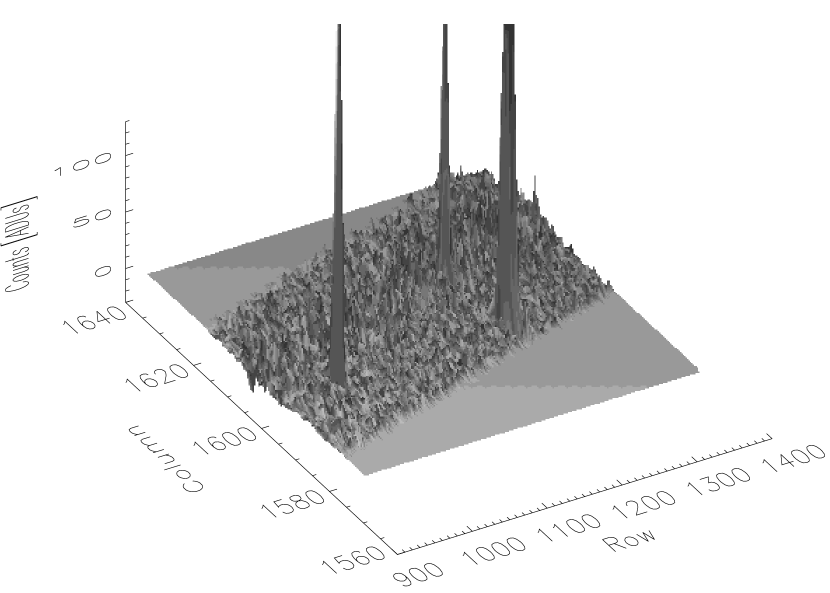
a) b) c)

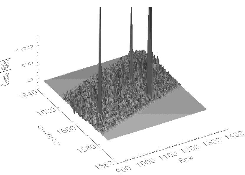
Figure 8: Comparison of the differences between the CCD image from Fig. 5 and the reconstructed object and sky spectra from Fig.s 6 and 7. No obvious remaining structures which would indicate systematic discrepancies between the CCD image and the reconstruction can be seen.

The differences between the CCD image shown in Fig. 5 and the reconstructed object and sky spectra from Fig.s 6 and 7 are shown in Fig. 8. No remaining structures which would indicate systematic discrepancies between the CCD image and the reconstruction are obvious in any of the images.

The comparison of the resulting sky and object spectra from the original implementation by P&V to our re-implementation, our new algorithms, as well as to the UVES pipeline, is presented in Fig. 9. Shown are the optimally extracted object spectra, the sky spectra, and the estimated SNRs. The UVES pipeline uses a similar approach as we present here, but always assumes a Gaussian for the spatial profile, leading to systematic errors. The sky is calculated by fitting the Gaussian profile plus constant (sky) to the CCD row. Again, assuming a Gaussian for the spatial profile is leading to systematic errors in the sky as well. As it can be seen in the figure, our new algorithms are leading to the smoothest sky and the least sky- and cosmic-ray residuals in the object spectrum. As expected, the sky values calculated with the REDUCE pipeline and our re-implementation are nearly identical. Note however that the REDUCE pipeline, as well as the UVES pipeline, produce a spike at $5890.29~{}\mathrm{\AA}$ caused by a residual cosmic-ray hit. The SNR calculated by the REDUCE pipeline is unrealistic (we still cannot reproduce Eq. 19). In contrast, our error estimates (Eq. 20 for our re-implementation and Eq.s 22 and 23 for our new algorithms), using the propagated uncertainties for every pixel, are similar to the error estimates stated by the UVES pipeline. However, as we could not find a documentation on the algorithm used to calculate the UVES uncertainties, we cannot comment on the stated UVES SNR too much. As the object extraction and sky subtraction are done in a way very similar to our new algorithms, we can assume that the errors are also calculated in a similar way. Given that the spatial profile is close to a Gaussian, this explains why the SNR stated by the UVES pipeline is very close to the SNR for our new algorithms. Note however that the UVES object spectrum was rebinned using an oversampling factor of $\sim 1.5$. While oversampling preserves the resolution, it smooths the spectrum, making it appear as if it had a higher SNR. Visibly, our new extraction method leads to an object spectrum even smoother than the rebinned spectrum produced by the UVES pipeline. Compared to the SNR for the original algorithm by P&V, calculated from the propagated pixel uncertainties, our new algorithms lead to a SNR $\approx 15-20$ % higher. The simple-sum extraction (which is not shown in the plot because of the sky lines and cosmic-ray hits) leads to a calculated SNR of only $\approx 3.5$, even with an aperture width only slightly larger than the object spectrum!

Figure 9: Plot comparing the resulting object and sky spectra of the spectral region shown in Fig. 5, extracted with the original sky-subtraction algorithm from P&V, our new programs, and the UVES pipeline. The upper part of the image shows the extracted object spectra, the middle part shows the extracted sky, and the lower part shows the estimated SNR. In the upper two parts the spectra were shifted upwards for better visibility. Note the spike at $5890.29~{}\mathrm{\AA}$ in the UVES spectrum and the original implementation by P&V, which is caused by a cosmic-ray hit.

In Fig.s 10 and 11 a comparison of the performance of the original sky-subtraction algorithm by P&V to our new programs is shown for the case that the object is close to the slit edge. The images show a short part of a spectrum of LMC-X1, taken with UVES in the blue arm. While the original sky-subtraction algorithm by P&V is struggling to remove the background properly, our new algorithm performs much better, resulting in a $\approx 50\%$ gain for the SNR of the object spectrum. Note that the spectrum actually shows an accretion disk surrounding the black hole and not a sky emission line.

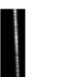
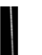
Figure 10: Plot comparing the resulting sky (actually accretion disk) and object spectra for a short part of an UVES spectrum of LMC-X1 in the blue arm, extracted with our re-implementation of the original sky-subtraction algorithm from P&V and our new programs. The most left image is the bias and scattered-light subtracted and flat-fielded CCD image, followed by the reconstructed sky (original algorithm and our new programs), CCD minus reconstructed sky, reconstructed object image, and CCD minus reconstructed object. As the object is close to the slit edge, the original algorithm by P&V is struggling to remove the sky properly, while our new programs deliver a much better result. Note that the apparent over subtraction of the sky in the middle panel is not real and only due to the fact that the right aperture limit is outside the slit’s image where there is no signal.

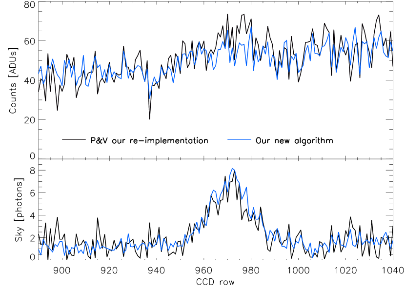
Figure 11: Plot of the object and sky spectra shown in Fig. 10. The SNR measured with IRAF splot is 6.3 for the original algorithm by P&V and 9.1 for our new algorithms – an improvement of nearly 50%.

Shown in Fig. 12 is the computing time of our new programs and the original REDUCE procedures for one spectral order of the ESO/FEROS spectrograph (18x4089 pixels). It shows that our C/C++ re-implementation is about 10 times faster than the IDL version. In times of major spectroscopic surveys with multi-object spectrographs, this is a major advantage over the original programs.

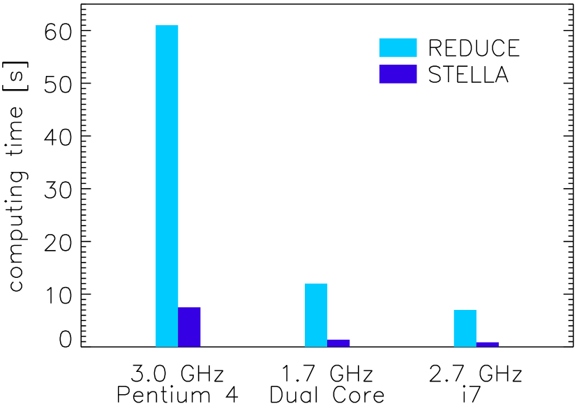
Figure 12: Plot comparing the computing time for the calculation of the aperture profile and optimal extraction of one order (15x4089 pixels) for the ESO/FEROS spectrograph. Our C/C++ re-implementation of P&V’s algorithms is about 10 times faster than the original IDL procedures, making it perfectly suitable for large spectroscopic surveys.

Our new programs have been extensively tested with a wide range of spectrographs, including slits and fibre feeds, prisms and gratings, Echelle spectra, multi-object spectra, and IFUs. Comparisons of the STELLA pipeline to the results of the pipelines provided by the individual observatories and to standard IRAF have shown that our pipeline can lead to significant SNR improvements. The UVES pipeline has been optimised for low SNRs and always assumes a Gaussian profile perpendicular to the dispersion axis for the optimal-extraction algorithm. For low SNR the random error of the Poisson noise (photon noise) is larger than the systematic error introduced by this approximation. In the low-SNR regime, assuming a Gaussian spatial profile is therefore an acceptable approximation. However, profile determination is the most critical step for variance weighted (optimal) extraction. Assuming an incorrect spatial profile can lead to large systematic errors for high-SNR data. These systematics drop the achievable SNR significantly and can introduce ripples in the extracted spectra, both leading to larger uncertainties in the stellar parameters derived from these spectra.
The optimal-extraction algorithms of standard IRAF are also known to have room for improvement. The simple sum nearly always leads to a higher SNR than these ‘optimal extraction’ algorithms, even if apsum is fed with the most probable profile calculated with P&V’s profile-fitting algorithm. Our new algorithms are now allowing for the utilisation of a state-of-the-art optimal-extraction algorithm within the IRAF environment, as well as most other existing data-reduction packages.

4 Conclusions

The presented new implementation of the state-of-the-art optimal-extraction algorithm developed by P&V can now easily be integrated in IRAF and most other existing data-reduction packages and programming languages. It allows for scattered-light subtraction, profile calculation, error propagation, and optimal extraction of Coudé and Echelle slit spectra as well as fibre feeds. For slit spectra a new optimal sky ex-/subtraction algorithm at the Poisson limit was developed, which works even for extended objects, short slits, or if the observed star is at the slit’s end. Our progams offer the new optimal extraction and sky-subtraction algorithms as well as the original ones by P&V. The re-implementation in C++ is about 10 times faster than the original one, making it perfectly suitable for large surveys. Our new programs have been extensively bug fixed and successfully tested with spectra from VLT/UVES, ESO/CES, ESO/FEROS, NTT/EMMI, NOT/ALFOSC, STELLA/SES, SSO/WiFeS, and, finally P60/SEDM-IFU. As already shown by P&V, their optimal-extraction algorithm can lead to a significant improvement in the SNR compared to standard IRAF and other DRPs. In this paper we have shown that using our improved algorithms for cosmic-ray/CCD-defect removal and background subtraction we can again achieve a SNR gain of 15-50% compared to the original algorithms by P&V. This is leading to much smaller errors in parameter estimates calculated from our optimally extracted spectra compared to other DRPs.

5 Acknowledgements

We would like to thank the anonymous referee for the helpful comments, which significantly increased the scientific content of this paper, and Heidi Viets and Andrew Fathy for proof reading the manuscript. Funding for the project has been provided by the Taiwanese National Science Council (grant numbers NSC 101-2112-M-008-017-MY3 and NSC 101-2119-M-008-007-MY3).

References

- Ballester et al. (2000) P. Ballester, A. Modigliani, O. Boitquin, S. Cristiani, R. Hanuschik, A. Kaufer, S. Wolf: 2000, ESO Messenger 101, 31
- Ben-Ami et al. (2012) S. Ben-Ami, N. Konidaris, R. Quimby, J. T. C. Davis, C. C. Ngeow, A. Ritter, A. Rudy: 2012, SPIE Conference Series 8446, 316
- Bevington & Robinson (2003) P. R. Bevington and D. K. Robinson: Data reduction and error analysis for the physical sciences: 2003, McGraw-Hill, 98
- Bolton & Schlegel (2010) A. S. Bolton and D. J. Schlegel: 2010, PASP 122, 248
- Dekker et al. (1986) H. Dekker, B. Delabre, and S. D’Odorico: SPIE 627, 39
- Dekker et al. (2000) H. Dekker, S. D’Odorico, A. Kaufer, B. Delabre and H. Kotzlowski: SPIE Conference Series 4008, 534
- Dopita et al. (2010) M. Dopita, J. Rhee, C. Farage, P. McGregor, G. Bloxham, A. Green, B. Roberts, J. Neilson, G. Wilson, P. Young, P. Firth, G. Busarello, P. Merluzzi: 2010, AP&SS 327, 245
- Enard (1982) D. Enard: 1982, SPIE Conference Series 331, 232
- Hall et al. (1994) Jeffrey C. Hall, Eliza E. Fulton, David P. Huenemoerder, Alan D. Welty and James E. Neff: 1994, PASP 106, 315
- Glazebrook & Bland-Hawthorn (2001) K. Glazebrook and J. Bland-Hawthorn: 2001, PASP 113, 197
- Hanuschik (2003) R. Hanuschik: 2003, A&A 407, 1157
- Horne (1986) Keith Horne: 1986, PASP 98, 609
- Kaufer et al. (1999) A. Kaufer, O. Stahl, S. Tubbesing, P. Nørregaard, G. Avila, P. Francois, L. Pasquini, A. Pizzella: 1999, The Messenger 95, 8
- Kinney et al. (1991) A. L. Kinney, R. C. Bohlin and J. D. Neill: 1991, PASP 103, 694
- Krige (1951) Krige D.G, 1951, Master’s thesis, University of Witwatersrand
- Marsh (1989) T. R. Marsh: 1989, PASP 101, 1032
- Matheron (1963) G. Matheron: 1963, Economic Geology, 58, 1246–1266
- Mukai (1990) K. Mukai: 1990, PASP 102, 183
- Piskunov & Valenti (2002) N. E. Piskunov and J. A. Valenti: 2002, A&A 385, 1095
- Ritter & Washüttl (2004) A. Ritter and A. Washüttl: 2004, Astronomische Nachrichten 325, 663
- Robertson (1986) J. G. Robertson: 1986, PASP 98, 1220
- Sembach & Tonry (1996) K. R. Sembach and J. L. Tonry: 1996, AJ 112, 797
- Sharp & Birchall (2010) R. Sharp and M. N. Birchall: 2010, PASA 27, 91
- Smith et al. (2004) G. A. Smith, W. Saunders, T. Bridges, V. Churilov, A. Lankshear, J. Dawson, D. Correll, L. Waller, R. Haynes, and G. Frost: 2004, SPIE Vonference Series 5492, 410
- Strassmeier et al. (2001) K. G. Strassmeier, T. Granzer, M. Weber, M. Woche, G. Hildebrandt, S.-M. Bauer, J. Paschke, M. M. Roth, A. Washuettl, K. Arlt, P. A. Stolz, J. H. M. M. Schmitt, A. Hempelmann, H.-J. Hagen, H. Ruder, P. L. Palle, R. Arnay: 2001, Astronomische Nachrichten 322, 287
- Tody (1986) Doug Tody: 1986, SPIE Instrumentation in Astronomy VI 627, 733
- Valdes (1992) F. Valdes: 1992, Astronomical Data Analysis Software and Systems I, ASP Conf. Ser. 25, 398
- van Dokkum (2001) P. G. van Dokkum: 2001, PASP 113, 1420
- Veldhuizen & Jernigan (1997) T. L. Veldhuizen and M. E. Jernigan: 1997, Proceedings of the 1st International Scientific Computing in Object-Oriented Parallel Environments (ISCOPE’97), Lecture Notes in Computer Science
- Vershueren & Hensberge (1990) W. Vershueren and H. Hensberge: 1990, A&A 240, 216
- Wilms et al. (1998) J. Wilms, M. A. Nowak, J. B. Dove, K. Pottschmidt, W. A. Heindl, M. C. Begelman, R. Staubert: 1998, STIN 99, 70941