{textblock*}100pt(316pt,-154pt) CERN-PH-TH/2013-261 Euclidean Dynamical Triangulation revisited:
is the phase transition really first order?


Institute for Theoretical Physics, ETH Zürich, CH - 8093 Zürich, Switzerland
E-mail
   Philippe de Forcrand
Institute for Theoretical Physics, ETH Zürich, CH - 8093 Zürich, Switzerland and
CERN, Physics Department, TH Unit, CH-1211 Genève 23, Switzerland
E-mail
forcrand@itp.phys.ethz.ch
Abstract:

The transition between the two phases of 4D Euclidean Dynamical Triangulation [1] was long believed to be of second order until in 1996 first order behavior was found for sufficiently large systems [3, 4]. However, one may wonder if this finding was affected by the numerical methods used: to control volume fluctuations, in both studies [3, 4] an artificial harmonic potential was added to the action; in [4] measurements were taken after a fixed number of accepted instead of attempted moves which introduces an additional error. Finally the simulations suffer from strong critical slowing down which may have been underestimated.
In the present work, we address the above weaknesses: we allow the volume to fluctuate freely within a fixed interval; we take measurements after a fixed number of attempted moves; and we overcome critical slowing down by using an optimized parallel tempering algorithm [6]. With these improved methods, on systems of size up to N4=64subscript𝑁464N_{4}=64k 4-simplices, we confirm that the phase transition is first order.

1 Introduction

The transition between the two phases of 4D Euclidean Dynamical Triangulation (EDT)[1] was first believed to be of 2ndordersuperscript2ndorder2^{\text{nd}}\,\text{order} until 1996 where in [3] for the first time 1stordersuperscript1storder1^{\text{st}}\,\text{order} behavior was reported for a system consisting of N4=32subscript𝑁432N_{4}=32k 4-simplices. Shortly afterwards this finding was verified in [4] and extended to larger systems with N4=64subscript𝑁464N_{4}=64k. However, we were not completely convinced by the numerical methods used in the latter work; there were three things which disturbed us:

  1. 1.

    Measurements were taken after a fixed number of accepted (instead of attempted) moves, which introduces a systematic error.

  2. 2.

    The use of an artificial harmonic potential to control volume fluctuations also introduces a systematic error.

  3. 3.

    Autocorrelation and thermalization time could easily have been underestimated.

Therefore we wanted to crosscheck these old results with our own, hopefully correct code which satisfies detailed balance, uses a potential well instead of a harmonic potential to control volume fluctuations, and makes use of parallel tempering to cope with critical slowing down.

1.1 The EDT Model

In 4-dimensional Euclidean Dynamical Triangulation (EDT)[1] the formal path integral for Euclidean (local SO(4)SO4\operatorname{SO}\left(4\right) instead of SO(3,1)SO31\operatorname{SO}\left(3,1\right) symmetry) gravity,

Z=𝒟[g\indices]μνeSEH[g\indices]μν,Z\,=\,\int\mathcal{D}\left[g\indices{{}_{\mu}{}_{\nu}}\right]\operatorname{e}^{-\,S_{EH}\mathop{\left[g\indices{{}_{\mu}{}_{\nu}}\right]}}, (1)

with SEH=116πGd4xg(R2Λ)subscript𝑆𝐸𝐻116𝜋𝐺superscriptd4𝑥𝑔𝑅2ΛS_{EH}=-\frac{1}{16\pi G}\,\int\mathrm{d}^{4}\,x\sqrt{g}\mathop{\left(R-2\Lambda\right)} being the Einstein-Hilbert action, is regularized by approximating the configuration space (space of all diffeomorphism inequivalent 4-metrics) with the space of simplicial piecewise linear (PL) manifolds consisting of equilateral 4-simplices with fixed edge length a𝑎a (such manifolds are also called abstract triangulations). Under such a discretization, the Einstein-Hilbert action turns into the Einstein-Regge action which for equilateral 4-simplices and a space-time of topology S4superscriptS4\operatorname{S}^{4} takes the simple form SER=κ2N2+κ4N4subscript𝑆𝐸𝑅subscript𝜅2subscript𝑁2subscript𝜅4subscript𝑁4S_{ER}=-\kappa_{2}N_{2}+\kappa_{4}N_{4}, where the Nisubscript𝑁𝑖N_{i} label the number of i𝑖i-simplices in the PL manifold, κ2=V24Gsubscript𝜅2subscript𝑉24𝐺\kappa_{2}=\frac{V_{2}}{4\,G} and κ4=10arccos(1/4)V2+ΛV48πGsubscript𝜅410arccos14subscript𝑉2Λsubscript𝑉48𝜋𝐺\kappa_{4}=\frac{10\operatorname{arccos}\mathop{\left(1/4\right)}V_{2}+\Lambda V_{4}}{8\pi G}, with Vn=ann+1n!2nsubscript𝑉𝑛superscript𝑎𝑛𝑛1𝑛superscript2𝑛V_{n}=a^{n}\frac{\sqrt{n+1}}{n!\sqrt{2^{n}}} being the volume of a n𝑛n-simplex and G𝐺G, ΛΛ\Lambda the gravitational and cosmological coupling respectively. The partition function (1) can now be written as

Z(κ2,κ4)=T1CTeκ2N2(T)κ4N4(T)=N4Z(κ2,N4)eκ4N4,𝑍subscript𝜅2subscript𝜅4subscript𝑇1subscript𝐶𝑇superscriptesubscript𝜅2subscript𝑁2𝑇subscript𝜅4subscript𝑁4𝑇subscriptsubscript𝑁4𝑍subscript𝜅2subscript𝑁4superscriptesubscript𝜅4subscript𝑁4Z\mathop{\left(\kappa_{2},\kappa_{4}\right)}\,=\,\sum\limits_{T}\,\frac{1}{C_{T}}\,\operatorname{e}^{\kappa_{2}\,N_{2}\mathop{\left(T\right)}\,-\,\kappa_{4}\,N_{4}\mathop{\left(T\right)}}\,=\,\sum\limits_{N_{4}}\,Z\mathop{\left(\kappa_{2},N_{4}\right)}\,\operatorname{e}^{-\kappa_{4}\,N_{4}}, (2)

where the sum after the first equality sign runs over all abstract triangulations T𝑇T of S4superscriptS4\operatorname{S}^{4} and CTsubscript𝐶𝑇C_{T} is for each T𝑇T a corresponding symmetry factor111CTsubscript𝐶𝑇C_{T} is assumed to be  1similar-toabsent1\sim\,1 for sufficiently large systems.. The second equality sign defines the canonical partition function Z(κ2,N4)𝑍subscript𝜅2subscript𝑁4Z\mathop{\left(\kappa_{2},N_{4}\right)}. The partition function (2) is suitable for use in a Markov chain Monte Carlo simulation with Metropolis updates consisting of the so-called Pachner moves [1].

1.2 Phase Diagram

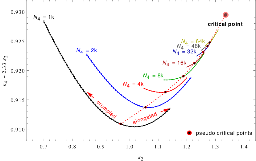
The grand canonical partition function (2) is finite only if κ4>κ4cr(κ2)subscript𝜅4superscriptsubscript𝜅4𝑐𝑟subscript𝜅2\kappa_{4}>\kappa_{4}^{cr}\mathop{\left(\kappa_{2}\right)}. We therefore have a critical line for convergence in the (κ2,κ4)subscript𝜅2subscript𝜅4\mathop{\left(\kappa_{2},\kappa_{4}\right)}-plane, given by κ4cr(κ2)superscriptsubscript𝜅4𝑐𝑟subscript𝜅2\kappa_{4}^{cr}\mathop{\left(\kappa_{2}\right)}. To obtain the thermodynamic limit (N4)subscript𝑁4\mathop{\left(N_{4}\rightarrow\infty\right)} we have to ensure that κ4N4κ4cr(κ2)subscript𝜅4subscript𝑁4superscriptsubscript𝜅4𝑐𝑟subscript𝜅2\kappa_{4}\overset{\scriptscriptstyle N_{4}\rightarrow\infty}{\longrightarrow}\kappa_{4}^{cr}\mathop{\left(\kappa_{2}\right)}. For quasi-canonical simulations around some fixed volume N¯4subscript¯𝑁4\bar{N}_{4}, it follows from (2) that we can define a pseudo-critical κ4pcr(κ2,N¯4)=ln(Z(κ2,N4))N4|N4=N¯4superscriptsubscript𝜅4𝑝𝑐𝑟subscript𝜅2subscript¯𝑁4evaluated-at𝑍subscript𝜅2subscript𝑁4subscript𝑁4subscript𝑁4subscript¯𝑁4\kappa_{4}^{pcr}\mathop{\left(\kappa_{2},\bar{N}_{4}\right)}=\frac{\partial\ln\mathop{\left(Z\mathop{\left(\kappa_{2},N_{4}\right)}\right)}}{\partial N_{4}}\big{|}_{\scriptscriptstyle N_{4}=\bar{\scriptscriptstyle N}_{4}}, which corresponds to the value of κ4subscript𝜅4\kappa_{4} for which the N4subscript𝑁4N_{4}-distribution is flat around N¯4subscript¯𝑁4\bar{N}_{4}.

Refer to caption
Figure 1: Phase diagram for 4D EDT. The Figure shows κ4pcr(κ2,N4)superscriptsubscript𝜅4𝑝𝑐𝑟subscript𝜅2subscript𝑁4\kappa_{4}^{pcr}\mathop{\left(\kappa_{2},N_{4}\right)} as a function of κ2subscript𝜅2\kappa_{2} for different N4subscript𝑁4N_{4} together with the corresponding pseudo-critical points (κ2pcr(N4),κ4pcr(κ2pcr(N4),N4))superscriptsubscript𝜅2𝑝𝑐𝑟subscript𝑁4superscriptsubscript𝜅4𝑝𝑐𝑟superscriptsubscript𝜅2𝑝𝑐𝑟subscript𝑁4subscript𝑁4\mathop{\left(\kappa_{2}^{pcr}\mathop{\left(N_{4}\right)},\kappa_{4}^{pcr}\mathop{\left(\kappa_{2}^{pcr}\mathop{\left(N_{4}\right)},N_{4}\right)}\right)}. The dotted red line separates the crumpled from the elongated phase; in the limit N4subscript𝑁4N_{4}\,\rightarrow\,\infty this line ends at the critical point: (κ2cr,κ4cr)superscriptsubscript𝜅2𝑐𝑟superscriptsubscript𝜅4𝑐𝑟\mathop{\left(\kappa_{2}^{cr},\kappa_{4}^{cr}\right)}. To improve readability, the y-axis shows (κ42.33κ2)subscript𝜅42.33subscript𝜅2\mathop{\left(\kappa_{4}-2.33\,\kappa_{2}\right)} instead of κ4subscript𝜅4\kappa_{4} itself.
Refer to caption
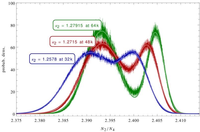
Figure 2: N2subscript𝑁2N_{2}-distribution for systems of size N4=subscript𝑁4absentN_{4}\,=\, 32k (blue), 48k (red) and 64k (green): the solid lines are double-Gaussian fits to the data. It can be seen that the double peak structure becomes more pronounced with increasing system size and there is no sign that the peaks will merge again in the thermodynamic limit. This is characteristic of a 1stordersuperscript1storder1^{\text{st}}\,\text{order} transition.
Refer to caption
Refer to caption
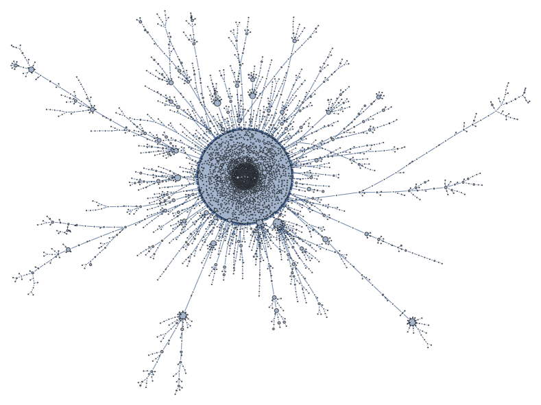
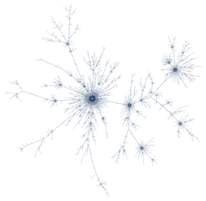
Figure 3: Representative configurations in the crumpled (left, κ2=1.24subscript𝜅21.24\kappa_{2}=1.24) and elongated (right, κ2=1.27subscript𝜅21.27\kappa_{2}=1.27) phase at system size N432subscript𝑁432N_{4}\approx 32k: in the crumpled phase, the triangulation consists of one large, highly connected bunch with outgrowths which are at least an order of magnitude smaller. In the elongated phase on the other hand, although a largest component still exists and may be called “mother universe”, it is much smaller than in the crumpled phase and some of its outgrowths (the “babies”) are of comparable size.

For constant N4subscript𝑁4N_{4}, we can define (see Fig. 2) a line κ4pcr(κ2,N4)superscriptsubscript𝜅4𝑝𝑐𝑟subscript𝜅2subscript𝑁4\kappa_{4}^{pcr}\mathop{\left(\kappa_{2},N_{4}\right)} as a function of κ2subscript𝜅2\kappa_{2}, along which two phases are separated by a pseudo-critical point at κ2=κ2pcr(N4)subscript𝜅2superscriptsubscript𝜅2𝑝𝑐𝑟subscript𝑁4\kappa_{2}=\kappa_{2}^{pcr}\mathop{\left(N_{4}\right)}. For κ2<κ2pcr(N4)subscript𝜅2superscriptsubscript𝜅2𝑝𝑐𝑟subscript𝑁4\kappa_{2}<\kappa_{2}^{pcr}\mathop{\left(N_{4}\right)} we are in the crumpled phase where a typical configuration is highly collapsed in the sense that the distance between any two 4-simplices is very short, leading to a large (infinite) Hausdorff dimension. For κ2>κ2pcr(N4)subscript𝜅2superscriptsubscript𝜅2𝑝𝑐𝑟subscript𝑁4\kappa_{2}>\kappa_{2}^{pcr}\mathop{\left(N_{4}\right)} we are in the elongated phase with Hausdorff dimension  2similar-toabsent2\sim\,2, where a typical configuration consists of a so-called baby-universe tree: the total volume is subdivided into smaller parts, the baby-universes, which are pairwise connected by only a small neck. This structure is hierarchical in a treelike manner: consider the largest baby-universe as “mother” with outgrowing smaller “babies” which in turn give birth to their own “babies”, and so on (see Fig. 3).
The true critical point in the thermodynamic limit is obtained as

(κ2cr,κ4cr)=limN4(κ2pcr(N4),κ4pcr(κ2pcr(N4),N4)).superscriptsubscript𝜅2𝑐𝑟superscriptsubscript𝜅4𝑐𝑟subscriptsubscript𝑁4superscriptsubscript𝜅2𝑝𝑐𝑟subscript𝑁4superscriptsubscript𝜅4𝑝𝑐𝑟superscriptsubscript𝜅2𝑝𝑐𝑟subscript𝑁4subscript𝑁4\mathop{\left(\kappa_{2}^{cr},\kappa_{4}^{cr}\right)}\,=\,\lim\limits_{N_{4}\rightarrow\infty}\,\mathop{\left(\kappa_{2}^{pcr}\mathop{\left(N_{4}\right)},\kappa_{4}^{pcr}\mathop{\left(\kappa_{2}^{pcr}\mathop{\left(N_{4}\right)},N_{4}\right)}\right)}. (3)

2 Simulation Methods

We are interested in the canonical system, but as there is no set of ergodic moves known for the space of triangulations of fixed volume, we can only run quasi-canonical222I.e. grand canonical simulations where the volume is constrained to fluctuate around some desired volume N¯4subscript¯𝑁4\bar{N}_{4}. Markov chain Monte Carlo simulations with local updates consisting of the five Pachner moves.

2.1 Detailed Balance

Calling Tksubscript𝑇𝑘T_{k} the current triangulation in our Markov chain, we obtain Tk+1subscript𝑇𝑘1T_{k+1} as follows:

  1. 1.

    randomly choose a move type n{0,,4}𝑛04n\in\mathop{\left\{0,\ldots,4\right\}}

  2. 2.

    randomly choose one of the N4subscript𝑁4N_{4} 444-simplices of Tksubscript𝑇𝑘T_{k} and call it D𝐷D

  3. 3.

    randomly choose one of the (5n+1)binomial5𝑛1\binom{5}{n+1} n𝑛n-simplices contained in D𝐷D and call it S𝑆S

  4. 4.

    perform a Metropolis test with acceptance probability pn(Tk,S)subscript𝑝𝑛subscript𝑇𝑘𝑆p_{n}\mathop{\left(T_{k},S\right)}:

    • accept: Tk+1subscript𝑇𝑘1T_{k+1} is obtained from Tksubscript𝑇𝑘T_{k} by applying the n𝑛n-move at S𝑆S

    • reject: Tk+1=Tksubscript𝑇𝑘1subscript𝑇𝑘T_{k+1}=T_{k}

The acceptance probability at step 4 is given by [5]

pn(T,S)={pn(N4(T))ifn-move possible at ST0else,subscript𝑝𝑛𝑇𝑆casessubscript𝑝𝑛subscript𝑁4𝑇ifn-move possible at ST0elsep_{n}\mathop{\left(T,S\right)}=\begin{cases}p_{n}\mathop{\left(N_{4}\mathop{\left(T\right)}\right)}\quad&\text{\small if}\quad\text{\small$n$-move possible at $S\,\in\,T$}\\ 0\quad&\text{\small else}\end{cases}, (4)

where pn(N4)=min{1,N4N4+ΔN4(n)eκ2ΔN2(n)κ4ΔN4(n)}subscript𝑝𝑛subscript𝑁41subscript𝑁4subscript𝑁4Δsubscript𝑁4𝑛superscriptesubscript𝜅2Δsubscript𝑁2𝑛subscript𝜅4Δsubscript𝑁4𝑛p_{n}\mathop{\left(N_{4}\right)}=\textstyle\min\mathop{\left\{1,\frac{\scriptstyle N_{4}}{\scriptstyle N_{4}+\Delta N_{4}\mathop{\left(n\right)}}\,\operatorname{e}^{\kappa_{2}\Delta N_{2}\mathop{\left(n\right)}-\kappa_{4}\Delta N_{4}\mathop{\left(n\right)}}\right\}} is the so-called reduced transition probability, ΔNi(n)Δsubscript𝑁𝑖𝑛\Delta N_{i}\mathop{\left(n\right)} labels the change of Nisubscript𝑁𝑖N_{i} under a n𝑛n-move, and a n𝑛n-move is considered as possible at S𝑆S if S𝑆S is contained in (5n)5𝑛\mathop{\left(5-n\right)} 444-simplices333If a n𝑛n-simplex is contained in (5n)5𝑛\mathop{\left(5-n\right)} 4-simplices, the complex spanned by these 4-simplices can be replaced by another complex which has the same boundary but consists of (n+1)𝑛1\mathop{\left(n+1\right)} 4-simplices which share a common (dn)𝑑𝑛\mathop{\left(d-n\right)}-simplex (orthogonal/dual to the initial n𝑛n-simplex). This is precisely the action of a Pachner n𝑛n-move. and the application of the move does not violate the manifold constraint which requires that the move will not produce any simplex which already exists in the triangulation.

2.2 Controlling the Volume

In previous work [1, 3, 4], the volume was controlled by adding a harmonic potential, U=δ2(N4N¯4)2𝑈𝛿2superscriptsubscript𝑁4subscript¯𝑁42U=\frac{\delta}{2}\mathop{\left(N_{4}-\bar{N}_{4}\right)}^{2} to the Einstein-Regge action. This of course introduces a systematic error for all moves which change N4subscript𝑁4N_{4}. We therefore decided to rather use an infinite potential well of some reasonable width w2σ(N2)/2.5𝑤2𝜎subscript𝑁22.5w\approx 2\sigma\mathop{\left(N_{2}\right)}/2.5, where 2.5=maxn{ΔN2(n)ΔN4(n)}2.5subscript𝑛Δsubscript𝑁2𝑛Δsubscript𝑁4𝑛2.5=\max\limits_{n}\mathop{\left\{\frac{\Delta N_{2}\mathop{\left(n\right)}}{\Delta N_{4}\mathop{\left(n\right)}}\right\}} and σ(N2)𝜎subscript𝑁2\sigma\mathop{\left(N_{2}\right)} is the square root of the N2subscript𝑁2N_{2}-susceptibility.
With such a potential well we can not use the saddle point expansion method from [5] to tune κ4subscript𝜅4\kappa_{4} to its pseudo-critical value κ4pcr(κ2,N¯4)superscriptsubscript𝜅4𝑝𝑐𝑟subscript𝜅2subscript¯𝑁4\kappa_{4}^{pcr}\mathop{\left(\kappa_{2},\bar{N}_{4}\right)}. Instead we made use of a method mentioned in [2]: as the N4subscript𝑁4N_{4}-histogram has to be flat around N¯4subscript¯𝑁4\bar{N}_{4} if κ4=κ4pcr(κ2,N¯4)subscript𝜅4superscriptsubscript𝜅4𝑝𝑐𝑟subscript𝜅2subscript¯𝑁4\kappa_{4}=\kappa_{4}^{pcr}\mathop{\left(\kappa_{2},\bar{N}_{4}\right)}, we have that

p¯4geo(N¯4)p4pcr(N¯4)=p¯0geo(N¯4+ΔN4(4))p0pcr(N¯4+ΔN4(4)),superscriptsubscript¯𝑝4𝑔𝑒𝑜subscript¯𝑁4superscriptsubscript𝑝4𝑝𝑐𝑟subscript¯𝑁4superscriptsubscript¯𝑝0𝑔𝑒𝑜subscript¯𝑁4Δsubscript𝑁44superscriptsubscript𝑝0𝑝𝑐𝑟subscript¯𝑁4Δsubscript𝑁44\textstyle\bar{p}_{4}^{geo}\mathop{\left(\bar{N}_{4}\right)}\,p_{4}^{pcr}\mathop{\left(\bar{N}_{4}\right)}\,=\,\bar{p}_{0}^{geo}\mathop{\left(\bar{N}_{4}+\Delta N_{4}\mathop{\left(4\right)}\right)}\,p_{0}^{pcr}\mathop{\left(\bar{N}_{4}+\Delta N_{4}\mathop{\left(4\right)}\right)}, (5)

where pnpcr(N4)superscriptsubscript𝑝𝑛𝑝𝑐𝑟subscript𝑁4p_{n}^{pcr}\mathop{\left(N_{4}\right)} is the reduced transition probability pn(N4)subscript𝑝𝑛subscript𝑁4p_{n}\mathop{\left(N_{4}\right)} from Sec. 2.1 with κ4=κ4pcr(κ2,N¯4)subscript𝜅4superscriptsubscript𝜅4𝑝𝑐𝑟subscript𝜅2subscript¯𝑁4\kappa_{4}=\kappa_{4}^{pcr}\mathop{\left(\kappa_{2},\bar{N}_{4}\right)} and p¯ngeo(N4)superscriptsubscript¯𝑝𝑛𝑔𝑒𝑜subscript𝑁4\bar{p}_{n}^{geo}\mathop{\left(N_{4}\right)} is the average probability to select within a configuration of size N4subscript𝑁4N_{4} a n𝑛n-simplex where a n𝑛n-move can be applied (we call these geometric probabilities). One can then solve for κ4pcr(κ2,N¯4)superscriptsubscript𝜅4𝑝𝑐𝑟subscript𝜅2subscript¯𝑁4\kappa_{4}^{pcr}\mathop{\left(\kappa_{2},\bar{N}_{4}\right)} which leads to

κ4pcr(κ2,N¯4)=1ΔN4(4)[ln(p¯4geo(N¯4)p¯0geo(N¯4+ΔN4(4)))ln(1+ΔN4(4)N¯4)]+ΔN2(4)ΔN4(4)κ2.superscriptsubscript𝜅4𝑝𝑐𝑟subscript𝜅2subscript¯𝑁41Δsubscript𝑁44delimited-[]superscriptsubscript¯𝑝4𝑔𝑒𝑜subscript¯𝑁4superscriptsubscript¯𝑝0𝑔𝑒𝑜subscript¯𝑁4Δsubscript𝑁441Δsubscript𝑁44subscript¯𝑁4Δsubscript𝑁24Δsubscript𝑁44subscript𝜅2\kappa_{4}^{pcr}\mathop{\left(\kappa_{2},\bar{N}_{4}\right)}\,=\,\frac{1}{\Delta N_{4}\mathop{\left(4\right)}}\mathop{\left[\ln\mathop{\left(\frac{\bar{p}_{4}^{geo}\mathop{\left(\bar{N}_{4}\right)}}{\bar{p}_{0}^{geo}\mathop{\left(\bar{N}_{4}+\Delta N_{4}\mathop{\left(4\right)}\right)}}\right)}\,-\,\ln\mathop{\left(1+\frac{\Delta N_{4}\mathop{\left(4\right)}}{\bar{N}_{4}}\right)}\right]}\,+\,\frac{\Delta N_{2}\mathop{\left(4\right)}}{\Delta N_{4}\mathop{\left(4\right)}}\,\kappa_{2}. (6)

As the 4-move is always possible, only p¯0geosuperscriptsubscript¯𝑝0𝑔𝑒𝑜\bar{p}_{0}^{geo} has to be measured.

2.3 Autocorrelation Time

Critical slowing down is much worse for 1stordersuperscript1storder1^{\text{st}}\,\text{order} transitions than for 2ndordersuperscript2ndorder2^{\text{nd}}\,\text{order}. This is because transitions between the two phases are exponentially suppressed with increasing system size. To overcome this problem, we use an optimized parallel tempering algorithm as described in [6]: for a fixed average volume N¯4subscript¯𝑁4\bar{N}_{4}, we simulate in parallel 48 systems (called replicas) along the pseudo-critical line κ4pcr(κ2,N¯4)superscriptsubscript𝜅4𝑝𝑐𝑟subscript𝜅2subscript¯𝑁4\kappa_{4}^{pcr}\mathop{\left(\kappa_{2},\bar{N}_{4}\right)}, such that they connect a region with fast relaxation in the crumpled phase with a region with fast relaxation in the elongated phase and thereby pass through the critical region around κ2pcr(N¯4)superscriptsubscript𝜅2𝑝𝑐𝑟subscript¯𝑁4\kappa_{2}^{pcr}\mathop{\left(\bar{N}_{4}\right)}. At regular intervals, a swap of configurations between neighboring ensembles is attempted. This motion of configurations through coupling space permits a faster evolution. We start with equally spaced κ2subscript𝜅2\kappa_{2} values and apply after some runtime the optimization procedure of [6] which gives us a new set of couplings for which the configuration exchange between replicas is more frequent. A study of the efficiency of this procedure can be found in [6].

3 Data Analysis and Results

Due to the use of a potential well instead of a harmonic potential to control the system volume and due to the tuning of κ4subscript𝜅4\kappa_{4} to its pseudo-critical value, we have significant volume fluctuations in the data which also affect for example the N2subscript𝑁2N_{2} distribution. To take this into account, we project the data in the (N2,N4)subscript𝑁2subscript𝑁4\mathop{\left(N_{2},N_{4}\right)}-plane along the "correlation direction" before evaluating any observables, i.e. instead of N2subscript𝑁2N_{2} we use

N¯2=N2(N2N2)(N4N4)N4N42(N4N4)subscript¯𝑁2subscript𝑁2delimited-⟨⟩subscript𝑁2delimited-⟨⟩subscript𝑁2subscript𝑁4delimited-⟨⟩subscript𝑁4superscriptdelimited-⟨⟩subscript𝑁4delimited-⟨⟩subscript𝑁42subscript𝑁4delimited-⟨⟩subscript𝑁4\bar{N}_{2}\,=\,N_{2}\,-\,\frac{\mathop{\left\langle\mathop{\left(N_{2}-\mathop{\left\langle N_{2}\right\rangle}\right)}\mathop{\left(N_{4}-\mathop{\left\langle N_{4}\right\rangle}\right)}\right\rangle}}{\mathop{\left\langle N_{4}-\mathop{\left\langle N_{4}\right\rangle}\right\rangle}^{2}}\,\mathop{\left(N_{4}\,-\,\mathop{\left\langle N_{4}\right\rangle}\right)} (7)

to evaluate observables depending on N2subscript𝑁2N_{2}. We checked that this leads to the same results as when evaluating the observables only on data subsets corresponding to single, fixed N4subscript𝑁4N_{4} values. From now on, when talking about the N2subscript𝑁2N_{2}-distribution, we mean the corrected, fixed N4subscript𝑁4N_{4}-version (7).
After that, we use multi-histogram reweighting [7] with respect to κ2subscript𝜅2\kappa_{2}444The parallel tempering optimization procedure mentioned above also leads to a good distribution of simulation points for the reweighting.. The errors are determined with the Jack-Knife method with 20 sets. In multi-histogram reweighting, these sets consist of the simultaneous data of all the simulations at different κ2subscript𝜅2\kappa_{2} values, therefore cross-correlations should automatically be taken into account.

3.1 N2subscript𝑁2N_{2} Distribution

As stated in [4], the N2subscript𝑁2N_{2}-distribution starts to be double-peaked for systems consisting of more than 32000similar-toabsent32000\sim 32000 4-simplices. The distributions for systems with 32k, 48k and 64k 4-simplices are shown in Figure 2. It can be seen that the double peak structure becomes more pronounced with increasing system size and that there is so far no sign that the peaks will merge again in the thermodynamic limit. This behavior is characteristic of a 1stordersuperscript1storder1^{\text{st}}\,\text{order} transition.

3.2 Scaling of B4subscript𝐵4B_{4}

A more quantitative method to determine the order of a phase transition is to study finite-size scaling of the 4thordersuperscript4thorder4^{\text{th}}\,\text{order} Binder cumulant (Kurtosis) of the N2subscript𝑁2N_{2} distribution, B4[N2]=(N2N2)4(N2N2)22subscript𝐵4delimited-[]subscript𝑁2delimited-⟨⟩superscriptsubscript𝑁2delimited-⟨⟩subscript𝑁24superscriptdelimited-⟨⟩superscriptsubscript𝑁2delimited-⟨⟩subscript𝑁222B_{4}\mathop{\left[N_{2}\right]}=\frac{\mathop{\left\langle\mathop{\left(N_{2}-\mathop{\left\langle N_{2}\right\rangle}\right)}^{4}\right\rangle}}{\mathop{\left\langle\mathop{\left(N_{2}-\mathop{\left\langle N_{2}\right\rangle}\right)}^{2}\right\rangle}^{2}}. According to [8], this quantity should for large N4subscript𝑁4N_{4} scale like

B4pcr[N2](N4)B4cr[N2]+c1N4ω,superscriptsubscript𝐵4𝑝𝑐𝑟delimited-[]subscript𝑁2subscript𝑁4superscriptsubscript𝐵4𝑐𝑟delimited-[]subscript𝑁2subscript𝑐1superscriptsubscript𝑁4𝜔B_{4}^{pcr}\mathop{\left[N_{2}\right]}\mathop{\left(N_{4}\right)}\,\approx\,B_{4}^{cr}\mathop{\left[N_{2}\right]}\,+\,c_{1}\,N_{4}^{-\omega}, (8)

where B4cr[N2]superscriptsubscript𝐵4𝑐𝑟delimited-[]subscript𝑁2B_{4}^{cr}\mathop{\left[N_{2}\right]} is the critical, infinite volume value of the Binder cumulant. For a 2ndordersuperscript2ndorder2^{\text{nd}}\,\text{order} transition one should get 1<B4cr[N2]<31superscriptsubscript𝐵4𝑐𝑟delimited-[]subscript𝑁231<B_{4}^{cr}\mathop{\left[N_{2}\right]}<3 and ω= 1/dHν𝜔1subscript𝑑𝐻𝜈\omega\,=\,1/d_{H}\nu, where ν𝜈\nu is the critical exponent of the correlation length ξN2|κ2crκ2|νsubscript𝜉subscript𝑁2superscriptsuperscriptsubscript𝜅2𝑐𝑟subscript𝜅2𝜈\xi_{N_{2}}\approx\left|\kappa_{2}^{cr}-\kappa_{2}\right|^{-\nu} and dHsubscript𝑑𝐻d_{H} the Hausdorff dimension, whereas for a 1stordersuperscript1storder1^{\text{st}}\,\text{order} transition we should obtain B4cr[N2]=1superscriptsubscript𝐵4𝑐𝑟delimited-[]subscript𝑁21B_{4}^{cr}\mathop{\left[N_{2}\right]}=1 and ω=1𝜔1\omega=1.
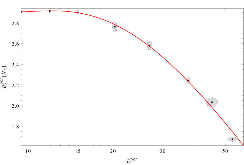
We tried to fit our data for B4pcr[N2](N4)superscriptsubscript𝐵4𝑝𝑐𝑟delimited-[]subscript𝑁2subscript𝑁4B_{4}^{pcr}\mathop{\left[N_{2}\right]}\mathop{\left(N_{4}\right)} assuming 1stsuperscript1st1^{\text{st}} and 2ndordersuperscript2ndorder2^{\text{nd}}\,\text{order} scaling ansaetze (see Figs. 5 and 5). As is typical for a weak 1stordersuperscript1storder1^{\text{st}}\,\text{order} transition, the 2ndordersuperscript2ndorder2^{\text{nd}}\,\text{order} fit seems to work fine, but the obtained values B4cr[N2]=4.2± 5.0superscriptsubscript𝐵4𝑐𝑟delimited-[]subscript𝑁2plus-or-minus4.25.0B_{4}^{cr}\mathop{\left[N_{2}\right]}\,=\,-4.2\,\pm\,5.0 and ν= 1/dHω= 2.01± 0.74𝜈1subscript𝑑𝐻𝜔plus-or-minus2.010.74\nu\,=\,1/d_{H}\omega\,=\,2.01\,\pm\,0.74 do not make much sense. Now, fixing ω=1𝜔1\omega=1 for the 1stordersuperscript1storder1^{\text{st}}\,\text{order} ansatz, it is not possible to obtain B4cr[N2]=1superscriptsubscript𝐵4𝑐𝑟delimited-[]subscript𝑁21B_{4}^{cr}\mathop{\left[N_{2}\right]}=1 from a fit, not even when using only the data points from the largest two simulated systems: in this case we obtain B4cr[N2]0.7superscriptsubscript𝐵4𝑐𝑟delimited-[]subscript𝑁20.7B_{4}^{cr}\mathop{\left[N_{2}\right]}\approx 0.7.

Refer to caption
Figure 4: Binder cumulant B4pcr[N2]superscriptsubscript𝐵4𝑝𝑐𝑟delimited-[]subscript𝑁2B_{4}^{pcr}\mathop{\left[N_{2}\right]} as a function of 1/N41subscript𝑁41/N_{4}. The red lines correspond to fits of the form (8) with ω=1𝜔1\omega=1 (1stordersuperscript1storder1^{\text{st}}\,\text{order} transition) to the data of the largest and second largest pair of systems. The value B4cr[N2]0.7superscriptsubscript𝐵4𝑐𝑟delimited-[]subscript𝑁20.7B_{4}^{cr}\mathop{\left[N_{2}\right]}\approx 0.7 obtained from the largest pair is too small, whereas the fit for the second largest pair yields a too large value: B4cr[N2]1.6superscriptsubscript𝐵4𝑐𝑟delimited-[]subscript𝑁21.6B_{4}^{cr}\mathop{\left[N_{2}\right]}\approx 1.6.
Refer to caption
Figure 5: Binder cumulant B4pcr[N2]superscriptsubscript𝐵4𝑝𝑐𝑟delimited-[]subscript𝑁2B_{4}^{pcr}\mathop{\left[N_{2}\right]} as a function of average linear system size Lpcr(N4)superscript𝐿𝑝𝑐𝑟subscript𝑁4L^{pcr}\mathop{\left(N_{4}\right)}, assuming a 2ndordersuperscript2ndorder2^{\text{nd}}\,\text{order} transition, together with a fit of the form (8) where N4ω=(Lpcr)1/νsuperscriptsubscript𝑁4𝜔superscriptsuperscript𝐿𝑝𝑐𝑟1𝜈N_{4}^{\omega}=\mathop{\left(L^{pcr}\right)}^{1/\nu}. We also included higher order corrections. It can be seen that the fit seems to work fine, but the obtained values B4cr[N2]=4.2± 5.0superscriptsubscript𝐵4𝑐𝑟delimited-[]subscript𝑁2plus-or-minus4.25.0B_{4}^{cr}\mathop{\left[N_{2}\right]}\,=\,-4.2\,\pm\,5.0 and ν= 2.01± 0.74𝜈plus-or-minus2.010.74\nu\,=\,2.01\,\pm\,0.74 do not make much sense.

As the Binder cumulant involves a 4thordersuperscript4thorder4^{\text{th}}\,\text{order} moment, it requires rather large statistics which we probably have not accumulated yet for the largest system. A fit to the data of the next smaller pair of systems, i.e. those consisting of 48k and 32k 4-simplices, leads to B4cr[N2]1.6superscriptsubscript𝐵4𝑐𝑟delimited-[]subscript𝑁21.6B_{4}^{cr}\mathop{\left[N_{2}\right]}\approx 1.6, which shows that our systems are presumably still too small and we will have to include higher order scaling corrections to obtain a meaningful fit.

4 Conclusion

Our study confirms the qualitative findings of [3, 4]: for κ2κ2pcr(N4)subscript𝜅2superscriptsubscript𝜅2𝑝𝑐𝑟subscript𝑁4\kappa_{2}\,\approx\,\kappa_{2}^{pcr}\mathop{\left(N_{4}\right)} we find for N4 32subscript𝑁432N_{4}\,\geq\,32k a clear double peak structure in the N2subscript𝑁2N_{2} distribution, which becomes more pronounced with increasing system size (and there is no sign that the two peaks will eventually merge again in the thermodynamic limit). This is characteristic of a weak 1stordersuperscript1storder1^{\text{st}}\,\text{order} transition. But the standard 1stordersuperscript1storder1^{\text{st}}\,\text{order} ansatz for finite-size scaling of B4pcr[N2]superscriptsubscript𝐵4𝑝𝑐𝑟delimited-[]subscript𝑁2B_{4}^{pcr}\mathop{\left[N_{2}\right]} did not work so far; presumably our systems are still too small and we have to include higher order scaling corrections.

References

  • [1] J. Ambjorn, J. Jurkiewicz, Four-dimensional simplicial quantum gravity, Phys. Lett. B 278, 42-50 (1992)
  • [2] B. Bruegmann, Monte Carlo simulations of 4d simplicial quantum gravity, J. Math. Phys. 36, 6340-6352 (1995), arXiv:hep-lat/9504004
  • [3] P. Bialas, Z. Burda, A. Krzywicki, B. Petersson, Focusing on the Fixed Point of 4D Simplicial Gravity, Nucl. Phys. B 472, 293-308 (1996), arXiv:hep-lat/9601024
  • [4] B. V. de Bakker, Further evidence that the transition of 4D dynamical triangulation is 1st order, Phys. Lett. B 389, 238-242 (1996), arXiv:hep-lat/9603024
  • [5] B. V. de Bakker, Simplicial Quantum Gravity, arXiv:hep-lat/9508006
  • [6] B. Bauer, E. Gull, S. Trebst, M. Troyer, D. A. Huse, Optimized broad-histogram simulations for strong first-order phase transitions: Droplet transitions in the large-Q Potts model, J. Stat. Mech. P01020 (2010), arXiv:0912.1192 [cond-mat.stat-mech]
  • [7] A.M. Ferrenberg, R.H. Swendsen, New Monte Carlo technique for studying phase transitions, Phys. Rev. Lett. 63, p. 1658 (1989)
  • [8] K. Binder, K. Vollmayr, H.-P. Deutsch, J. D. Reger, M. Scheucher, D. P. Landau, Monte Carlo Methods for First Order Phase Transitions: Some Recent Progress, Int. J. Mod. Phys. C 3 (5), 1025-1058 (1992)