Describing orbit space of global unitary actions for mixed qudit states

Abstract

The unitary $\mathrm{U}(d)\--$equivalence relation on the space $\mathfrak{P}_{+}\,$ of mixed states of $d$-dimensional quantum system defines the orbit space $\mathfrak{P}_{+}/\mathrm{U}(d)\,$ and provides its description in terms the ring $\mathbb{R}[\mathfrak{P}_{+}]^{\mathrm{U}(d)}\,$ of $\mathrm{U}(d)$-invariant polynomials. We prove that the semi-algebraic structure of $\mathfrak{P}_{+}/\mathrm{U}(d)\,$ is determined completely by two basic properties of density matrices, their semi-positivity and Hermicity. Particularly, it is shown that the Procesi-Schwarz inequalities in elements of integrity basis for $\mathbb{R}[\mathfrak{P}_{+}]^{\mathrm{U}(d)}\,$ defining the orbit space, are identically satisfied for all elements of $\mathfrak{P}_{+}$.

1 Introduction

The basic symmetry of isolated quantum systems is the unitary invariance. It sets the equivalence relations between the states and defines the physically relevant factor space. For composite systems implementation of this symmetry has very specific features leading to a such non-trivial phenomenon as the entanglement of quantum states.

The space of mixed states, $\mathfrak{P}_{+}\,,$ of $d$-dimensional binary quantum system is locus in quo for two unitary groups action: the group $\mathrm{U}(d)$ and the tensor product group $\mathrm{U}(d_{1})\otimes\mathrm{U}(d_{2})\,,$ where $d_{1},d_{2}$ stand for dimensions of subsystems, $d=d_{1}d_{2}$. Both groups act on a state $\varrho\in\mathfrak{P}_{+}\,$ in adjoint manner

$$(\mathrm{Ad}\,g\,)\varrho=g\,\varrho\,g^{-1}\,.$$ (1)

As a result of this action one can consider two equivalent classes of $\varrho$; the global $\mathrm{U}(d)\--$orbit and the local $\mathrm{U}(d_{1})\otimes\mathrm{U}(d_{2})\--$orbit. The collection of all $\mathrm{U}(d)$-orbits, together with the quotient topology and differentiable structure defines the “global orbit space”, $\mathfrak{P}_{+}/\mathrm{U}(d)\,,$ while the orbit space $\mathfrak{P}_{+}/\mathrm{U}(d_{1})\otimes\mathrm{U}(d_{2})$  represents the “local orbit space” , or the so-called entanglement space $\mathcal{E}_{d_{1}\times d_{2}}$. The latter space is proscenium for manifestations of the intriguing effects occurring in quantum information processing and communications.

Both orbit spaces admit representations in terms of the elements of integrity basis for the corresponding ring of $\mathrm{G}$-invariant polynomials, where $\mathrm{G}$ is either $\mathrm{G}=\mathrm{U}(d)$ or $\mathrm{G}=\mathrm{U}(d_{1})\otimes\mathrm{U}(d_{2})$. This can be done implementing the Procesi and Schwarz method, introduced in 80th of last century for description of the orbit space of a compact Lie group action on a linear space [1, 2]. According to the Procesi and Schwarz the orbit space is identified with the semi-algebraic variety, defined by the syzygy ideal for the integrity basis and the semi-positivity condition of a special, so-called “gradient matrix”, $\mathrm{Grad}(z)\geqslant 0\,,$ that is constructed from the integrity basis elements. In the present note we address the question of application of this generic approach to the construction of $\mathfrak{P}_{+}\,/\mathrm{U}(d)\,$ and $\mathfrak{P}_{+}/\mathrm{U}(d_{1})\otimes\mathrm{U}(d_{2})$. Namely, we study whether the semi-positivity of $\mathrm{Grad}\--$ matrix introduces new conditions on the elements of the integrity basis for the corresponding ring $\mathbb{R}[\mathfrak{P}_{+}]^{\mathrm{G}}$. Below it will be shown that for the global unitary invariance, $\mathrm{G}=\mathrm{U}(d)\,,$ the semi-algebraic structure of the orbit space is determined solely from the physical conditions on density matrices, their semi-positivity and Hermicity. The conditions $\mathrm{Grad}(z)\geqslant 0\,$ do not bring new restrictions on the elements of integrity basis for $\mathbb{R}[\mathfrak{P}_{+}]^{\mathrm{U}(d)}\,.$ Opposite to this case, for the local symmetries the Procesi and Schwarz inequalities impact on the algebraic and geometric properties of the entanglement space.

Our presentation is organized as follows. In section 2 the Procesi and Schwarz method is briefly stated in the form applicable to analysis of adjoint unitary action on the space of states. In section 3 the semi-algebraic structure of $\mathfrak{P}_{+}/\mathrm{U}(d)\,$ is discussed. The final section is devoted to a detailed consideration of two examples, the orbit space of qutrit (d=3) and the global orbit space of four-level quantum system (d=4).

2 The Procesi-Schwarz method

Here we briefly state the above mentioned method for the orbit space construction elaborated by Procesi and Schwartz for the case of compact Lie group action on a linear space [1, 2].

Consider a compact Lie group G acting linearly on the real $d$-dimensional vector space $V$. Let $\mathbb{R}[V]^{\mathrm{G}}$ is the corresponding ring of the $\mathrm{G}$-invariant polynomials on $V$. Assume ${\cal P}=\left(p_{1},p_{2},\dots,p_{q}\right)$ is a set of homogeneous polynomials that form the integrity basis,

$$\mathbb{R}[x_{1},x_{2},\dots,x_{d}]^{\mathrm{G}}=\mathbb{R}[p_{1},p_{2},\dots,p_{q}]\,.$$

Elements of the integrity basis define the polynomial mapping:

$$p:\qquad V\rightarrow\mathbb{R}^{q}\,;\qquad(x_{1},x_{2},\dots,x_{d})\rightarrow(p_{1},p_{2},\dots,p_{q})\,.$$ (2)

Since $p$ is constant on the orbits of $\mathrm{G}$ it induces a homeomorphism of the orbit space $V/G$ and the image $X$ of $p$-mapping; $V/G\simeq X$ [1, 2]. In order to describe $X$ in terms of ${\cal P}$ uniquely, it is necessary to take into account the syzygy ideal of ${\cal P},$ i.e.,

$$I_{\cal P}=\{h\in\mathbb{R}[y_{1},y_{2},\dots,y_{q}]\ :\ h(p_{1},p_{2},\dots,p_{q})=0\,\}\subseteq\mathbb{R}[V]\,.$$

Let $Z\subseteq\mathbb{R}^{q}$ denote the locus of common zeros of all elements of $I_{\cal P}\,,$ then $Z$ is affine variety in $\mathbb{R}^{q}\,$ such that $X\subseteq Z$. Denote by $\mathbb{R}[Z]$ the coordinate ring of $Z$, that is, the ring of polynomial functions on $Z$. Then the following isomorphism takes place [3]

$$\mathbb{R}[Z]\simeq\mathbb{R}[y_{1},y_{2},\dots,y_{q}]/I_{\cal P}\simeq\mathbb{R}[V]^{\mathrm{G}}\,.$$

Therefore, the subset $Z$ essentially is determined by $\mathbb{R}[V]^{\mathrm{G}}$, but to describe $X$ the further steps are required. According to [1, 2] the necessary information on $X$ is encoded in the semi-positivity of $q\times q$ matrix with elements given by the inner products of gradients, $\mathrm{grad}(p_{i}):$

$$||\mathrm{Grad}||_{ij}=\left(\mathrm{grad}\left(p_{i}\right),\mathrm{grad}\left(p_{j}\right)\right)\,.$$

Briefly summarizing all above, the G-orbit space can be identified with the semi-algebraic variety, defined as points, satisfying two conditions:

• $z\in Z$, where $Z$ is the surface defined by the syzygy ideal for the integrity basis of $\mathbb{R}[V]^{\mathrm{G}}$;

• $\mathrm{Grad}(z)\geqslant 0\,.$

Having in mind these basic facts one can pass to the construction of the orbit space $\mathfrak{P}_{+}/\mathrm{U}(d)\,.$ At first we describe the generic semi-algebraic structure and further exemplify it considering two simple, three and four level quantum systems.

3 Semi-algebraic structure of $\mathfrak{P}_{+}/\mathrm{U}(d)\,$

The first step making the Procesi-Schwarz method applicable to the case we are interested in consists in the linearization of the adjoint $\mathrm{U}(d)\--$action (1). For the unitary action one can achieve this as follows. Consider the space $\mathcal{H}_{d\times d}\,$ of $d\times d$ Hermitian matrices and define the mapping

$$\mathcal{H}_{d\times d}\to\mathbb{R}^{d^{2}}\,;\qquad\varrho_{11}=v_{1},\varrho_{12}=v_{2},\dots,\varrho_{1d}=v_{d},\varrho_{21}=v_{d+1}\dots,\varrho_{dd}=v_{d^{2}}\,.$$

Then it can be easily verified that the linear representation on $\mathbb{R}^{d^{2}}$

$$\boldsymbol{v}^{\prime}=L\boldsymbol{v}\,,\qquad L\in\mathrm{U}(d)\otimes\overline{\mathrm{U}(d)}\,,$$

where a line over expression means the complex conjugation, is isomorphic to the initial adjoint $\mathrm{U}(d)$ action (1).

Now the corresponding integrity basis ${\cal P}=\left(p_{1},p_{2},\dots,p_{q}\right)$ for the ring of invariant polynomials is required for the mapping (2). For its construction the following observation is in order. Starting from the center $\mathcal{Z}(\mathfrak{su}(\mathrm{d}))\,$ of the universal enveloping algebra $\mathfrak{U}(\mathfrak{su}(\mathrm{d}))$, according to the well-known Gelfand’s theorem, one can define an isomorphic commutative symmetrized algebra of invariants $S(\mathfrak{su}(\mathrm{d}))\,$, which by turn is isomorphic to the algebra of invariant polynomials over $\mathfrak{su}(\mathrm{d})$ [4]. The later provides the required resource for coordinates that can be used to parameterize the orbit space $\mathfrak{P}_{+}/\mathrm{U}(d)\,.$ For our purpose it is convenient to choose the integrity basis that is formed by the so-called trace invariants. Namely, we use below the polynomial ring $\mathbb{R}[v_{1},v_{2},\dots,v_{d^{2}}]^{\mathrm{U}(d)}=\mathbb{R}[t_{1},t_{2},\dots,t_{d}]\,,$ with n basis elements

$$t_{k}=\mbox{tr}\left(\varrho^{k}\right)\,,\qquad k=1,2.\dots,d\,.$$ (3)

In terms of the integrity basis (3) the $\mbox{Grad}\--$matrix reads

$$\mbox{Grad}(t_{1},t_{2},\dots,t_{d})=\left(\begin{array}[]{ccccc}d&2t_{1}&3t_{2}&\cdots&dt_{d-1}\\ 2t_{1}&2^{2}t_{2}&2\cdot 3t_{3}&\cdots&2\cdot dt_{d}\\ 3t_{2}&2\cdot 3t_{3}&3^{2}t_{4}&\cdots&3\cdot dt_{d+1}\\ \vdots&\vdots&\vdots&\vdots\,\vdots\,\vdots&\\ dt_{d-1}&2\cdot dt_{d}&3\cdot dt_{d+1}&\cdots&d^{2}t_{2d-2}\\ \end{array}\right)\,.$$ (4)

In (4) polynomials $t_{k}$ with $k>d$ are expressed as polynomials in $(t_{1},t_{2},\dots,t_{d})$. From (4) one can easily obtain that

$$\mbox{Grad}(t_{1},t_{2},\dots,t_{d})=\chi\mbox{Disc}\left(t_{1},t_{2},\dots,t_{d}\right)\chi^{T}\,,$$ (5)

where $\chi=\left(1,2,\dots,d\right)\,$ and $\mbox{Disc}\left(t_{1},t_{2},\dots,t_{d}\right)$ denotes the matrix

$$\mbox{Disc}\left(t_{1},t_{2},\dots,t_{d}\right)=\left(\begin{array}[]{ccccc}d&t_{1}&t_{2}&\cdots&t_{d-1}\\ t_{1}&t_{2}&t_{3}&\cdots&t_{d}\\ t_{2}&t_{3}&t_{4}&\cdots&t_{d+1}\\ \vdots&\vdots&\vdots&\vdots\,\vdots\,\vdots&\\ t_{d-1}&t_{d}&t_{d+1}&\cdots&t_{2d-2}\\ \end{array}\right)\,.$$ (6)

In one’s turn the matrix (6) can be written as “square” of the Vandermonde matrix, $\mbox{Disc}\left(t_{1},t_{2},\dots,t_{d}\right)\ =\Delta\Delta^{T}\,,$

$$\Delta(x_{1},\dots,x_{d})=\left(\begin{array}[]{ccccc}1&x_{1}&x_{1}^{2}&\dots&x_{1}^{d-1}\\ 1&x_{2}&x_{2}^{2}&\dots&x_{2}^{d-1}\\ 1&x_{3}&x_{3}^{2}&\dots&x_{3}^{d-1}\\ \vdots&\vdots&\vdots&\vdots\,\vdots\,\vdots&\\ 1&x_{d}&x_{d}^{2}&\dots&x_{d}^{d-1}\\ \end{array}\right)\,,$$ (7)

whose columns are determined by powers of roots $(x_{1},x_{2},\dots x_{d})$ of the characteristic equation:

$$\det||x-\varrho||=x^{d}-S_{1}x^{d-1}+S_{2}x^{d-2}-\dots+(-1)^{d}\,S_{d}=0\,.$$ (8)

The semi-positivity condition of the matrix (6) guaranties reality of the roots of (8). Thus, semi-positivity of the $\mbox{Grad}\--$matrix is equivalent to the reality condition of eigenvalues of the density matrix $\varrho$ written in terms of the $\mathrm{U}(d)$ polynomial scalars. Finally, noting that the density matrices by construction are Hermitian, we convinced that the Procesi-Schwarz inequalities are satisfied identically on $\mathfrak{P}_{+}\,.$

Summarizing, the algebraic structure of the orbit space $\mathfrak{P}_{+}/\mathrm{U}(d)\,$ is completely determined by the inequalities in elements of the integrity basis for polynomial ring $\mathbb{R}[t_{1},t_{2},\dots,t_{d}]$ originating from the Hermicity and semi-positivity requirements on density matrices.

4 Two examples

Algebraic structure of the orbit space of quantum systems is highly intricate. The examples of d=3 (qutrit) and d=4, considered below, demonstrate the degree of its complexity even for the low dimensional systems.

4.1 Orbit space of qutrit

Qutrit is 3-dimensional quantum system and the integrity basis for $\mathrm{U}(3)$-invariant polynomial consist from first, second and third order trace polynomials; $t_{1},t_{2},t_{3}\,.$ For a visibility below we consider the case of normalized density matrices, supposing $t_{1}=1.$

The condition of the eigenvalues reality is

$$0\leq\frac{1}{6}\left(3t_{2}^{3}-21t_{2}^{2}+36t_{3}t_{2}+9t_{2}-18t_{3}^{2}-8t_{3}-1\right)\,,$$ (9)

while the semi-positivity of density matrices formulated as non-negativity of coefficients of characteristic equation (8) reads

$$0\leq\tfrac{1}{2}(1-t_{2})\leq\tfrac{1}{3}\,,$$

$$0\leq\tfrac{1}{2}(1-3t_{2}+2t_{3})\leq\tfrac{1}{9}\,.$$

Resolving the inequalities

Red domain: $$\qquad\tfrac{1}{3}\leq t_{2}\leq 1$$

Yellow domain: $$\qquad 3t_{2}-1\leq 2 t_{3}\leq 3t_{2}-\tfrac{7}{9}$$

Green domain: $$\qquad-4+18t_{2}-\sqrt{2}(3t_{2}-1)^{3/2}\leq 18 t_{3}\leq-4+18t_{2}+\sqrt{2}(3t_{2}-1)^{3/2}$$

we get the intersection domain shown on Figure 1.

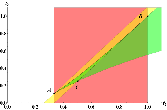
Figure 1: Triangle domain A-B-C as the orbit space of qutrit.

The triangle domain A-B-C, bounded by the lines:

A-B $$t_{3}=\tfrac{1}{18}(-4+18t_{2}+\sqrt{2}(3t_{2}-1)^{3/2})$$

A-C $$t_{3}=\tfrac{1}{18}(-4+18t_{2}-\sqrt{2}(3t_{2}-1)^{3/2})$$

B-C $$t_{3}=\tfrac{3}{2}t_{2}-\tfrac{1}{2}$$

with vertexes : $A(\tfrac{1}{3},\tfrac{1}{9})\,,$ $B(1,1)\,$ and $C(\tfrac{1}{2},\tfrac{1}{4})\,,$ represents the orbit space of qutrit in parametrization of trace polynomial coordinates.

Now it is in order to discuss correspondence between the above algebraic results and known classification of orbits with respect to their stability group. Having in mind this issue consider the Bloch parametrization for qutrit

$$\rho=\frac{1}{3}\left(\mathbb{I}_{3}+\sqrt{3}\,\boldsymbol{\xi}\cdot\boldsymbol{\lambda}\right),$$ (10)

where $\boldsymbol{\xi}=(\xi_{1},\xi_{2},\cdots,\xi_{8})\in\mathbb{R}^{8}$ denote the Bloch vector and $\boldsymbol{\lambda}$ is the vector, whose components are elements $(\lambda_{1},\lambda_{2},\cdots,\lambda_{8})$ of $\mathfrak{su}(3)$ algebra basis, say the Gell-Mann matrices,

$$\begin{array}[]{c}\begin{array}[]{ccc}\lambda_{1}=\left(\begin{array}[]{ccc}0&1&0\\ 1&0&0\\ 0&0&0\end{array}\right)&\lambda_{2}=\left(\begin{array}[]{ccc}0&-i&0\\ i&0&0\\ 0&0&0\end{array}\right)&\lambda_{3}=\left(\begin{array}[]{ccc}1&0&0\\ 0&-1&0\\ 0&0&0\end{array}\right)\\ &&\\ \lambda_{4}=\left(\begin{array}[]{ccc}0&0&1\\ 0&0&0\\ 1&0&0\end{array}\right)&\lambda_{5}=\left(\begin{array}[]{ccc}0&0&-i\\ 0&0&0\\ i&0&0\end{array}\right)&\lambda_{6}=\left(\begin{array}[]{ccc}0&0&0\\ 0&0&1\\ 0&1&0\end{array}\right)\end{array}\\ \\ \begin{array}[]{cc}\lambda_{7}=\left(\begin{array}[]{ccc}0&0&0\\ 0&0&-i\\ 0&i&0\end{array}\right)&\lambda_{8}=\displaystyle{\frac{1}{\sqrt{3}}}\left(\begin{array}[]{ccc}1&0&0\\ 0&1&0\\ 0&0&-2\end{array}\right)\end{array}\end{array}\,,$$ (11)

obeying

$$[\lambda_{i},\lambda_{j}]=2\imath f_{ijk}\lambda_{k}\,,\qquad\mbox{tr}\left(\lambda_{i}\lambda_{j}\right)=2\delta_{ij}\,,$$ (12)

with non-vanishing structure constants

$$f_{123}=2f_{147}=2f_{246}=2f_{257}=2f_{345}=-2f_{156}=-2f_{367}=\frac{2}{\sqrt{3}}f_{458}=\frac{2}{\sqrt{3}}f_{678}=1\,.$$ (13)

Yo analyse the adjoint orbit $\cal{O}_{\varrho}\,$ that passes through the point $\varrho$, we define the set of tangent vectors:

$$l_{i}=\lim_{\theta_{1},\theta_{2},\dots\theta_{8}\to 0}\,\frac{\partial}{\partial\theta_{i}}\left[U\left(\theta_{1},\theta_{2},\dots\theta_{8}\right)\,\varrho\,U\left(\theta_{1},\theta_{2},\dots\theta_{8}\right)\right]=\imath[\lambda_{i},\varrho]\,.$$ (14)

By definition, the dimension of orbit $\mbox{dim}(\mathcal{O}_{\varrho})$ is given by the dimension of the tangent space to the orbit $T_{\mathcal{O}_{\varrho}}$ and therefore equals to the the number of linearly independent vectors among eight tangent vectors $l_{1},l_{2},\dots,l_{8}\,.$ This number depends on the point $\varrho$ and according to the well-known theorem from linear algebra is given by the rank of the so-called Gram matrix

$$A_{ij}=\frac{1}{2}\,\|\mbox{tr}(l_{i}l_{j})\|\,.$$ (15)

In the Bloch parameterization (10) we easily find that

$$A_{ij}=\frac{4}{3}\,f_{ims}f_{jns}\xi_{m}\xi_{n}\,.$$ (16)

To estimate the rank of matrix (15) it is convenient to pass to the diagonal representative of the matrix $\varrho$:

$$\varrho=W\left(\begin{array}[]{ccc}x_{1}&0&0\\ 0&x_{2}&0\\ 0&0&x_{3}\\ \end{array}\right)W^{+}\,,$$ (17)

where $W\in\mathrm{SU(3)}/S_{3}$ and the descending order for $\varrho$ matrix eigenvalues

$$1\geq x_{1}\geq x_{2}\geq x_{3}\geq 0\,,$$

is chosen. The later constraints allow to avoid a double counting due to the $S_{3}\subset U(3)$ symmetry of permutation of the density matrix eigenvalues. Using the principal axis transformation (17) and taking into account the adjoint properties of Gell-Mann matrices $W^{+}\lambda_{i}W=O_{ij}\lambda_{j}\,,$ with $O\in SO(8)\,,$ the matrix $A_{ij}$ can be written as

$$A_{ij}=O_{ik}A^{\mathrm{diag}}_{kl}O^{T}_{lj}\,.$$ (18)

Matrix $A^{\mathrm{diag}}_{kl}$ in (18) is the matrix (15) constructed from vectors $l^{\mathrm{diag}}_{i}=i[\lambda_{i},\varrho_{\mathrm{diag}}]$ tangent to the orbit of the diagonal matrix $\varrho_{\mathrm{diag}}:=\mbox{diag}(x_{1},x_{2},x_{3})\,.$

Since we are interesting in determination of $\mbox{rank}|A|$, the relation (18) allows to reduce this question to the evaluation of the rank of the diagonal representative $\varrho_{\mathrm{diag}}\,.$ For diagonal matrices the Bloch vector is $\boldsymbol{\xi}^{\mathrm{diag}}=(0,0,0,\xi_{3},0,0,0,\xi_{8})$. Taking into account the values for structure constants from (13), the expression for $|A^{\mathrm{diag}}|$ reads

$$A^{\mathrm{diag}}=\frac{1}{3}\,\mbox{diag}\left(4\xi_{3}^{2},4\xi_{3}^{2},0,(\xi_{3}+\sqrt{3}\xi_{8})^{2},(\xi_{3}+\sqrt{3}\xi_{8})^{2},(\xi_{3}-\sqrt{3}\xi_{8})^{2},(\xi_{3}-\sqrt{3}\xi_{8})^{2},0\right)\,.$$ (19)

From (19) we conclude that there are orbits of three different dimensions:

• the orbits of maximal dimension, $\mbox{dim}(\mathcal{O}_{\varrho})=6\,,$

• the orbits of dimension, $\mbox{dim}(\mathcal{O}_{\varrho})=4\,,$

• zero dimensional orbit, one point $\boldsymbol{\xi}=0\,.$

The above algebraic description of the orbits $\mathcal{O}_{\varrho}$ corresponds to their classification based on the analysis of the group of transformations $\mathrm{G}_{\varrho}$– the isotropy group (or stability group), which stabilize point $\varrho\in\mathcal{O}_{\varrho}$. The orbits of different dimensions have a different stability groups; for the points lying on the orbit of maximal dimension the stability group is the Cartan subgroup $\mathrm{U(1)}\otimes\mathrm{U(1)}\otimes\mathrm{U(1)}$, while the stability group of points with diagonal representative $\lambda_{8}$ is $\mathrm{U(2)}\otimes\mathrm{U(1)}$. The dimensions of listed orbits agrees with the general formula

$$\mathrm{dim}\,\mathcal{O}_{\varrho}=\mathrm{dimG}-\mathrm{dim{G}_{\varrho}}\,.$$ (20)

Since the isotropy group of any two points on the orbit are the same up to conjugation, the orbits can be partitioned into sets with equivalent isotropy groups . This set is known as “strata”.

Concluding we refer to the relations between the triangle A-B-C, depicted on the Figure 1, and the corresponding strata. The domain inside the triangle ABC corresponds to the principal strata with the stability group $U(1)\times U(1)\times U(1)$. The discriminant is positive $|\mbox{Disc}|>0$ and the density matrix has three different real eigenvalues, the representative matrix reads $\frac{1}{3}(\mathbb{I}_{3}+\sqrt{3}\left(\xi_{3}\lambda_{3}+\xi_{8}\lambda_{8}\right))$, with $\xi_{3}$ and $\xi_{8}$ subject to the following constraints

$$0<1-\xi_{3}^{2}-\xi_{8}^{2}<1\,,\qquad 0<(2\xi_{8}-1)(1-\sqrt{3}\xi_{3}+\xi_{8})(1+\sqrt{3}\xi_{3}+\xi_{8})<1\,.$$

The $S_{3}$ coefficient vanishes at line B-C. The boundary line B-C, excluding vertices B and C also belongs to the principal stratum, while points B and C belong to the stratum of lower dimension. On the sides A-B and A-C the discriminant is zero $|\mbox{Disc}|=0$, hence, the density matrix has three real eigenvalues and two of them are equal. At point B two eigenvalues of $\varrho$ are zero. The lines (A-B)/{A} and (A-C)/{A} represent the degenerate 4-dimensional orbits whose stability group is $U(2)\otimes U(1)$. Finally, the point A is the zero dimensional stratum corresponding to the maximally mixed state $\varrho=\frac{1}{3}\mathbb{I}_{3}$. The details of the orbit types are collected in the Table below.

$$\begin{array}[]{c|c|c|c|c}\dim\mathcal{O}&\mbox{Strata}&\mbox{\parbox{85.35826pt}{Stability group}}&\mbox{\parbox{113.81102pt}{Representative matrix}}&\mbox{\parbox{99.58464pt}{Constraints}}\\[19.91692pt] \hline\cr\hline\cr\rule{-4.0pt}{30.0pt}6&\begin{array}[]{c}\mbox{Interior~{}of }\\ \mbox{triangle}\\ \mbox{ABC}\end{array}&U(1)\otimes U(1)\otimes U(1)&\frac{1}{3}(\mathbb{I}_{3}+\sqrt{3}\left(\xi_{3}\lambda_{3}+\xi_{8}\lambda_{8}\right))&{\mbox{Disc}>0,S_{2}>0,S_{3}>0}\\[19.91692pt] \cline{2-5}\cr\rule{-4.0pt}{30.0pt}&\mbox{\parbox{71.13188pt}{Boundary: (B-C)/\{B,C\}}}&U(1)\otimes U(1)\otimes U(1)&\frac{1}{3}(\mathbb{I}_{3}+\sqrt{3}\left(\xi_{3}\lambda_{3}+\frac{1}{2}\lambda_{8}\right))&{\mbox{Disc}>0,S_{2}>0,S_{3}=0}\\[19.91692pt] \hline\cr\rule{-4.0pt}{35.0pt}4&\begin{array}[]{c}\mbox{Boundary:}\\ \mbox{(A-B)/\{A\}}\\ \mbox{(A-C)/\{A\}}\end{array}&U(2)\otimes U(1)&\begin{array}[]{c}\frac{1}{3}(\mathbb{I}_{3}+\sqrt{3}\,\xi_{8}\lambda_{8})\end{array}&{\mbox{Disc}=0,S_{2}\geq 0,S_{3}\geq 0}\\[25.60747pt] \hline\cr\rule{-4.0pt}{30.0pt}0&\mbox{\parbox{56.9055pt}{Point: \{A\}}}&U(3)&\frac{1}{3}\mathbb{I}_{3}&\mbox{Disc}=S_{2}=S_{3}=0\\[25.60747pt] \hline\cr\end{array}$$

Table. The stratum decomposition for the orbit space of qutrit.

4.2 Orbit space of a four-level quantum system

The density matrix $\varrho$ of a $4$-level quantum system in the Bloch form reads

$$\rho=\frac{1}{4}\left(\mathbb{I}_{4}+\sqrt{6}\,\vec{\xi}\cdot\vec{\lambda}\right)\,,$$ (21)

where the traceless part of $\varrho$ is given by scalar product of 15-dimensional Bloch vector $\vec{\xi}=\{\xi_{1},\ldots,\xi_{15}\}\in\mathbb{R}^{15}$ with $\lambda$-vector whose components are elements of the Hermitian basis of the Lie algebra $\mathfrak{su}(4)$

$$\lambda_{i}\lambda_{j}=\frac{1}{2}\,\delta_{ij}\mathbb{I}_{4}+(d_{ijk}+i\,f_{ijk})\lambda_{k},\qquad i,j,k=1,\ldots,15.$$

The corresponding integrity basis for the polynomial ring $\mathbb{R}[\mathfrak{P}_{+}]^{\mathrm{U}(4)}\,$ consists of three $\mathrm{U}(4)$-invariant polynomials, the Casimir scalars $\mathfrak{C}_{2},\mathfrak{C}_{3},\mathfrak{C}_{4}$

$$\mathfrak{C}_{2}=\vec{\xi}\cdot\vec{\xi}\,\qquad\mathfrak{C}_{3}=\sqrt{\frac{3}{2}}\,d_{ijk}\xi_{i}\xi_{j}\xi_{k}\,,\qquad\mathfrak{C}_{4}=\frac{3}{2}\,d_{ijk}d_{lmk}\xi_{i}\xi_{j}\xi_{l}\xi_{m}\,,$$ (22)

The semi-positivity of (21) formulated as non-negativity of coefficients $S_{2},S_{3}$ and $S_{4}$ of the characteristic polynomial (8)

$$S_{2}=\tfrac{3}{8}(1-\mathfrak{C}_{2})\geq 0$$ (23)

$$S_{3}=\tfrac{1}{16}(1-3\mathfrak{C}_{2}+2\mathfrak{C}_{3})\geq 0,$$ (24)

$$S_{4}=\det\rho=\tfrac{1}{256}((1-3\mathfrak{C}_{2})^{2}+8\mathfrak{C}_{3}-12\mathfrak{C}_{4})\geq 0$$ (25)

Now we are in position to compute the Grad-matrix in terms of the $\mathrm{SU(4)}$ Casimir scalars:

$$\mbox{Grad}=\begin{pmatrix}4\mathfrak{C}_{2}&6\mathfrak{C}_{3}&8\mathfrak{C}_{4}\\ 6\mathfrak{C}_{3}&9\mathfrak{C}_{4}&12\mathfrak{C}_{2}\mathfrak{C}_{3}\\ 8\mathfrak{C}_{4}&12\mathfrak{C}_{2}\mathfrak{C}_{3}&4(\mathfrak{C}_{3}^{2}+3\mathfrak{C}_{2}\mathfrak{C}_{4})\\ \end{pmatrix}\,.$$ (26)

Passing to the equivalent matrix $Q\,\mbox{Grad}\,Q^{T}\,,$ with $Q=\mbox{diag}(2,3,2)\,,$ we arrive at the following form for the Procesi-Schwarz inequalities

$$\mathfrak{C}_{2}+\mathfrak{C}_{3}^{2}+3\mathfrak{C}_{2}\mathfrak{C}_{4}+\mathfrak{C}_{4}\geq 0\,,$$ (27)

$$\mathfrak{C}_{3}^{2}\left(-4\mathfrak{C}_{2}^{2}+\mathfrak{C}_{2}+\mathfrak{C}_{4}-1\right)+\mathfrak{C}_{4}\left(3\mathfrak{C}_{2}^{2}+3\mathfrak{C}_{2}\mathfrak{C}_{4}+\mathfrak{C}_{2}-4\mathfrak{C}_{4}\right)\geq 0\,,$$ (28)

$$-4\mathfrak{C}_{2}^{3}\mathfrak{C}_{3}^{2}+3\mathfrak{C}_{2}^{2}\mathfrak{C}_{4}^{2}+6\mathfrak{C}_{2}\mathfrak{C}_{3}^{2}\mathfrak{C}_{4}-\mathfrak{C}_{3}^{4}-4\mathfrak{C}_{4}^{3}\geq 0\,.$$ (29)

The domains describing the semi-positivity of $\rho\,,$ (23)-(25), and its residually part after imposing condition of the semi-positivity of Grad-matrix (27)-(29) are depicted on the Figure 2.

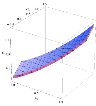
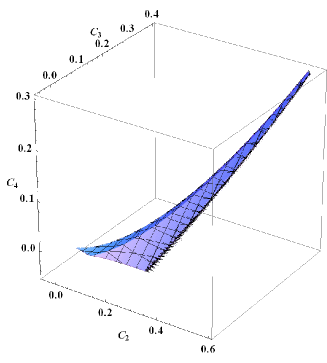
Figure 2: On the left side: $\rho\geq 0$; On the right side: $\rho\geq 0\cap\mbox{Grad}\geq 0$;

$\bullet\,$Acknowledgements $\bullet\,$ The work is supported in part by the Ministry of Education and Science of the Russian Federation (grant 3802.2012.2) and the Russian Foundation for Basic Research (grant 13-01-0068). A. Kh. acknowledges the University of Georgia for support under the grant 07-01-2013.

References

• [1] C. Procesi and G. Schwarz, The geometry of orbit spaces and gauge symmetry breaking in supersymmetric gauge theories, Phys. Lett.  B 161, 117-121 (1985).
• [2] C. Procesi and G. Schwarz, Inequalities defining orbit spaces, Invent.math. 81 539-554 (1985).
• [3] D. Cox, J, Little and D. O’Shea, Ideals, Varieties, and Algorithms, Third Edition, Springer, (2007).
• [4] D. P.Zelobenko, Compact Lie groups and their representation, Translation of Mathematical Monographs, vol. 40, AMS (1978).
• [5] L. Michel and L.A. Radicati, The geometry of the octet, Ann. Inst. Henri Poincare, Section A, 18, 185-214 (1973).
• [6] M.Adelman, J.V.Corbett and C.A.Hurst, The geometry of state space, Foundation of Physics, 23, 211-223 (1993).
• [7] M. Kus and K. Zyczkowski, Geometry of entangled states, Phys. Rev. A 63, 032307, (2008).
• [8] L.J. Boya and K. Dixit, Geometry of density matrix states, Phys. Rev. A 78, 042108 (2008).
• [9] V. Gerdt, A. Khvedelidze and Yu. Palii, On the ring of local polynomial invariants for a pair of entangled qubits, Zapiski POMI  373, 104-123 (2009).