Revealing Relationships among Relevant Climate Variables with Information Theory

Abstract

A primary objective of the NASA Earth-Sun Exploration Technology Office is to understand the observed Earth climate variability, thus enabling the determination and prediction of the climate’s response to both natural and human-induced forcing. We are currently developing a suite of computational tools that will allow researchers to calculate, from data, a variety of information-theoretic quantities such as mutual information, which can be used to identify relationships among climate variables, and transfer entropy, which indicates the possibility of causal interactions. Our tools estimate these quantities along with their associated error bars, the latter of which is critical for describing the degree of uncertainty in the estimates. This work is based upon optimal binning techniques that we have developed for piecewise-constant, histogram-style models of the underlying density functions. Two useful side benefits have already been discovered. The first allows a researcher to determine whether there exist sufficient data to estimate the underlying probability density. The second permits one to determine an acceptable degree of round-off when compressing data for efficient transfer and storage. We also demonstrate how mutual information and transfer entropy can be applied so as to allow researchers not only to identify relations among climate variables, but also to characterize and quantify their possible causal interactions.

1 Introduction

A primary objective of the NASA Earth-Sun Exploration Technology Office is to understand the observed Earth climate variability, and determine and predict the climate’s response to both natural and human-induced forcing. Central to this problem is the concept of feedback and forcing. The basic idea is that changes in one climate subsystem will cause or force responses in other subsystems. These responses in turn feed back to force other subsystems, and so on. While it is commonly assumed that these interactions can be described by linear systems techniques, one must appeal to large-scale averages, asymptotic distributions and central limit theorems to defend such models. In doing so, our ability to describe processes with reasonably high spatiotemporal resolution is lost in the averaging step. There are distinct advantages to developing feedback and forcing models that allow for nonlinearity. This is especially highlighted by the results of Lorenz’s work in modelling convection cells [1], which is used today as a textbook example of a nonlinear system, and historically was instrumental in the development of modern nonlinear dynamics.

In the early stages of a field of science, much effort goes into identifying the relevant variables. This is typically a small set of variables that are used as parameters in idealized scientific models of the physical phenomenon under study. In Galileo’s time, he found that motion was best described by the relevant variables: displacement, velocity, and acceleration. Sometimes these scientific models are gross oversimplifications that merely capture the basic essence of a physical process, and sometimes they are highly detailed and allow one to make specific predictions about the system. In Earth Science, the fact that the majority of our efforts are spent on amassing large amounts of data indicates that we have not yet identified the relevant variables for many of the problems that we study. One of the aims of this work is to develop methods that will enable us to better identify relevant variables.

A second aim of this work is to develop techniques that will allow us to identify relationships among these relevant variables. As mentioned above, it is naive to expect that these variables will interact linearly. Thus techniques that are sensitive to both linear and nonlinear relationships will better enable us to identify interactions among these variables. Information theory allows one to compute the amount of information that knowledge of one variable provides about another [2, 3]. Such computations are applicable to both linear and nonlinear relationships between the variables. Furthermore, they rely on higher-order statistics; whereas approaches such as correlation analysis, Empirical Orthogonal Functions (EOF), Principal Component Analysis (PCA), and Granger causality [4] are based on second-order statistics, which amount to approximating everything with Gaussian distributions. An additional benefit is the fact that higher order generalizations of basic information-theoretic quantities are deeply connected to the concept of relevance [5, 6], and thus this approach is the natural methodology for identifying relevant variables and their interactions with one another.

Information-theoretic computations ultimately rely on quantities such as entropy. While researchers have been estimating entropy from data for years, relatively few attempts have been made to estimate the uncertainties associated with the entropy estimates. We consider this to be of paramount importance, since the degree to which we understand the Earth’s climate system can only be characterized by quantifying our uncertainties. The remainder of this paper will describe our ongoing efforts to estimate information-theoretic quantities from data as well as the associated uncertainties, and to demonstrate how these approaches will be used to identify relationships among relevant climate variables.

2 Density Models

Our knowledge about a variable depends on what we know about the values that it can take. For instance, knowing that the average daytime summer beach water temperature in Hawaii is $80^{\circ}$F provides some information. However, more information would be provided by the variance of this quantity. A complete quantification of our knowledge of this variable would be given by the probability density function. From that, one can compute the probability that the water temperature will fall within a given range. To apply these information-theoretic techniques, we first must estimate the probability density function from a data set.

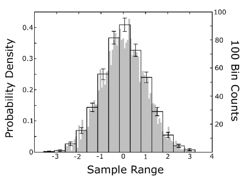
Figure 1: The optimal piecewise-constant probability density model generated from 1000 data samples drawn from a Gaussian density. The error bars indicate the uncertainty in the bin heights. It is superimposed over a 100-bin histogram that shows the irrelevant sampling variations of the data.

2.1 Piecewise-Constant Density Models

We model the density function with a piecewise-constant model. Such a model divides the range of values of the variable into a set of $M$ discrete bins and assigns a probability to each bin. We denote the probability that a data point is found to be in the $k^{th}$ bin by $\pi_{k}$. The result is closely related to a histogram, except that the “height” of the bin $h_{k}$, is the constant probability density (bin probability divided by the bin width) over the region of the bin. Integrating this constant probability density $h_{k}$ over the width of the bin $v_{k}$ leads to a total probability $\pi_{k}=h_{k}v_{k}$ for the bin. This leads to the following piecewise-constant model $h(x)$ of the unknown probability density function for the variable $x$

$$h(x)=\sum_{k=1}^{M}{h_{k}~{}\Pi(x_{k-1},x,x_{k})},$$ (1)

where $h_{k}$ is the probability density of the $k^{th}$ bin with edges defined by $x_{k-1}$ and $x_{k}$, and $\Pi(x_{k-1},x,x_{k})$ is the boxcar function where

$$\Pi(x_{a},x,x_{b})=\left\{\begin{array}[]{rl}0&\mbox{if}~{}~{}x<x_{a}\\ 1&\mbox{if}~{}~{}x_{a}\leq x<x_{b}\\ 0&\mbox{if}~{}~{}x_{b}\leq x\end{array}\right.$$ (2)

For the case of equal bin widths, this density model can be re-written in terms of the bin probabilities $\pi_{k}$ as

$$h(x)=\frac{M}{V}\sum_{k=1}^{M}{\pi_{k}~{}\Pi(x_{k-1},x,x_{k})}.$$ (3)

where $V$ is the width of the entire region covered by the density model. This formalism is readily expanded into multiple dimensions by extending $k$ to the status of a multi-dimensional index, and using $v_{k}$ to represent the multi-dimensional volume, with $V$ representing the multi-dimensional volume covered by the density model.

To accurately describe the density function, we use the data to compute the optimal number of bins. This is performed by applying Bayesian probability theory [7, 8] and writing the posterior probability of the model parameters [9], which are the number of bins $M$ and the bin probabilities $\underline{\pi}=\{\pi_{1},\pi_{2},\ldots,\pi_{M-1}\}$, as a function of the $N$ data points $\underline{d}=\{d_{1},d_{2},\ldots,d_{N}\}$

$$p(\underline{\pi},M|\underline{d},I) \propto\biggl{(}\frac{M}{V}\biggr{)}^{N}\frac{\Gamma\bigl{(}\frac{M}{2}\bigr{)}}{\Gamma\bigl{(}\frac{1}{2}\bigr{)}^{M}}~{}~{}~{}\times$$ (4)

$$\pi_{1}^{n_{1}-\frac{1}{2}}\pi_{2}^{n_{2}-\frac{1}{2}}\ldots\pi_{M-1}^{n_{M-1}-\frac{1}{2}}\biggl{(}1-\sum_{i=1}^{M-1}{\pi_{i}}\biggr{)}^{n_{M}-\frac{1}{2}},$$

where $n_{k}$ is the number of data points in the $k^{th}$ bin. Note that the symbol $I$ is used to represent any prior information that we may have or any assumptions that we have made, such as assuming that the bins are of equal width.

Integrating over all possible bin heights gives the marginal posterior probability of the number of bins given the data [9]

$$p(M|\underline{d},I)\propto\biggl{(}\frac{M}{V}\biggr{)}^{N}\frac{\Gamma\bigl{(}\frac{M}{2}\bigr{)}}{\Gamma\bigl{(}\frac{1}{2}\bigr{)}^{M}}~{}\frac{\prod_{k=1}^{M}{\Gamma(n_{k}+\frac{1}{2})}}{\Gamma(N+\frac{M}{2})},$$ (5)

where the $\Gamma(\cdot)$ is the Gamma function [10, p. 255]. The idea is to evaluate this posterior probability for all the values of the number of bins within a reasonable range and select the result with the greatest probability. In practice, it is often much easier computationally to search for the optimal number of bins $M$ by finding the value of $M$ that maximizes the logarithm of the probability, (5) above.

Using the joint posterior probability (4) one can compute the mean bin probabilities and the standard deviations from the data [9]. The mean bin probability is

$$\mu_{k}=\langle h_{k}\rangle=\frac{\langle\pi_{k}\rangle}{v_{k}}=\biggl{(}\frac{M}{V}\biggr{)}\biggl{(}\frac{n_{k}+\frac{1}{2}}{N+\frac{M}{2}}\biggr{)},$$ (6)

and the associated variance of the height of the $k^{th}$ bin is

$$\sigma_{k}^{2}=\biggl{(}\frac{M}{V}\biggr{)}^{2}\biggl{(}\frac{(n_{k}+\frac{1}{2})(N-n_{k}+\frac{M-1}{2})}{(N+\frac{M}{2}+1)(N+\frac{M}{2})^{2}}\biggr{)},$$ (7)

where the standard deviation is the square root of the variance. Note that bins with no counts still have a non-zero probability. No lack of evidence can ever prove conclusively that an event occurring in a given bin is impossible—just less probable.

In this way we are able to estimate probability densities from data, and quantify the uncertainty in our knowledge. An example of a probability density model is shown in Figure 1. This optimal binning technique ensures that our density model includes all the relevant information provided by the data while ignoring irrelevant details due to sampling variations. The result is the most honest summary of our knowledge about the density function from the given data. Honest representations are important since they can reveal two potentially disastrous situations: insufficient data and excessive round-off error.

2.2 Insufficient Data

Without examining the uncertainties, one can never be sure that one has a sufficient amount of data to make an inference. How many data points does one need to estimate a density function? Do we need $100$ data points? $10000$? a million?

By examining the log posterior probability for the optimal number of bins given the data, one can easily detect whether one possesses sufficient data. In this example (Figure 2), we see two density models constructed from data sampled from a Gaussian distribution. In the first case, we have collected $30$ data points, and in the second case, $1000$. In the case of $30$ data points, the behavior of the log posterior probability, which is the logarithm of (5), is very noisy with spurious maxima. We can not be sure how many bins to use, and are thus very uncertain as to the shape of the density function from which these data were sampled. In the case with $1000$ data points, the behavior of the log posterior is clear. It rises sharply as the number of proposed bins increases and reaches a peak and then gently falls off. The result is an estimate of the number of bins that provides a piecewise-constant density model that, given the data, optimally describes the true “unknown” Gaussian distribution.

In our numerical experiments, we have found that for Gaussian distributed data, one needs approximately $75$ to $100$ data points to get a reasonable solution, and $150$ to $200$ data points to be very certain. Note that this is a different situation than assuming that we know that the underlying distribution is Gaussian and then trying to estimate the mean and variance. That is a very different problem where the prior knowledge that it is Gaussian (which would be represented by that $I$ again) makes is feasible to make the inference using significantly fewer data points.

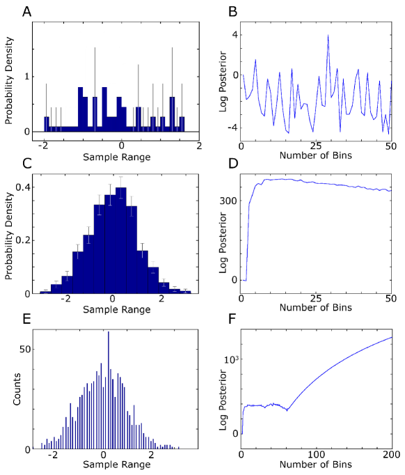
Figure 2: A) With a small number of data points (in this case $30$ data points sampled from a Gaussian), it is not possible to determine the probability density with any accuracy. B) The log posterior in this case jumps around with many spurious local maxima. This indicates that the inference is unreliable and more data are needed. C) With a sufficient amount of data (in this case $1000$ data points), the probability density is easily estimated. D) The log posterior rises rapidly as the number of bins $M$ increases reaching a peak (in this case at $M=14$) and then falling off gently. E) In this example, we take the previous 1000 data points and rounded them off to the nearest $1/10$th. As a result of this severe truncation, the optimal solution looks like a picket fence. The discrete nature of the truncated data is now a more prominent feature than the original probability density function. F) The log posterior detects this once the data have been separated into the discrete bins and can be separated no further.

2.3 Excessive Round-Off

The other problem that can occur is loss of information due to data compression or round-off. Many times to save memory space, data values are truncated to a small number of decimal places. When it is not clear how much information the data contains, it is not clear to what degree the data can be truncated before destroying valuable information. Our optimal binning technique is useful here as well.

In the event that the data has been severely truncated, the optimal binning algorithm will see the discrete structure in the data due as being more meaningful than the overall shape of the underlying density function (Figure 2E). The result is that the optimal number of bins leads to what is called “picket fencing”, where the density model looks like a picket fence. There is no graceful way to recover from this—relevant data has been lost, and cannot be recovered.

3 Entropy and Information

We can characterize the behavior of a system $X$ by looking at the set of states the system visits as it evolves in time. If a state is visited rarely, we would be surprised to find the system there. We can express the expectation (or lack of expectation) to find the system in state $x$ in terms of the probability that it can be found in that state, $p(x)$, by

$$s(x)=\log\frac{1}{p(x)}.$$ (8)

This quantity is often called the surprise, since it is large for improbable events and small for probable ones. Averaging this quantity over all of the possible states of the system gives a measure of our expectation of the state of the system

$$H(X)=\sum_{x\in X}{p(x)\log\frac{1}{p(x)}}.$$ (9)

This quantity is called the Shannon Entropy, or entropy for short [2]. It can be thought of as a measure of the amount of information we possess about the system. It is usually expressed by rewriting the fraction above using the properties of the logarithm

$$H(X)=-\sum_{x\in X}{p(x)\log{p(x)}}.$$ (10)

Note that changing the base of the logarithm merely changes the units in which entropy is measured. When the logarithm base is 2, entropy is measured in bits, and when it is base $e$, it is measured in nats.

If the system states can be described with multiple parameters, we can use them jointly to describe the state of the system. The entropy can still be computed by averaging over all possible states. For two subsystems $X$ and $Y$ the joint entropy is

$$H(X,Y)=-\sum_{x\in X}{\sum_{y\in Y}{p(x,y)\log{p(x,y)}}}.$$ (11)

The differences of entropies are useful quantities. Consider the difference between the joint entropy $H(X,Y)$ and the individual entropies $H(X)$ and $H(Y)$

$$MI(X,Y)=H(X)+H(Y)-H(X,Y).$$ (12)

This quantity describes the difference in the amount of information one possesses when one considers the system jointly instead of considering the system as two individual subsystems. It is called the Mutual Information (MI) since it describes the amount of information that is shared between the two subsystems. If you know something about subsystem $X$, the mutual information describes how much information you also possess about $Y$, and vice versa. Thus MI quantifies the relevance of knowledge about one subsystem to knowledge about another subsystem. For this reason, it is useful for identifying and selecting a set of relevant variables that can aid in the prediction of another climate variable. One should note that if two climate variables X and Y are independent, then $H(X,Y)=H(X)+H(Y)$, then the mutual information (12) is zero—as one would expect. The mutual information is a measure of true statistical independence, whereas concepts like decorrelation only describe independence up to second-order. Two variables can be uncorrelated, yet still dependent.

While the mutual information is an important quantity in identifying relationships between system variables, it provides no information regarding the causality of their interactions. The easiest way to see this is to note that the mutual information is symmetric with respect to interchange of X and Y, whereas causal interactions are not symmetric. To identify causal interactions, a asymmetric quantity must be utilized. Recently, Schreiber [11] introduced a novel information-theoretic quantity called the Transfer Entropy (TE). Consider two subsystems $X$ and $Y$, with data in the form of two time series of measurements

$$X = \{x_{1},x_{2},\ldots,x_{t},x_{t+1},\ldots,x_{n}\}$$

$$Y = \{y_{1},y_{2},\ldots,y_{s},y_{s+1},\ldots,y_{n}\}$$

with $t=s+l$ where $l$ is some lag time. The transfer entropy can be written as

$$T(X_{t+1}|X_{t},Y_{s})=I(X_{t+1},Y_{s})-I(X_{t},X_{t+1},Y_{s})$$ (13)

where $I(X_{t+1},Y_{s})$ is the rank-2 co-information (mutual information) and $I(X_{t},X_{t+1},Y_{s})$ is the rank-3 co-information, which describes the information that all three variables share [12, 6]. Thus the transfer entropy is just the information shared by Y and future values of X minus the information shared by Y , X, and future values of X. In this way it captures the predictive information Y possesses about X and thus is an indicator of a possible causal interaction. Using the definitions of these higher-order informations, the TE can be re-written in the more convenient, albeit less intuitive form, originally suggested by Schreiber [11]

$$T(X_{t+1}|X_{t},Y_{s})=$$ (14)

$$-H(X_{t})+H(X_{t},Y_{s})+H(X_{t},X_{t+1})-H(X_{t},X_{t+1},Y_{s}),$$

where $H(X_{t},X_{t+1},Y_{s})$ is the joint entropy between the subsystems $X$, $Y$, and a time-shifted version of $X$, $X_{t+1}$. Unlike the mutual information, TE is not symmetric with interchange of $X$ and $Y$

$$T(Y_{s+1}|X_{t},Y_{s})=$$ (15)

$$-H(Y_{s})+H(X_{t},Y_{s})+H(Y_{s},Y_{s+1})-H(X_{t},Y_{s},Y_{s+1}).$$

This asymmetry is crucial since it is indicative of the ability of TE to identify causal interactions.

This is the basic outline of the theory, the next section deals with the practical considerations of estimating these quantities from data and obtaining error bars to indicate the uncertainties in our estimates.

4 Estimating Entropy and Information

Given a multi-dimensional data set, we begin by estimating the number of bins that will provide an optimal probability density model. With this probability density model in hand, we can begin computing the information-theoretic quantities described above. The challenge is to propagate our uncertainties in our knowledge about the probability density to uncertainties in our knowledge about the entropy, mutual information, and transfer entropy estimates.

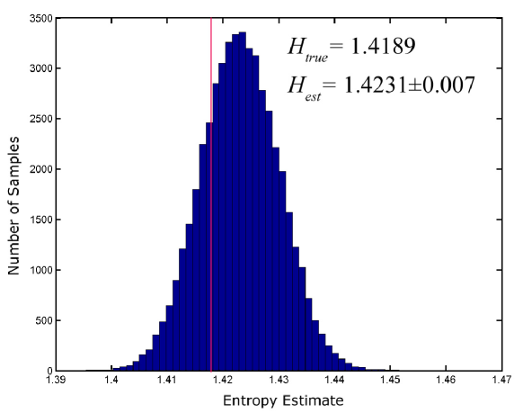
Figure 3: This figure shows the histogram of the entropy samples computed from the bin probabilities drawn from a Dirichlet distribution defined by the data. The true entropy falls within one standard deviation of our estimate.

Say that you have a variable that you know is Gaussian distributed with zero mean and unit variance, $\mathcal{N}(0,1)$. If you want to obtain an instance of this variable that is in accordance with its known Gaussian probability density, you merely need to sample a point from a Gaussian distribution with zero mean and unit variance. It is easy to obtain many such instances by generating many samples, and it is not surprising to find that the mean and variance of those instances is consistent with the density from which they were sampled.

We take the same approach here. Given the number of bins $M$ in the probability density model, the posterior probability (4) of the bin heights has the form of a Dirichlet distribution. One can sample the bin heights from the Dirichlet distribution by sampling each bin height from a gamma distribution with common scale and shape parameters and renormalizing the resulting set to unit probability [8, p. 482]. Every set of bin height samples that is drawn, constitutes a probability density model that could very well describe the given data. By taking something on the order of $50,000$ samples, we have a set of $50,000$ probability density models each of which are probable descriptions of the data. The fact that we get many different, albeit similar, density models is a result of the fact that we are uncertain as to which model is correct. Without an infinite amount of data, we will always be uncertain—the question is: how uncertain? By simply computing the mean and variance of the bin heights from this set of samples, we can confirm that it approaches the theoretical mean (6), and likewise with the height variance (7). This sample variance, or its square root—the standard deviation, of the bin heights quantifies our uncertainty about the probability density.

For each sampled probability density model, we can compute the entropy. This will be given by (10) for a one-dimensional density function, by (11) for a two-dimensional density function, and so on for higher dimensions. The result is a list of $50,000$ or so entropies, from which we can readily compute the mean and standard deviation thus providing us with an entropy estimate and an associated standard deviation quantifying our uncertainty.

In one experiment, $10,000$ data points were sampled from a Gaussian distribution with zero mean and unit variance. The optimal number of bins was found to be $M=24$. The number of counts per bin for each of the $24$ bins was used to sample $50,000$ probability density models from a Dirichlet distribution. From each of these samples, the entropy was computed. Figure 3 shows a histogram of the $50,000$ entropy samples. The mean entropy was found to be $H_{est}=1.4231\pm 0.007$. The true entropy, which is $H_{true}=1.1489$, is within one standard deviation of our estimate. This indicates that $H_{est}$ is a reasonable estimate of the entropy that simultaneously quantifies our uncertainty as to its precise value.

The mutual information and transfer entropy are computed similarly, with the understanding that to compute the mutual information, one works with two-dimensional density functions, and for the transfer entropy one works with three-dimensional densities. Despite the increase in dimensionality, the sampling procedure works exactly as described above for the one-dimensional case.

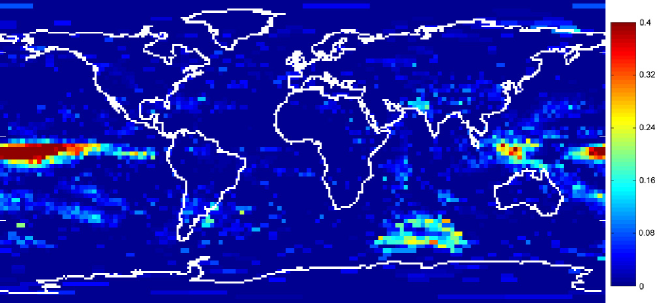
Figure 4: This figure shows a preliminary mutual information map, which quantifies the relationship between the Cold Tongue Index, which is indicative of the equatorial Pacific sea surface temperatures, and the Percent Cloud Cover across the globe.

5 Application to Climate Variables

To demonstrated that the mutual information can identify relationships between climate variables, we performed several preliminary explorations. In one of our explorations, we considered the percent cloud cover (computed as a monthly average) as one subsystem $X$. These data were obtained from the International Satellite Cloud Climatology Project (ISCCP) climate summary product C2 [13, 14], and consisted of monthly averages of percent cloud cover resulting in a time-series of 198 months of 6596 equal-area pixels each with side length of 280 km. It is best to think of the percent cloud cover at each pixel as an independent subsystem, say $X_{1},X_{2},\ldots,X_{6596}$. The other subsystem $Y$ was chosen to be the Cold Tongue Index (CTI), which describes the sea surface temperature anomalies in the eastern equatorial Pacific Ocean (6N-6S, 180-90W)[15]. These anomalies are known to be indicative of the El Niño Southern Oscillation (ENSO)[16, 17]. Thus the second subsystem $Y$ consists of the set of 198 monthly values of CTI, and corresponds in time to the cloud cover subsystems.

The mutual information was computed between $X_{1}$ and $Y$, and $X_{2}$ and $Y$, and so on by using (12). This enables us to generate a global map of 6596 mutual information calculations (Figure 4), which indicates the relationship between the Cold Tongue Index (CTI) and percent cloud cover across the globe. Note that the cloud cover affected by the sea surface temperature (SST) variations lies mainly in the equatorial Pacific, along with an isolated area in Indonesia. The highlighted areas in the Indian longitudes are known artifacts of satellite coverage.

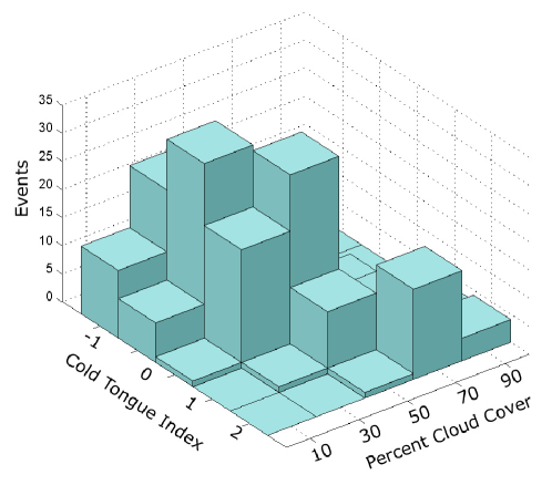
Figure 5: This figure shows the optimal histogram (error bars omitted) of the joint data formed by combining the Cold Tongue Index time series with the Percent Cloud Cover time series at the location where the mutual information was found to be maximal.

Pixel $3231$, which lies in the equatorial Pacific (1.25N 191.25W), was found to have the greatest mutual information. Thus cloud cover at this point is maximally relevant to the CTI and vice versa. By taking the time series representing the percent cloud cover at this position, we can combine this with the CTI time series to construct an optimal two-dimensional density model (Figure 5). This density function is not factorable into the product of two independent one-dimensional density functions. This indicates that the mutual information is non-zero (as we had previously determined), and that the two quantities are related in the sense that one variable provides information about the other.

We are currently working to sample these density functions from their corresponding Dirichlet distributions to obtain more accurate estimates of these information-theoretic quantities along with error bars indicating the uncertainty in our estimates. The end result will be a set of software tools that will allow researchers to rapidly and accurately estimate information-theoretic measures to identify, qualify and quantify causal interactions among climate variables from large climate data sets.

References

- [1] E. N. Lorenz, “Deterministic non-periodic flows,” J. Atmos. Sci., Vol. 20, pp. 130-141, 1963.
- [2] C. F. Shannon, W. Weaver, The Mathematical Theory of Communication, Univ. of Illinois Press, 1949.
- [3] T. M. Cover, J. A. Thomas, Elements of Information Theory, John Wiley & Sons, Inc., 1991.
- [4] C. W. J. Granger, “Investigating causal relations by econometric models and cross-spectral methods,” Economentrica, Vol. 37, No. 3, pp. 424-438, July 1969.
- [5] K. H. Knuth, “Measuring questions: Relevance and its relation to entropy,” in: R. Fischer, V. Dose, R. Preuss, U. v. Toussaint (eds.), Bayesian Inference and Maximum Entropy Methods in Science and Engineering, Garching, Germany 2004, AIP Conf. Proc. 735, American Institute of Physics, Melville NY, pp. 517-524, 2004.
- [6] K. H. Knuth, “Lattice duality: The origin of probability and entropy”, in press Neurocomputing, 2005.
- [7] D. S. Sivia, Data Analysis. A Bayesian Tutorial, Clarendon Press, 1996.
- [8] A. Gelman, J. B. Carlin, H. S. Stern, D. B. Rubin, Bayesian Data Analysis, Chapman & Hall/CRC, 1995.
- [9] K. H. Knuth, “Optimal data-based binning for histograms”, in submission, 2005.
- [10] M. Abramowitz, I. A. Stegun, Handbook of Mathematical Functions, Dover Publications Inc., 1972.
- [11] T. Schreiber, “Measuring information transfer,” Phys Rev Lett Vol. 85, pp. 461-464, 2000.
- [12] A. J. Bell, “The co-information lattice,” in: T.-W. Lee, J.-F. Cardoso, E. Oja and S. Amari (eds.), Proc. 4th Int. Symp. on Independent Component Analysis and Blind Source Separation (ICA2003), pp. 921-926, 2003.
- [13] R. A. Schiffer, W. B. Rossow, “The International Satellite Cloud Climatology Project (ISCCP): The first project of the world climate research programme,” Bull. Amer. Meteor. Soc., Vol. 64, pp. 779-784, 1983.
- [14] W. B. Rossow, R. A. Schiffer, “Advances in understanding clouds from ISCCP,” Bull. Amer. Meteor. Soc., Vol. 80, pp. 2261-2288, 1999.
- [15] C. Deser, J. M. Wallace, “Large-scale atmospheric circulation features of warm and cold episodes in the tropical Pacific,” J. Climate, Vol. 3, pp. 1254-1281, 1990.
- [16] C. Deser, J. M. Wallace, “El Niño events and their relation to the Southern Oscillation: 1925-1986,” J. Geophys. Res., Vol. 92, pp. 14189-14196.
- [17] T. P. Mitchell, J. M. Wallace, “ENSO seasonality: 1950-78 versus 1979-92,” J. Climate, Vol. 9, pp. 3149-3161, 1996.